International Journal of Engineering
J o u r n a l H o m e p a g e : w w w . i j e . i r
Optimal Design of the Cross-docking in Distribution Networks: Heuristic Solution
Approach
S. M. Mousavi* a,b , R. Tavakkoli-Moghaddam a, A. Siadat b
a School of Industrial Engineering, College of Engineering, University of Tehran, Tehran, Iran b LCFC, Arts et Métier Paris Tech, Metz, France
P A P E R I N F O
Paper history: Received 30 March 2013
Received in revised form 17 May 2013 Accepted 22 August 2013
Keywords:
Logistics Management
Cross-Docking Distribution Networks Mixed-Integer Programming (MIP) Model Heuristics
Simulated Annealing
A B S T R A C T
Cross-docking plays an importation role in distribution networks. In the recent years, a cross-docking design network problem is addressed as a new research area in logistics management. This paper presents a new mathematical model for the location of cross-docking facilities and vehicle routing scheduling problems in the distribution networks. For this purpose, a two-phase mixed-integer programming (MIP) is formulated. Then, a new heuristic-based simulated annealing (SA) is developed for solving the proposed MIP model. Finally, the presented heuristic algorithm is subsequently tested on a number of small and large-scale instances. The computational results for different-sized instances illustrate that the proposed algorithm performs effectively in a reasonable time.
doi: 10.5829/idosi.ije.2014.27.04a.04
1. INTRODUCTION1
A cross-docking distribution network can be defined as the delivery of enhanced customer and economic value through synchronized management of the flow of physical products and related information from suppliers to customers in the limited time available (e.g., two days). A network of autonomous business cross-docking facilities is considered, in which the arriving goods are transferred by vehicles (e.g., trucks) and are delivered to the retailers or customers as rapidly as possible. The performance of any node in the distribution network depends on the performance of other nodes, and their ability to coordinate activities within the network. Thus, designing this distribution network with the cross-docking can be considered as an important issue in logistics management [1-4].
To design the cross-docking distribution network, in this paper location of cross-docking facilities and vehicle routing scheduling are considered. This problem is known as NP-hard problem [1, 5]; by increasing sizes of this problem, there is a need to utilize heuristic and
*Corresponding Author Email:[email protected] (S. M. Mousavi)
meta-heuristic algorithms as effective solving approaches. The exact algorithms need exponential CPU time by considering the size of the problems.
In the related literature, there exist some studies focusing on distribution planning problems with the cross-docking. For instance, Jayaraman and Ross [1] presented a practical approach for solving a multiple product, multi-echelon problem for distribution network design by the simulated annealing (SA) algorithm. Li et al. [6] addressed a cross-docking facility operation in order to eliminate or minimize storage and order picking activity in the cross-docking using just-in-time (JIT) scheduling. Lee et al. [5] presented an integration model of cross-docking facilities with vehicle routing scheduling for the distribution network design problem. Ross and Jayaraman [7] addressed an evaluation of heuristics for the location of cross-docking facilities in the supply chain. Musa et al. [8] considered the transportation problem of a cross-docking network, in which loads were transferred from suppliers to retailers through cross-docking facilities. Belle et al. [9] provided a review of the existing literature about cross-docking. The papers were classified according to the problem type ranging from more strategic or tactical to more operational problems. Liao [10] considered the
simultaneous dock assignment and sequencing of inbound trucks for a multi-door cross-docking operation with the objective to minimize total weighted tardiness, under a fixed outbound truck departure schedule.
Regarding the recent developments of the cross-docking systems, Boysen and Fliedner [11] proposed a classification of truck scheduling problems, and then future research needs were identified. Acar et al. [12] presented a mixed integer quadratic model with the objective of generating trailer-to-door assignments which equally distribute idle times at doors to accommodate operational level uncertainty by considering truck arrival times. Then, a heuristic was introduced for the door assignment. Shakeri et al. [13] considered truck scheduling in a resource-constrained cross-docking, and the sequence of incoming and outgoing trucks at the dock doors of the cross-docking terminal by regarding the availability of cross-dock resources. Then, an algorithmic approach was extended which was capable of establishing solution feasibility for the problem. Hu et al. [14] formulated the optimal route selection problems in the fashion supply chain from the suppliers to the cross-docking center and from the cross-docking center to the customers as the respective vehicle routing problem. Konur and Golias [15] addressed the cross-dock operator’s problem and proposed a cost-stable scheduling strategy while minimizing the average of total service costs. Also, a bi-objective bi-level optimization problem was formulated and a genetic algorithm was developed.
This paper introduces a new two-phase mixed-integer programming (MIP) model for designing cross-docking distribution networks. Then, a new heuristic-based SA is presented that characterizes a special solution representation scheme for the location of cross-docking and routing scheduling in the distribution networks. The computational results indicate that the proposed solving approach performs well on small and large-scale problems within a reasonable amount of time.
The structure of this paper is organized in six sections. In the next section, the problem definition is defined, and then a new two-phase MIP model is proposed in Section 3. The problem-solving approach is described in Section 4. Computational results are discussed in Section 5. Finally, conclusions are provided in Section 6.
2. PROBLEM DEFINITION
Cross-docking is a distribution network to decrease inventory while satisfying customers’ requirements. Through streamlining the flow between the suppliers and manufacturers, this distribution can help to reduce or eliminate inventory storage.
Figure 1. Concept of the proposed cross-docking distribution network
The cross-docking copes with the movement of goods directly from the receiving dock to the shipping dock, in which the goods are stored in cross-docking facilities for a short time or directly transformed to the customers [2]. In fact, the inventory holding function of a traditional warehouse can be eliminated by the cross-docking while still goods need to be classified and loaded to the delivery vehicles through a consolidation process [2, 5]. The concept of proposed distribution network with the cross-docking is illustrated in Figure 1, in which two main nodes are simultaneous arrival and consolidation.
The location of cross-docking facilities and vehicle routing scheduling problems can be stated as follows: given a set of retailers with known demand and a set of potential cross-docking facilities, the location of the cross-docking facilities is determined in the first phase. Then, the vehicle routing scheduling from the cross-docking facilities is obtained in the pickup and delivery processes to minimize the sum of the costs associated with the location of cross-docking facilities and distribution from suppliers / to the retailers. In the first phase, three types of costs are minimized. The first type of costs is fixed costs associated with operating open cross-docking facilities. The second type is costs to transport units of the product from suppliers to cross-docking facilities and from cross-cross-docking facilities to retailers. The third type is the cost of holding inventories at cross-docking facilities. In addition, in the second phase distribution costs are considered associated with the routing of vehicles, containing operational costs of vehicles and transportation costs.
designed so that the demand of each customer can be satisfied. Each customer is served by only one vehicle. The total demand on each route is less than or equal to the capacity of the vehicle assigned to that route. Each route starts and ends at the same cross-docking facility. Also, the total quantity of pickup should equal the quantity to be delivered. It is assumed that all vehicles are located in the multiple cross-docking facilities, and split pickups and deliveries are not allowed.
3. PROPOSED MODEL FORMULATION
The following notations are used in formulation of the proposed MIP model for the cross-docking location problem in the first phase, and vehicle routing scheduling problem with multiple cross-docking facilities in the second phase.
3. 1. Sets and Input Parameters
P: Set of suppliers (i =1, 2, ..., n)
D: Set of retailers (i¢ =1, 2, ..., m)
O: Set of cross-docking facilities (o= 1, 2, …, c)
T: Set of time (t = tmin , …, tmax)
Ami: Amount of product in pickup node i
i
Am¢: Amount of product in delivery node i¢
Disti,o: Distance of pickup node i from cross-docking facility
o
o i
Dist¢, :Distance of delivery node i¢ from cross-docking
facility o
Capo : Capacity of cross-docking facility o
HCo : Holding cost per unit productin a unit of time at
cross-docking facility o
Tmin , Tmax : Minimum and maximum of time horizon
Fo: Fixed cost to open cross-docking facility o
R: Maximum number of cross-docking facilities to be opened
K: Number of available vehicles in the pickup process
K¢: Number of available vehicles in the delivery process
i
d¢: Unloaded amount of product in node i¢in the delivery process
Q: Maximum capacity of each vehicle
cij: Transportation cost from node i to node j in the pickup process
j i
c¢¢: Transportation cost from node i¢ to nodej¢in the delivery process
ck: Operational cost of vehicle k
k
c ¢:Operational cost of vehicle k¢
dij: Distance from node i to node j in the pickup process
j i
d¢¢: Distance from node i to node j¢ in the delivery process
k i
t : Length of a visit for vehicle k in node i in the pickup process
k i
t¢¢: Length of a visit for vehicle k¢ in node i¢ in the delivery process
etij: Time for the vehicle to move from node i to node j in the pickup process
j i
et¢¢: Time for the vehicle to move from nodei¢ to nodej¢ in the delivery process
3. 2. Decision Variables i
t o
X, : 1 if productinpickup i goes to cross-docking facility o
at time t, and 0 otherwise i
t o
X¢, : 1 if product in delivery i¢is bound for cross-docking
facility o at time t, and 0 otherwise
So,t: Amount of productat cross-docking facility o at time t
xo: 1 if cross-docking facility o is open, and 0 otherwise. k
ij
X :1 if vehicle k transports product from node i to node j in the pickup process, and 0 otherwise
k j i
X¢¢¢:1 if vehicle k transports product from i¢ to nodej¢in the
delivery process, and 0 otherwise
ij
y : Transported amount of product from node i to node j in the pickup process
j i
Z¢¢: Transported amount of product from nodei¢ to node j¢ delivery process
k i
DT : Departure time of vehicle k from node i in the pickup process
k i
DT¢¢: Departure time of vehicle k¢ from node i¢ in the
delivery process
k j
DT : Departure time of vehicle k from node j in the pickup
process
k j
DT¢¢: Departure time of vehicle k¢ from node j¢ in the
delivery process
k j
k j
AT¢¢: Arrival time of vehicle k¢ from node j¢ in delivery
process
k o
AT : Arrival time of vehicle k at cross-docking facility o in the pickup process
k o
AT¢¢: Arrival time of vehicle k¢ at cross-docking facility o¢
delivery process
3. 3. Cross-docking Facilities Location (Phase 1) The location problem of cross-docking facilities can be formulated as below:
o i n i c o T T
t io
i t o o i m i c o T T
t i o
i t o c o T T
t o ot
c
o o o
C Dist X C Dist X S HC x F MinZ , , , , , , , max min max min max min
å å å
å å å
å å
å
= = = ¢ = ¢ = = ¢ ¢ = = = + + + = 1 1 1 1 1 1 1 (1) s.t. i X c o Ts T t i t od = "¢
å å
=-= ¢ min , 0 1 1 (2) i X c o TE TS t i t o d d ¢ " £
å å
= =¢ , 1 1 (3) i X c o T TE t i t o d ¢ " =
å å
= = +¢ max
, 0
1 1 (4)
i X c o Ts T t i t o
p = "
å å
=
-= min , 0 1 1 (5) i X c o TE TS t i t o p p " =
å å
=1 = , 1 (6)i X c o T TE t i t o p " =
å å
= = +max
, 0
1 1 (7)
max min , , T t T Am X Am X C o m i i i t o C o n i i i t o £ £ "
³
å å
å å
=1 =1 =1 ¢=1 ¢ ¢ (8)o
so,Tmin-1=0 " (9)
max min , , , , and
T t T o Am X Am X s s n i i i t o m i i i t o t o t o £ £ " +
-=
å
å
= =
¢ ¢
¢
-1 1 1 (10)
max min
, cap o and T t T
Sot£ o " £ £ (11)
max min
, x i,o and T t T
Xoi t£ o " £ £ (12)
max min
, x i,o and T t T
Xoi¢t£ o "¢ £ £ (13)
R x
c
o o£
å
=1 (14){ }
0,1 ,, , , oi¢t oÎ i
t
o X x
X (15)
0
³
t o
S, (16)
Objective function (1) minimizes the total costs including costs of holding inventories at cross-docking facilities and costs of transportation, namely costs of transportation from suppliers to cross-docking facilities and then from cross-docking facilities to retailers. Constraints (2), (3) and (4) ensure that each delivery, if necessary, is fulfilled within its specified time window and beyond that range it takes the value of zero. Constraints (5), (6) and (7) guarantee the time window restriction for pickups. Constraint (8) ensures the sufficient inventory of product to meet all demands. Constraint (9) sets a zero initial inventory for product at each cross-docking facility. Changes in the inventory level of each cross-docking facility at each time are indicated by constraint (10). Constraint (11) describes the potential capacity of cross-docking facilities. Constraints (12) and (13) ensure that transporting product from suppliers to cross-docking facility and from cross-docking facility to retailers in the pickup and delivery processes can be performed only when the corresponding cross-docking facility is open. Constraint (14) limits the number of cross-docking facilities that can be located. Constraints (15) and (16) define decision variables of the model.
3. 4. Vehicle Route Scheduling (Phase 2): The vehicle route scheduling problem with multiple cross-docking facilities can be formulated by:
(
)
( )(
)
[
]
( )(
)
( )(
)
[
]
( )å
å å
å å
å
å
å å
å å
å
Î ¢ ¢= ¢ = ¢ ¢ ¢ ¢ ¢ ¢ ¢ =
¢ ¢Î
¢ =
¢ ¢¢ ¢¢ ¢
Î = =
= Î =
¢ ¢ ¢ ¢ + + + + + = O D i m j K k k k j i j i m
i j D O
K k k j i j i O P i n j K k k ij k ij ij n
i j P O
K k k ij ij ij j i j i x c d c x d c x c d c x d c Z Min U U U U 1 1 1 1 1 1 1 1 2 (17) s.t.
(P O) x j
i
K k
k
ij= "
å
Î Uå
=1 1 (18)(P O) x i
j
K k
k
ij= "
å
Î Uå
=1 1 (19)(D O) x j
i
K k
k j
i = "¢
å
¢Îå
¢ = ¢ ¢ ¢ ¢ 1 1 U (20)
(D O) x i
j
K k
k j
i = "¢
å
¢Îå
¢ =
¢ 1 ¢¢¢ 1
U (21)
(P O) x j O
i
K k
k
ij³ "Î
(D O) x j O i K k k j
i ³ "¢Î
å
¢Îå
¢ = ¢ ¢ ¢ ¢ 1 1 U (23)
( )x j (P O)x kr (P O) k rj O P i k
ir U U
U =
å
" Îå
Î Î , (24)( )x j (D O)x k r (D O) k j r O D i k r
i U U
U =
å
"¢ Îå
¢Î¢ ¢ ¢ Î ¢ ¢ ¢
¢ , (25)
( )
(P O) x k
i j P O
k
ij£ "
å
Î Uå
Î U 1 (26)( )
(D O) x k
i j D O
k j
i £ " ¢
å
¢Îå
¢Î¢ ¢
¢ 1
U U (27)
( )
(P O) x K
i j P O
K k
k ij£
å
Î Uå
Î Uå
=1 (28)( )
(D O) x K
i j D O
K k
k j
i £ ¢
å
¢Îå
¢Îå
¢ = ¢ ¢ ¢ ¢
U U 1 (29)
(P O)
j i Q
yij£ ", Î U (30)
(D O)
j i Q
zi¢j¢£ "¢, ¢Î U (31)
å
å
= = ¢= ¢m
i i
n
i 1pi 1d (32)
r j P i if p y
yjr= ij- j Î ,", (33)
r j O i if p y
yjr= ij-
å
in=1 j Î ,", (34)r j D i if d z
zi¢j¢= i¢r¢+ j¢ ¢Î ,"¢, ¢ (35)
r j O i if d z z m i i r j j
i¢¢= ¢¢+
å
¢= ¢ ¢Î ,"¢, ¢1 (36)
(n ) i j
x n u u K k k ij j
i- +
å
=1 £ -1 ", (37)(m ) i j
x m u u K k k j i j
i- +
å
£ - "¢ ¢¢ = ¢ ¢ ¢ ¢ ¢
¢ 1 ,
1 (38)
(
et DT t)
x ki jDTjT³ ij+ ik+ki ijk " ,, (39)
(
et DT t)
x k i jDTTj¢¢³ i¢j¢+ i¢k¢+ik¢¢ ik¢j¢¢ " ¢,¢, ¢ (40)
(
DT et)
x ki j OATkj³ ik+ ij ijk " ,,"Î (41)
(
DT et)
x k i j OATkj¢¢³ i¢k¢+ i¢j¢ ik¢j¢¢ " ¢,¢,"¢Î (42)
o o k k AT
ATok= ok¢¢¢ " ¹ ¢¢," ¹ ¢ (43)
o o k k AT
ATok¢= ok¢¢¢¢ " ¢¹ ¢¢¢," ¹ ¢ (44)
i n
ui£ " (45)
j n
uj£ " (46)
i m
ui¢£ "¢ (47)
j m
uj¢£ "¢ (48)
{ }
i ji jx
xijk, ik¢j¢¢Î 0,1 " , , ¢, ¢ (49)
k k o o j i j i u u u u AT AT DT DT DT DT z y j i j i k o k o k j k j k i k i j i ij ¢ ¢ ¢ ¢ " ³ ¢ ¢ ¢ ¢ ¢ ¢ ¢ ¢ ¢ ¢ , , , , , , , , , , , , , , , , , , 0 (50)
The objective function (17) minimizes total
transportation costs associated with moving product in the pickup and deliver processes as well as operational cost of each vehicle in these processes separately. Constraints (18) and (19) show that one vehicle has to arrive at and leave one node in the pickup process. Constraints (20) and (21) show that one vehicle has to arrive at and leave one node in the delivery process. Constraints (22) and (23) specify that every supplier or retailer belongs to one and only one route, but cross-docking facilities may belong to more than one route. Constraints (24) and (25) express the consecutive movement of vehicles. Whether or not a vehicle arrives at and leaves a cross-docking facility in the pickup and delivery processes is shown in constraints (26) and (27). Constraints (28) and (29) ensure that the numbers of vehicles that arrive or leave a cross-docking facility in the pickup or delivery processes must be less than the number of available vehicles. Constraints (30) and (31) express that the quantity of loaded product in a vehicle cannot exceed the maximum capacity of the vehicle. The flow conservation for product is manifested in constraint (32). The quantity of products between nodes in the pickup and delivery processes is shown in constraints (33) – (36). Constraints (37) and (38) ensure that every retailer is on a route connected to the set of cross-docking facilities. Constraints (39) and (40) express that the departure time of a vehicle from a node is determined by the sum of the arrival time at a node, the length of a visit, and time to move in the pickup and delivery processes. The arrival time at a cross-docking facility is represented in constraints (41) and (42) for the pickup and delivery processes. The constraints for simultaneous arrival to a cross-docking facility are given in Equations (43) and (44). Constraints (45) – (50) enforce the integrality restrictions on the decision variables.
4. PROPOSED HEURISTIC
The proposed heuristic for designing cross-docking distribution networks is based on the SA algorithm. The SA can be regarded as a local search-based algorithm, and can be able to escape from being trapped into a local optimum by accepting with small probability worse solutions during its iterations. The concept of the algorithm is based on the annealing process applied to the metallurgical industry [1]. This algorithm has been successfully employed to numerous complicated combinatorial optimization problems as well as a wide range of real-world problems [e.g., 1, 7].
The search for least-cost solutions is guided by a control parameter, known as temperature (T), and this temperature determines the acceptance of inferior solutions. Proposed algorithm begins with a randomly generated initial configuration which specifies the cross-docking facilities to be opened, the suppliers and retailers assigned to the cross-docking facilities. The total cost is computed by the objective function of the proposed model.
Step 1: Initialization Initial and final values of the control parameter temperature are considered, known as
T0 and Tf respectively. An initial cross-docking facility solution is randomly obtained by assigning supply of suppliers and demand flows of retailers between pickup, docking facilities and delivery nodes in the cross-docking distribution network. This results in an initial feasible solution by producing product flows. The objective function value of this solution can be regarded as the objective function value for the best configuration found best solution (BS), current configuration C(Φ), and the newest configuration C(Φ¢). All counters are set to 1.
Step 2: Check Feasibilities The algorithm now assesses product flow assignments for cross-docking facilities to make sure that the capacity of each cross-docking facility, investment opening cost and numbers of potential cross-docking facilities are satisfied. Furthermore, we check that quantity of product and demand of customer should be satisfied. If the configuration is not feasible, we return to step 1.
Step 3: Provide a Feasible Neighboring Solution Once the network design problem has been initialized, an objective function value is calculated, and feasibility ensured, the current feasible cross-docking system configuration is then updated by choosing a supplier and reassigning the amount of product between a cross-docking facility and supplier. On the other hand, this procedure can be utilized for retailers. They are accomplished by randomly choosing a supplier and a customer to perturb. Its flow is randomly allocated to another combination of pickup / cross-docking facility / delivery nodes. All feasibilities are investigated once again. Finally, the objective function value of the neighboring solution C(Φ¢)is determined.
Step 4: Assess Current Solution with Neighboring Solution If the objective function value of the neighboring solution is greater than that of the current solution (C(Φ¢)>C(Φ)), process to Step 5. Otherwise, if the objective functions value of the newest configuration improves over the current solution (
) ( )
(Φ C Φ
C ¢ < ), the neighboring solution can be regarded as the current solution. Then, this solution is compared to BS (i.e., the best solution obtained thus far). If the objective function value of the newest configuration is less than that of the best one found so far (C(Φ¢)<BS), then replace the best solution with that of the neighboring solution process to step 6.
Step 5: Investigate Metropolis Condition The difference (Dcost) between the neighboring solution and
the current solution is calculated, as
)) ( ) ( cost
(D =CΦ¢ >C Φ . Then, the Metropolis criterion is
applied to obtain the probability at which the relatively inferior neighboring solution can be accepted, P(A). This probability is calculated by [1]:
) cost/ exp( )
(A Ti
P = D (51)
where Ti is the current temperature. A random number is then generated from the interval (0,1). If this random number is less than P(A), then the neighboring solution replaces the current solution. Proceed to Step 6.
Step 6: Increase counters. Memory and status variables are updated. The counters are incremented by one. If the iteration counter value is less than or equal to the maximum iterations for the temperature level, then return to Step 3. Otherwise go to Step 7.
Step 7: Adjust Temperature Temperature is adjusted in iteration i by the cooling rate. Mathematically, we have:
) ln(
) ln(
N T T
i
f o
i T T
-= 0 (52)
If the new value of Ti is greater than or equal to the stopping value (Tf), then reset iteration counters to one and return to Step 3. Otherwise, stop.
4. 2. Proposed Heuristic for Vehicle Routing Scheduling (Phase 2) This sub-section explains the algorithmic steps of the heuristic-based SA for the routing scheduling problem, providing insight into the progress of the search.
route, a vehicle starts from the cross-docking facility, which is illustrated as 0, travels to suppliers 2, 3 and finally supplier 5. After that, the vehicle returns back to the cross-docking facility. In the second route, the vehicle starts with supplier 6 and then supplier 1. Similarly, the vehicle travels back to the cross-docking facility after serving the suppliers. In the third route, the vehicle starts with supplier 4 and then supplier 7. Similarly, the vehicle travels back to the cross-docking facility after serving the suppliers. In the same way, this procedure will be utilized for delivery processes.
It is pointed out that each solution contains O links if there are O cross-docking facilities in the vehicle routing scheduling problem. For this problem in the step of initialization, there are three sub-steps to generate a feasible initial solution. The first sub-step is to assign suppliers / retailers to each of the O links, that is, the grouping problem. There are a number of cross-docking facilities, suppliers and retailers, and each supplier / retailer should be allocated to one cross-docking facility or link. Because the objective function is to minimize the total distribution costs, suppliers and retailers are assigned to the cross-docking facility which is minimum distribution cost. The second sub-step is to assign suppliers / retailers in the same link to several routes by using the saving method in [16]. The method constructs a saving matrix for every two suppliers / retailers in the same link. Then, the suppliers / retailers with large saving value are grouped in the same route while not violating the vehicle capacity constraint and arrival time constraint. The third sub-step is to solve the scheduling problem by the NNH in [17]. The principle of the NNH is to randomly begin with the first supplier and retailer. Then, the next customer / retailer is chosen as minimum cost to the previous one from those unselected suppliers/retailers to build the pickup and delivery sequence until all suppliers and retailers are chosen.
Step 2: Improvement This procedure is based on the SA to improve upon the best solution obtained at any step of the algorithm. The algorithm is described as follows:
For i = 1–n do For i¢= 1–m do
(a) Initialize max-iterations, initial temperature.
Set count = 1, T0= temp-start.
(b) Let the best solution obtaining in the initialization step be called the current solution, xc.
Compute the objective function for current solution, OBF(xc).
Randomly generate a neighbouring solution using either the interchange
neighbourhood; forward insertion neighbourhood or backward insertion neighbourhood. Let neighbouring solution called the adjacent solution, xa. Compute objective function for adjacent solution, OBF(xa )
(c) If OBF(xa) <OBF(xc)
Then set xc = xa ; Else
SetD=OBF(xa) -OBF(xc); Set T = temp-start/log(1+count); With probability e-DTset xc = xa.
Increment count by 1.
(d) If count < max-iteration, go to Step (b).
The output of the current solution is applied as the final solution. The annealing schedule used in Step (c) of the above algorithm is based on [18]. The interchange neighborhood, by far the most popular scheme, is simple: swap two randomly chosen supplier / retailers in the pickup and delivery sequence. In forward insertion neighborhood a supplier / retailer is relocated further forward in the sequence, and in backward insertion neighborhood a supplier / retailer is relocated further backward in the sequence. Figures 2 and 3 show the solution representations of an example and visual illustrations by the proposed heuristic-based SA algorithm for the second phase of the MIP model.
5. COMPUTATIONAL RESULTS
solutions for the first and second phases are 3.22% and 3.70% indicating the efficiency of the proposed heuristic-based SA algorithm in the distribution network. Moreover, increasing the size of the two-phase cross-docking distribution network problem increases the solution time of GAMS exponentially while it does not have significant impacts on the solution time of the proposed algorithm.
Figure 2. Example of solution representations
Figure 3. Visual illustrations of the example solution
TABLE 1. Sizes of small test problems
Problem no. No. of suppliers (n) No. of potential cross-docking facilities (c) No. of retailers (m)
1 3 2 4
2 4 3 5
3 5 3 6
4 7 4 8
5 8 5 9
6 9 6 10
7 10 7 11
8 11 8 12
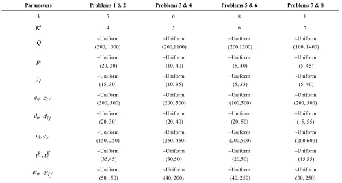
TABLE 2. Sources of random generations for the first phase of proposed MIP model
Parameters Problems 1 & 2 Problems 3 & 4 Problems 5 & 6 Problems 7 & 8
HCo
~Uniform (100, 200)
~Uniform (120, 220)
~Uniform (180, 280)
~Uniform (180, 300)
Disti,o, Disti¢,o ~Uniform
(20, 40)
~Uniform (25, 45)
~Uniform (30, 50)
~Uniform (20, 45)
TC ~Uniform
(5000, 6000)
~Uniform (9500, 12500)
~Uniform (15000, 18000)
~Uniform (12500, 18000)
R 2 3 4 6
Capo ~Uniform (200, 500)
~Uniform (350, 700)
~Uniform (500, 800)
~Uniform (400, 600)
Fo
~Uniform (2000, 5000)
~Uniform (2500, 5500)
~Uniform (3000, 6000)
TABLE 3. Sources of random generations for the second phase of the proposed MIP model
Parameters Problems 1 & 2 Problems 3 & 4 Problems 5 & 6 Problems 7 & 8
k 5 6 8 8
K¢ 4 5 6 7
Q ~Uniform
(200, 1000)
~Uniform (200,1100)
~Uniform (200,1200)
~Uniform (100, 1400)
pi
~Uniform (20, 30)
~Uniform (10, 40)
~Uniform (5, 40)
~Uniform (5, 45)
i
d¢ ~Uniform (15, 30) ~Uniform (10, 35) ~Uniform (5, 35) ~Uniform (5, 40)
cij, ci¢j¢ ~Uniform
(300, 500)
~Uniform (200, 500)
~Uniform (100,500)
~Uniform (200, 500)
dij, di¢j¢ ~Uniform
(20, 30)
~Uniform (20, 40)
~Uniform (20, 50)
~Uniform (15, 55)
ck,ck¢ ~Uniform
(150, 250)
~Uniform (250, 450)
~Uniform (200,500)
~Uniform (200,600)
k i
t ,tik¢¢ ~Uniform
(35,45)
~Uniform (30,50)
~Uniform (20,50)
~Uniform (15,55)
etij, eti¢j¢ ~Uniform (50,150)
~Uniform (40, 200)
~Uniform (40, 250)
~Uniform (30, 250)
TABLE 4. Results in small-sized test problems for the first phase
Proposed heuristic-based SA (400 iterations) GAMS
No. of test problems
Gap (%) Time (s)
Best solution Time (s)
Best solution
1.36 24.6
5951.4 31.6
5871.6 1
2.75 28
11048.8 55.2
10753.4 2
2.80 30
11858 83.2
11534.6 3
2.41 30.5
25390.4 104.5
24794 4
6.04 34
34305.6 111.7
32352.6 5
3.34 36.2
38207.4 149
36974 6
3.51 36.5
50831.2 230.5
49106.4 7
3.60 41
57909 248
55897 8
3.22
32.6 29437.7
126.7 28410.5
Average
TABLE 5. Results in small-sized test problems for the second phase
Proposed heuristic-based SA (400 iterations) GAMS
No. of test problems
Gap (%) Time (s)
Best solution Time (s)
Best solution
1.22 38.5
95100.6 41
92848 1
4.69 42
178544.8 138.2
170552.2 2
1.50 45
254265.2 152
250507.6 3
2.22 44
317483.6 156
310597 4
3.60 47
373576 198
360578.4 5
7.21 50.5
480480 205.9
448172.2 6
4.39 56.4
504180.6 349.5
482970.6 7
3.60 52
579090 370.6
558970 8
3.70 46.9
282692.5 201.4
271515.4 Average
TABLE 6. Results in large-sized test problems for the first phase Proposed heuristic-based SA (600 iterations) Proposed heuristic-based SA (400 iterations) GAMS No. of retailers No. of
cross-docking facilities No. of
suppliers No. of test
problems Time (s) Best solution Time (s) Best solution Time (s) Best solution 340.5 46998 305.5 47136 -30 10 25 1 493.4 54901 335.6 56966 -35 12 30 2 508.7 50241.6 374.1 51171.2 -40 15 35 3 490.9 62563.2 412.2 63030 -45 18 40 4 452.4 63792 327 66592 -50 20 45 5 589 75032 449.7 75694.4 -55 22 50 6 508 71808 454.3 72683 -60 24 55 7 513.5 80012.3 462 81265 -65 26 55 8 484.9 80374.4 451 82006.2 -74 29 60 9 631 83998 478.8 85798.9 -76 34 65 10 501.2 66972.1 405 68234.3 - - 53 21 46 Average
TABLE 7. Results in large-sized test problems for the second phase
Proposed heuristic-based SA (600 iterations) Proposed heuristic-based SA (400 iterations) GAMS No. of retailers No. of
cross-docking facilities No. of
suppliers No. of test
problems Time (s) Best solution Time (s) Best solution Time (s) Best solution 577.2 552648 381 620386.8 -30 10 25 1 622.6 601915.7 448.4 673271 -35 12 30 2 594.2 576737.5 407.7 677230 -40 15 35 3 654.8 561984.3 474.6 618782.3 -45 18 40 4 611 611115.8 488 715091.7 -50 20 45 5 636.4 655716.5 475.8 738085.5 -55 22 50 6 688 644447 526.3 773760.9 -60 24 55 7 672.9 832180.7 605.8 852403.6 -65 26 55 8 722.9 833414 608 871999.4 -74 29 60 9 731.3 884817 618.5 890100 -76 34 65 10 651.1 675497.7 503.4 743111.1 -53 21 46 Average
For small-sized test problems, the reported gap in Tables 4 and 5 are calculated as below which denotes the gap between the optimal solutions and solutions obtained by the proposed heuristic-based SA algorithm by: . 100 ´ -solution optimal solution optimal heuristic obj obj obj (53)
Figure 4. Convergence rate for the tenth large-sized test problem in the first phase
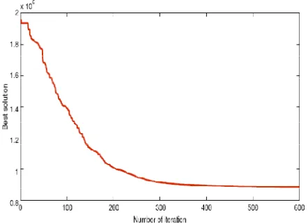
Figure 5. Convergence rate for the tenth large-sized test problem in the second phase
iterations are 503.4 (s) and 651.1 (s), respectively (See Table 7). The best results are provided for 600 iterations in all large-sized test problems. The proposed heuristic run time is acceptable for solving these test problems. For the first phase of the proposed MIP model, the maximum run time in 400 and 600 iterations are 478.8 (s) and 631 (s), respectively, and for the second phase the maximum run time are 618.5 (s) and 731.3 (s) for tenth large-sized test problem. Also, the convergence rates of the proposed heuristic are depicted in Figures 4 and 5 for the tenth test problem.
6. CONCLUSIONS
Logistics managers require making appropriate decisions regarding both qualitative and quantitative aspects to improve the design of the cross-docking
distribution networks. Appropriate decisions must be particularly made concerning the location of cross-docking facilities, the structure of the fleet and the strategies to satisfy customers' requirements with their services. It can be conducted within the framework, in which the location and routing scheduling problems through the cross-docking are studied. This paper
introduced a new two-phase mixed-integer
programming (MIP) model for the location of cross-docking facilities and vehicle routing scheduling in the cross-docking distribution networks. Then, a new heuristic-based simulated annealing (SA) was presented for these problems by considering a special solution representation scheme. The heuristic, hybridized location and routing scheduling decisions, is needed in order to provide high quality solutions with reasonable computational time. To verify the proposed heuristic-based SA, seven small-sized test problems were solved by GAMS software. The computational results obtained by the heuristic were efficient approaching to the optimal solution. The average gap between the proposed heuristic algorithm and GAMS solutions for the first and second phases was equal to 3.22% and 3.70% illustrating the acceptable results, respectively. In addition, the proposed-solving approach was employed to solve the presented MIP model for ten large-scale instances. These solutions demonstrated that the presented MIP model was verified, and the proposed heuristic-based SA provided as an effective problem-solving approach in term of solutions quality and computational time. For the future research, the proposed model can be presented under uncertainty, particularly for the influential parameters that can be provided in fuzzy or stochastic values. It can exert considerable adverse influences on important decisions made by top managers in the cross-docking distribution networks.
7. ACKNOWLEDGMENTS
This work has been partially supported by the Center for International Scientific Studies & Collaboration (CISSC) and the French Embassy in Tehran. The authors are also grateful for the financial support from the Égide Program in France.
8. REFERENCES
1. Jayaraman, V. and Ross, A., "A simulated annealing methodology to distribution network design and management",
European Journal of Operational Research, Vol. 144, No. 3, (2003), 629-645.
3. Mousavi, S. M., Tavakkoli-Moghaddam, R. and Jolai, F., "A possibilistic programming approach for the location problem of multiple cross-docks and vehicle routing scheduling under uncertainty", Engineering Optimization, Vol. 45, No. 10, (2013), 1223-1249.
4. Mousavi, S. M., Tavakkoli-Moghaddam, R., Siadat, A. and Vahdani, B., A hybrid simulated annealing algorithm for location of cross-docking centers in a supply chain, in Hybrid metaheuristics., Springer. (2013), 12-21.
5. Lee, Y. H., Jung, J. W. and Lee, K. M., "Vehicle routing scheduling for cross-docking in the supply chain", Computers & Industrial Engineering, Vol. 51, No. 2, (2006), 247-256. 6. Li, Y., Lim, A. and Rodrigues, B., "Crossdocking—jit
scheduling with time windows", Journal of the Operational Research Society, Vol. 55, No. 12, (2004), 1342-1351. 7. Ross, A. and Jayaraman, V., "An evaluation of new heuristics
for the location of cross-docks distribution centers in supply chain network design", Computers & Industrial Engineering, Vol. 55, No. 1, (2008), 64-79.
8. Musa, R., Arnaout, J.-P. and Jung, H., "Ant colony optimization algorithm to solve for the transportation problem of cross-docking network", Computers & Industrial Engineering, Vol. 59, No. 1, (2010), 85-92.
9. Van Belle, J., Valckenaers, P. and Cattrysse, D., "Cross-docking: State of the art", Omega, Vol. 40, No. 6, (2012), 827-846. 10. Liao, T., Egbelu, P. and Chang, P.-C., "Simultaneous dock
assignment and sequencing of inbound trucks under a fixed outbound truck schedule in multi-door cross docking
operations", International Journal of Production Economics, Vol. 141, No. 1, (2013), 212-229.
11. Boysen, N. and Fliedner, M., "Cross dock scheduling: Classification, literature review and research agenda", Omega, Vol. 38, No. 6, (2010), 413-422.
12. Acar, K., Yalcin, A. and Yankov, D., "Robust door assignment in less-than-truckload terminals", Computers & Industrial Engineering, Vol. 63, No. 4, (2012), 729-738.
13. Shakeri, M., Low, M. Y. H., Turner, S. J. and Lee, E. W., "A robust two-phase heuristic algorithm for the truck scheduling problem in a resource-constrained crossdock", Computers & Operations Research, Vol. 39, No. 11, (2012), 2564-2577. 14. Choi, T.-M., "Vehicle routing problem for fashion supply chains
with cross-docking", Mathematical Problems in Engineering, Vol. 2013, (2013).
15. Konur, D. and Golias, M. M., "Cost-stable truck scheduling at a cross-dock facility with unknown truck arrivals: A meta-heuristic approach", Transportation Research Part E: Logistics and Transportation Review, Vol. 49, No. 1, (2013), 71-91. 16. Clarke, G. and Wright, J., "Scheduling of vehicles from a central
depot to a number of delivery points", Operations Research, Vol. 12, No. 4, (1964), 568-581.
17. Reinelt, G., "The traveling salesman: Computational solutions for tsp applications", Springer-Verlag, (1994).
18. Hajek, B., "A tutorial survey of theory and applications of simulated annealing", in Decision and Control, 24th IEEE Conference on. Vol. 24, (1985), 755-760.
Optimally Design of the Cross-docking in Distribution Networks: Heuristic Solution
Approach
S. M. Mousavi a,b , R. Tavakkoli-Moghaddam a, A. Siadat b
a School of Industrial Engineering, College of Engineering, University of Tehran, Tehran, Iran b LCFC, Arts et Métier Paris Tech, Metz, France
P A P E R I N F O
Paper history: Received 30 March 2013
Received in revised form 17 May 2013 Accepted 22 August 2013
Keywords:
Logistics Management
Cross-Docking Distribution Networks Mixed-Integer Programming (MIP) Model Heuristics
Simulated Annealing
هﺪﯿﮑﭼ
ﻪﮑﺒﺷرد ﯽﺳﺎﺳاﺶﻘﻧﻊﻃﺎﻘﺘﻣيﺎﻫرﺎﺒﻧا
ﯽﻣﺎﻔﯾاﻊﯾزﻮﺗيﺎﻫ
ﺪﻨﻨﮐ
.
ﻪﮑﺒﺷﯽﺣاﺮﻃﻪﻟﺎﺴﻣﺮﯿﺧا يﺎﻬﻟﺎﺳرد
يرادرﺎﺒﻧاﻊﯾزﻮﺗيﺎﻫ
ﯽﻣﯽﻓﺮﻌﻣﺪﯾﺪﺟﯽﺗﺎﻘﯿﻘﺤﺗﻪﻨﯿﻣزﮏﯾناﻮﻨﻋﻪﺑﻊﻃﺎﻘﺘﻣ
دﻮﺷ
.
نﺎﮑﻣﻞﺋﺎﺴﻣياﺮﺑﺪﯾﺪﺟﯽﺿﺎﯾرلﺪﻣﮏﯾﻪﻟﺎﻘﻣﻦﯾا
ﻼﯿﻬﺴﺗﯽﺑﺎﯾ
ت
ﻪﮑﺒﺷردﻪﯿﻠﻘﻧﻞﯾﺎﺳوﯽﺑﺎﯾﺮﯿﺴﻣيﺪﻨﺒﻧﺎﻣزوﻊﻃﺎﻘﺘﻣيﺎﻫرﺎﺒﻧا
ﯽﻣﻪﺋاراﻊﯾزﻮﺗيﺎﻫ
ﺪﻨﮐ
.
ﻪﻣﺎﻧﺮﺑلﺪﻣﮏﯾرﻮﻈﻨﻣﻦﯾاياﺮﺑ
دﺪﻋيﺰﯾر
ﯽﻣﻪﻟﻮﻣﺮﻓيزﺎﻓودﻂﻠﺘﺨﻣﺢﯿﺤﺻ
ددﺮﮔ
.
ﻪﯿﺒﺷﺮﺑﯽﻨﺘﺒﻣيرﺎﮑﺘﺑاﺪﯾﺪﺟشورﮏﯾﺲﭙﺳ
ﻪﻣﺎﻧﺮﺑلﺪﻣﻦﯾاﻞﺣياﺮﺑﺪﯾﺮﺒﺗيزﺎﺳ
-ﯽﻣﻪﻌﺳﻮﺗﻂﻠﺘﺨﻣﺢﯿﺤﺻدﺪﻋيﺰﯾر
ﺪﺑﺎﯾ
.
ﯽﻣﺖﺴﺗﻻﺎﺑوﻦﯿﯾﺎﭘدﺎﻌﺑاردﻞﺋﺎﺴﻣياﺮﺑهﺪﺷﻪﺋارايرﺎﮑﺘﺑاﻢﺘﯾرﻮﮕﻟامﺎﺠﻧاﺮﺳ
دﻮﺷ
.
هزاﺪﻧاردﻞﺋﺎﺴﻣياﺮﺑﯽﺗﺎﺒﺳﺎﺤﻣﺞﯾﺎﺘﻧ
ﯽﻣنﺎﺸﻧﻒﻠﺘﺨﻣيﺎﻫ
لﻮﺒﻗﻞﺑﺎﻗنﺎﻣزردﺮﺛﻮﻣرﻮﻃﻪﺑيدﺎﻬﻨﺸﯿﭘﻢﺘﯾرﻮﮕﻟاﻦﯾاﻪﮐﺪﻫد
ﯽﻣﻞﻤﻋ
ﺪﻨﮐ
.