TRANSIENT MODELLING OF AN EV INVERTER HEAT SINK WITH PCM

(1)

1

TRANSIENT MODELLING OF AN EV INVERTER HEAT SINK WITH

PCM

B. Orr

a,*

_{, R. Singh}

a

_{, T. L. Phan}

a

_{, M. Mochizuki}

b

a_{Fujikura Ltd, 1-5-1, Kiba, Koto-ku, Tokyo 135-8512, Japan} b_{The Heat Pipes, 1022, Shiohama 1-4-33, Koto-ku, 135-0043, Japan}

A

BSTRACT

One of the problems with cooling an IGBT inverter chip is that its heat generation is not constant. These chips tend to produce heat in pulses which results in high peak chip temperatures. Transient modelling is required to determine the suitability of a heat sink and to ensure the max peak

temperature is not exceeded. This paper demonstrates a method of transient thermal analysis using a thermal resistance / capacitor network. A sample heat sink was modelled and then experimentally tested to validate the model. A novel method of modelling phase change materials (PCM) using the thermal resistance / capacitor network was also demonstrated. The use of PCM was modelled because it has the potential to reduce peak chip temperatures. This model was used to optimise the PCM location, melting temperature and mass.

Keywords: Transient thermal analysis, Thermal resistance / capacitor network, Phase change material

1. INTRODUCTION

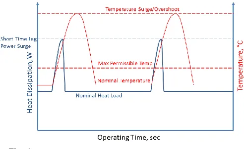
An IGBT (Integrated Gate Bipolar Transistor) inverter is a device used to convert DC voltage into AC voltage. A typical application for these devices is in an electric vehicle (EV) to convert the DC voltage of the battery into AC voltage for the electric motor. During the DC/AC conversion process, heat is released due to inefficiencies of the device. If this heat is not managed, the device can overheat and stop functioning. One of the characteristics of an IGBT inverter is that heat is produced in pulses (Denk and Bakram, 2015). For example, the device can have surges in heat load many times the nominal heat load for a number of seconds. This may make it surpass its maximum permissible temperature as demonstrated in Fig. 1. This makes the thermal management of an IGBT inverter relatively difficult.

Fig. 1 Pulsing nature of IGBT inverters.

When conducting modelling of a heat sink for an IGBT inverter, simple steady state analysis is not appropriate. For example, if an IGBT inverter has a nominal heat load of 60 W, but has pulses of 240 W, for steady state analysis the worst case scenario of 240 W must be modelled.

*_{Corresponding author. Email: bradley.orr@jp.fujikura.com}

If the heat sink must keep the IGBT chip under a certain temperature, this would lead to an oversized heat sink being designed. Most likely the heat sink would be too big and expensive to be viable. To avoid designing an oversized heat sink, transient thermal analysis must be used. Transient thermal analysis takes into consideration the thermal masses of the system, the duration of the heat load and the varying magnitude of the heat load. For the example stated above, transient modelling would show that the peak chip temperatures measured would never reach the calculated steady state modelling temperature. This means a smaller, cheaper heat sink can be viable.

2. TRANSIENT THERMAL MODEL

A transient thermal model was developed for the heat sink shown in Fig. 2. This heat sink was selected because it is an appropriate size for IGBT chip cooling. The transient modelling was done in the form of a thermal resistor/capacitor network. To complete this style of modelling, the component thermal resistances and the corresponding component thermal capacitances need to be determined. The component thermal resistances can be found either experimentally or theoretically. As the heat sink is already available, in this case the thermal resistances were found experimentally. The materials and volume of each component of the heat sink were known therefore each component thermal capacitance can be determined. The component thermal resistances and thermal capacitances determined are shown in table 1. The thermal resistor/capacitor network for the heat sink can be seen in Fig. 3.

Fig. 2 The heat sink modelled (a) and the heat sink schematic (b).

Frontiers in Heat and Mass Transfer

(2)

Table 1 Component thermal resistances and capacitances

𝑅1= 𝑅ℎ𝑒𝑎𝑡𝑒𝑟−𝑏𝑎𝑠𝑒 0.1733°𝐶/𝑊

𝑅2= 𝑅𝑏𝑎𝑠𝑒−𝑓𝑖𝑛𝑠 9.712 × 10−3°𝐶/𝑊

𝑅3= 𝑅𝑓𝑖𝑛𝑠−𝑎𝑖𝑟 0.3054°𝐶/𝑊

𝐶1= 𝐶𝑐𝑜𝑝𝑝𝑒𝑟 ℎ𝑒𝑎𝑡𝑒𝑟 𝑏𝑙𝑜𝑐𝑘 136𝐽/𝐾

𝐶2= 𝐶𝑎𝑙𝑢𝑚𝑖𝑛𝑖𝑢𝑚 𝑏𝑎𝑠𝑒 341𝐽/𝐾

𝐶3= 𝐶𝑎𝑙𝑢𝑚𝑖𝑛𝑖𝑢𝑚 𝑓𝑖𝑛𝑠 159 𝐽/𝐾

Fig. 3 Thermal resistance / capacitor network of the heat sink.

This thermal resistance/capacitor network can be solved using Kirchhoff’s law at each node to derive a number of heat balance equations. Kirchhoff’s law is stated in eq. (1).

𝑄̇𝑖𝑛= 𝑄̇𝑜𝑢𝑡+ 𝑄̇𝑠𝑡𝑜𝑟𝑒𝑑 (1)

The heat balance equation for the heater temperature node is eq. (2). The heat balance equation for the base temperature node is eq. (3). The heat balance equation for the fin temperature node is eq. (4). All three equations are rearranged to make the derivative the subject.

𝑄̇𝑖𝑛= 𝑇ℎ−𝑇𝑏

𝑅1 + 𝐶1𝑇ℎ

′ _(2a)

𝑇ℎ′= 𝑄̇𝑖𝑛

𝐶1 −

𝑇ℎ−𝑇𝑏

𝐶1𝑅1 (2b)

𝑇ℎ−𝑇𝑏

𝑅1 =

𝑇𝑏−𝑇𝑓

𝑅2 + 𝐶2𝑇𝑏

′ _(3a)

𝑇𝑏′= 𝑇ℎ−𝑇𝑏

𝐶2𝑅1 −

𝑇𝑏−𝑇𝑓

𝐶2𝑅2 (3b)

𝑇𝑏−𝑇𝑓

𝑅2 =

𝑇𝑓−𝑇𝑎

𝑅3 + 𝐶3𝑇𝑓

′ _(4a)

𝑇𝑓′= 𝑇𝑏−𝑇𝑓

𝐶3𝑅2 −

𝑇𝑓−𝑇𝑎

𝐶3𝑅3 (4b)

Euler’s method can then be used to solve these equations in an excel spreadsheet. Equations (5-8) below are the Euler’s method equations.

𝑡𝑛+1= 𝑡𝑛+ ℎ (5)

𝑇ℎ𝑛+1= 𝑇ℎ𝑛+ ℎ × 𝑇ℎ𝑛

′ ₍₆₎

𝑇𝑏𝑛+1= 𝑇𝑏𝑛+ ℎ × 𝑇𝑏𝑛

′ ₍₇₎

𝑇𝑓𝑛+1= 𝑇𝑓𝑛+ ℎ × 𝑇𝑓𝑛

′ ₍₈₎

The heat sink is initially at ambient temperature so the initial conditions are known. These initial temperatures can be substituted into eqs. (2-4) to find the temperature gradient at t = 0 s. The initial temperature gradients are then substituted into eqs. (6-8) along with the initial temperatures and a step size of h= 1 s to find the temperatures at t = 1 s. The cycle then repeats itself with the newly calculated temperatures at t = 1 s being substituted into eqs. (2-4). This particular methodology is common for solving thermal resistance/capacitance networks (Mochizuki, 2018; Mochizuki et al., 2018; Mochizuki et al., 2017).

3. VALIDATING THE MODEL

Modelling was conducted under two different sets of conditions. The first condition assumes that everything is initially at the ambient temperature of 25 °C with heat input constant at 120 W. The second condition assumes that everything is initially at the ambient temperature of 25.5 °C with heat input in intervals of 240 W for 30 seconds then 60 W for 60 seconds. A step size of 1 second was used for Euler’s method. Experimental data was obtained using the test set up shown in Fig. 2 previously. For the second condition, a switch was used to manually change from two separate power supplies and enable switching from 60 W to 240 W. Figure 4 shows a comparison of theoretical and experimental data for the first condition. Figure 5 shows a comparison of theoretical and experimental data for the second condition. For the first condition, the maximum ΔT between experimental and theoretical data was approximately 1.5 °C. For the second condition, the maximum ΔT between experimental and theoretical data was approximately 5 °C. The error for the second condition is expected to be higher due to the possibility of the pulses being out of sync. In both cases it can be seen that theoretical and experimental data matches well therefore the transient thermal model is valid.

Fig. 4 Experiment and theory heat sink temps. (First condition).

Fig. 5 Experiment and theory heat sink temps. (Second condition).

0 20 40 60 80 100

0 200 400 600 800 1000

Tem

p

e

ratu

re

(

°C)

Time (s)

Th (experimental) Tb (experimental) Tf (experimental) Ta (experimental) Th (theoretical) Tb (theoretical) Tf (theoretical) Ta (theoretical)

0 20 40 60 80 100

0 500 1000 1500

Tem

p

e

ratu

re

(

°C)

Time (s)

(3)

3

4. TRANSIENT MODELLING OF PHASE CHANGE

MATERIAL (PCM)

Phase change material (PCM) is used to absorb heat or release heat at a constant temperature. Typically PCM is used in situations where it changes from solid to liquid and vice versa. When PCM is below its melting point temperature, as heat is added the temperature of the PCM will increase. When the PCM reaches the melting point temperature, as heat is added the temperature remains constant until all the PCM has melted. Only after all the PCM has melted will the temperature begin to rise with continuing heat input. This phenomenon is demonstrated in Fig. 6 (Evans et al., 2001). PCM has been used in applications such as latent heat storage (Khalifa et al., 2016) and passively reducing the peak temperature of objects (Tan et al., 2011; Tan et al., 2011). PCM typically has a low thermal conductivity which negatively effects performance but improvements to the thermal conductivity of PCM has been demonstrated by adding nano particles and/or fin structures (Alizadeh et al., 2019; Alizadeh et al., 2019; Hosseinzadeh et al., 2019; Hosseinzadeh et al., 2019; Singh et al., 2018; Valan Arasu et al., 2011). The use of PCM in combination with a heat sink also has the ability to reduce peak temperatures of an IGBT chip.

Fig. 6 The effect of PCM (Evans et al., 2001).

A limitation of transient thermal models using thermal resistance/capacitor networks is that these types of models only consider sensible heat storage. They don’t consider latent heat storage as in the case of PCM. The use of PCM in a system has the same effect as adding more thermal capacitance. The difference is this effect is temporary until all the PCM has melted. Assumptions can be made to enable modelling PCM as a temporary thermal capacitance. Equations (9a-c) are used to derive the effective temporary thermal capacitance of PCM. For a thermal mass to absorb heat it must increase in temperature. Therefore, an assumption is made that phase change occurs over a small temperature difference. Other assumptions made to simplify modelling are PCM has no effect on thermal resistance, PCM has no effect on sensible heat transfer and that the PCM temperature is uniform. PCM melting / solidifying temperature hysteresis is assumed to be negligible (Komatsu et al., 2013; Usami et al., 2014).

For an example, an assumption is made that PCM is placed in the fin location of the previously modelled heat sink. In this example, a paraffin wax with thermophysical properties such as 144 kJ/kg for latent heat and 60 °C melting point are used. Assuming 30 g of this paraffin wax is used, its effective temporary thermal capacitance is calculated using eqs. (9d-e). Phase change is assumed to occur from 60 °C to 62 °C (ΔT = 2 °C). When modelling this problem, the extra thermal capacitance of the PCM is only added when the fin temperature is between 60 °C to 62 °C. This is described by table 2.

𝑄𝑝ℎ𝑎𝑠𝑒𝑐ℎ𝑎𝑛𝑔𝑒= 𝑄𝑃𝐶𝑀𝑡ℎ𝑒𝑟𝑚𝑎𝑙𝑚𝑎𝑠𝑠 (9a)

ℎ𝑙𝑎𝑡𝑒𝑛𝑡× 𝑚𝑃𝐶𝑀= 𝐶𝑃𝐶𝑀× ∆𝑇 (9b)

𝐶𝑃𝐶𝑀=

ℎ𝑙𝑎𝑡𝑒𝑛𝑡×𝑚𝑃𝐶𝑀

∆𝑇 (9c)

𝐶𝑃𝐶𝑀=

(144×103_)×0.030

2 (9d)

𝐶𝑃𝐶𝑀= 2205 𝐽

𝐾 (9e)

Table 2 Component thermal resistances and capacitances (with PCM)

𝑅1= 𝑅ℎ𝑒𝑎𝑡𝑒𝑟−𝑏𝑎𝑠𝑒 0.1733°𝐶/𝑊

𝑅2= 𝑅𝑏𝑎𝑠𝑒−𝑓𝑖𝑛𝑠 9.712 × 10−3°𝐶/𝑊

𝑅3= 𝑅𝑓𝑖𝑛𝑠−𝑎𝑖𝑟 0.3054°𝐶/𝑊

𝐶1= 𝐶𝑐𝑜𝑝𝑝𝑒𝑟 ℎ𝑒𝑎𝑡𝑒𝑟 𝑏𝑙𝑜𝑐𝑘 136 𝐽/𝐾

𝐶2= 𝐶𝑎𝑙𝑢𝑚𝑖𝑛𝑖𝑢𝑚 𝑏𝑎𝑠𝑒 341 𝐽/𝐾

𝐶3= 𝐶𝑎𝑙𝑢𝑚𝑖𝑛𝑖𝑢𝑚 𝑓𝑖𝑛𝑠 159𝐽/𝐾 𝑤ℎ𝑒𝑛𝑇ℎ< 60,𝑇ℎ> 62

2364 𝐽/𝐾 𝑤ℎ𝑒𝑛60 ≤ 𝑇ℎ≤ 62

Figure 7 shows a comparison of the heat sink modelling data with PCM material and without PCM material. In this case the heat input was constant at 200 W. It can be seen that when the fin temperature reaches 60 °C, the temperature rise starts to slow. This is because the PCM has started melting so the temporary extra thermal capacitance is added. After the fin temperature reaches 62 °C, the PCM has completely melted so the thermal capacitance is returned to normal and the fin temperature rise returns to normal. The shape of the temperature curve is very similar to curve shown in Fig. 6. This demonstrates that it is possible to model PCM with thermal resistance / capacitor networks.

Fig. 7 Theoretical temperatures of the heat sink with / without PCM.

5. OPTIMISATION OF PCM

Now that the effect of PCM can be modelled, this model can be used optimise the use of PCM. In this case, optimisation of PCM location, melting temperature and mass can be undertaken. In tables 3-5, the parameters used in the model when optimising PCM locations are shown. Constant parameters are 30 g of PCM is used and the melting temperature is 60 °C. The same power input as Fig. 5 is used. It can be seen that the extra PCM capacitance is added to either C1, C2, or C3 depending on the PCM location. Figures 8-10 are the model output in these 3 situations. In Fig. 8 the PCM is located at the heater. In this situation, as soon as the heater reaches 60 °C, the PCM starts melting and the heater temperature rise is delayed. After all the PCM has melted, the cyclic temperature variation returns to normal. In Fig. 9 the PCM is located at the base. This

0

20

40

60

80

100

120

0

100

200

300

400 Te

mpe

ra

tu

re

(

°C)

Time (s)

Th (no PCM)

Tb (no PCM)

Tf (no PCM)

Ta (no PCM)

Th (with PCM)

Tb (with PCM)

(4)

figure shows when the base temperature reaches 60 °C, the base temperature fluctuations start to flatten. From these results it seems there is little effect on heater temperature fluctuations. In Fig. 10 the PCM is located at the fins. When the fins reach 60 °C, the fin temperature fluctuations start to flatten but also in this case there seems to be very little effect on heater temperature variation. Figure 11 shows the heater temperature of all 3 cases. From these results it can be clearly seen that the only time the PCM has an effect is when the PCM is located at the heater. It seems the PCM should be located as close to the heat source as possible. Therefore moving forward, modelling will be conducted using PCM at the heater.

Table 3 Parameters when optimising PCM location (PCM at heater)

𝑅1 0.1733°𝐶/𝑊

𝑅2 9.712 × 10−3°𝐶/𝑊

𝑅3 0.3054°𝐶/𝑊

𝐶1 136𝐽/𝐾 𝑤ℎ𝑒𝑛𝑇ℎ< 60,𝑇ℎ> 62

2341 𝐽/𝐾 𝑤ℎ𝑒𝑛60 ≤ 𝑇ℎ≤ 62

𝐶2 341𝐽/𝐾

𝐶3 159 𝐽/𝐾

Table 4 Parameters when optimising PCM location (PCM at base)

𝑅1 0.1733°𝐶/𝑊

𝑅2 9.712 × 10−3°𝐶/𝑊

𝑅3 0.3054°𝐶/𝑊

𝐶1 136 𝐽/𝐾

2546 𝐽/𝐾 𝑤ℎ𝑒𝑛60 ≤ 𝑇ℎ≤ 62

𝐶3 159 𝐽/𝐾

Table 5 Parameters when optimising PCM location (PCM at fins)

𝑅1 0.1733°𝐶/𝑊

𝑅2 9.712 × 10−3°𝐶/𝑊

𝑅3 0.3054°𝐶/𝑊

𝐶1 136 𝐽/𝐾

𝐶2 341 𝐽/𝐾

2364 𝐽/𝐾 𝑤ℎ𝑒𝑛60 ≤ 𝑇ℎ≤ 62

Fig. 8 PCM at heater.

Fig. 9 PCM at base.

Fig. 10 PCM at fins.

Fig. 11 Optimising PCM location.

0

20

40

60

80

100

0

500 1000

1500

Te

mpe

ra

tu

re

(

°C)

Time (s)

Th

Tb

Tf

Ta

0

20

40

60

80

100

0

500 1000

1500

Te

mpe

ra

tu

re

(

°C)

Time (s)

Th

Tb

Tf

Ta

0

20

40

60

80

100

0

500 1000

1500

Te

mpe

ra

tu

re

(

°C)

Time (s)

Th

Tb

Tf

Ta

0

20

40

60

80

100

0

500 1000

1500

Te

mpe

ra

tu

re

(

°C)

Time (s)

(5)

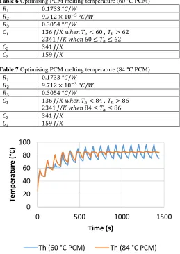
5 After the optimum PCM location has been found, the optimum PCM melting temperature can be determined. In this case, PCM with melting points of 60 °C and 84 °C were considered. 84 °C PCM was considered because the average heater saturation temperature is 84 °C. The only variable in this comparison is the melting point. The PCM mass and location are constant. In reality PCM of different melting points would be a different material with different latent heat but for the purpose of this simulation the latent heat is unchanged. Tables 6 and 7 show the modelling parameters for this comparison. Figure 12 is the output of the model when using these parameters. From the previous Fig. 11 it is known that the 60 °C PCM has little effect on heater temperature at saturation. This is also shown in Fig. 12. However Fig. 12 demonstrates that the use of 84 °C PCM seems to have a significant reduction of peak temperatures at saturation. Therefore moving forward, modelling will be conducted using 84 °C PCM.

Table 6 Optimising PCM melting temperature (60 °C PCM)

𝑅1 0.1733°𝐶/𝑊

𝑅2 9.712 × 10−3°𝐶/𝑊

𝑅3 0.3054°𝐶/𝑊

2341 𝐽/𝐾 𝑤ℎ𝑒𝑛60 ≤ 𝑇ℎ≤ 62

𝐶2 341𝐽/𝐾

𝐶3 159 𝐽/𝐾

Table 7 Optimising PCM melting temperature (84 °C PCM)

𝑅1 0.1733°𝐶/𝑊

𝑅2 9.712 × 10−3°𝐶/𝑊

𝑅3 0.3054°𝐶/𝑊

2341 𝐽/𝐾 𝑤ℎ𝑒𝑛84 ≤ 𝑇ℎ≤ 86

𝐶2 341𝐽/𝐾

𝐶3 159 𝐽/𝐾

Fig. 12 Optimising PCM melting temperature.

The final parameter to be optimised is the PCM mass. In this case, 10 g, 30 g and 90 g were considered. Similarly to the previous modelling, the only parameter that is changed is the PCM mass. The PCM location and melting temperature are constant. Tables 8-10 show the modelling parameters for this comparison. Figure 13 is the output of the modelling. From these results it seems that 10 g of PCM is insufficient because the PCM fully melts and solidifies very quickly and temperature peaks and troughs are still observed. There seems to very little difference when 30 g or 90 g are used. This is because in both cases the PCM is continuously undergoing phase change. Therefore in this case 30 g of PCM is optimum because any extra PCM would be unnecessary and increase the cost.

Table 8 Parameters when optimising PCM mass (10 g PCM)

𝑅1 0.1733°𝐶/𝑊

𝑅2 9.712 × 10−3°𝐶/𝑊

𝑅3 0.3054°𝐶/𝑊

871 𝐽/𝐾 𝑤ℎ𝑒𝑛84 ≤ 𝑇ℎ≤ 86

𝐶2 341𝐽/𝐾

𝐶3 159 𝐽/𝐾

𝑅1 0.1733°𝐶/𝑊

𝑅2 9.712 × 10−3°𝐶/𝑊

𝑅3 0.3054°𝐶/𝑊

2341 𝐽/𝐾 𝑤ℎ𝑒𝑛84 ≤ 𝑇ℎ≤ 86

𝐶2 341𝐽/𝐾

𝐶3 159 𝐽/𝐾

𝑅1 0.1733°𝐶/𝑊

𝑅2 9.712 × 10−3°𝐶/𝑊

𝑅3 0.3054°𝐶/𝑊

6751 𝐽/𝐾 𝑤ℎ𝑒𝑛84 ≤ 𝑇ℎ≤ 86

𝐶2 341𝐽/𝐾

𝐶3 159 𝐽/𝐾

Fig. 13 Optimising PCM mass.

Now that the PCM location, melting temperature and mass have been optimised, this data can be compared to the modelling without any PCM. From Fig. 14 it can be seen that when optimum PCM is used, there is a potential to reduce peak temperatures at saturation by approximately 10.27 °C. When the power input and duration changes, the optimum parameters would also change but nonetheless this modelling shows the potential of PCM in reducing peak IGBT temperatures.

If a result similar to what is shown in Fig. 14 can be obtained in reality, this would be a significant improvement. Reducing the peak temperatures of any type of integrated circuit is widely known to improve the operating efficiency and device lifetime. In addition to this, it is known that smaller temperature fluctuations can improve device lifetime. In this particular case, the temperature fluctuation at saturation has improved from approximately ±10 °C with no PCM to approximately ±2 °C with optimum PCM.

0

20

40

60

80

100

0

500 1000

1500

Te

mpe

ra

tu

re

(

°C)

Time (s)

Th (60 °C PCM)

Th (84 °C PCM)

0

20

40

60

80

100

0

500 1000

1500

Te

mpe

ra

tu

re

(

°C)

Time (s)

(6)

Fig. 14 No PCM vs optimum PCM.

6. CONCLUSIONS

Transient thermal modelling was conducted on a heat sink with the intended application of cooling an IGBT inverter chip. Transient thermal modelling was required due to the pulse heat input characteristics of the IGBT chip. The modelling data was compared with experimental data and was found to be valid. The use of PCM with the heat sink was identified as a potential method to reduce peak chip temperatures. It has been shown that it is possible to model PCM in a thermal resistance / capacitor network. Modelling demonstrates that the PCM should be located as close to the heat source as possible. The optimum PCM melting temperature should be close to the average heat source temperature at saturation. The optimum amount of PCM would be the minimum amount of PCM required for phase change to continuously occur. Any extra PCM would have the same performance so would be unnecessary. Future work would be to validate the modelling considering PCM.

NOMENCLATURE

𝐶 Thermal capacitance (J/K)

ℎ Euler’s method step size (s)

ℎ𝑙𝑎𝑡𝑒𝑛𝑡 Latent heat of fusion (J/kg)

𝑚 Mass (kg)

𝑄 Heat energy (J)

𝑄̇ Heat transfer rate (W)

𝑅 Thermal resistance (°C/W)

𝑡 Time (s)

𝑇𝑎 Ambient temperature (°C)

𝑇𝑏 Base temperature (°C)

𝑇𝑓 Fin temperature (°C)

𝑇ℎ Heater temperature (°C)

𝑇′ _{Rate of temperature change (}_°_C/s)

∆𝑇 Temperature difference (°C)

REFERENCES

Alizadeh, M., Hosseinzadeh, K., Ganji, D., 2019, “Investigating the effects of hybrid nanoparticles on solid-liquid phase change process in a Y-shaped fin-assisted LHTESS by means of FEM,” Journal of Molecular Liquids, 287, 110931.

https://doi.org/10.1016/j.molliq.2019.110931

Alizadeh, M., Hosseinzadeh, K., Mehrzadi, H., Ganji, D., 2019, “Investigation of LHTESS filled by Hybrid nano-enhanced PCM with Koch snowflake fractal cross section in the presence of thermal radiation,” Journal of Molecular Liquids, 273, pp 414-424.

https://doi.org/10.1016/j.molliq.2018.10.049

Denk, M., and Bakran, M.M., 2015, “Online Junction Temperature Cycle Recording of an IGBT Power Module in a Hybrid Car,” Advances in Power Electronics, 2015, 652389.

http://dx.doi.org/10.1155/2015/652389

Evans, A.G., He, M.Y., Hutchinson, J.W., and Shaw, M., 2001, “Temperature distributions in advanced power electronics systems and the effect of phase change materials on temperature suppression during power pulses,” Journal of electronic packaging, 123(3), pp 211-217.

http://doi.org/10.1115/1.1370376

Hosseinzadeh, K., Alizadeh, M., Ganji, D., 2019, “Solidification process of hybrid nano-enhanced phase change material in a LHTESS with tree-like branching fin in the presence of thermal radiation,” Journal of Molecular Liquids, 275, pp 909-925.

https://doi.org/10.1016/j.molliq.2018.11.109

Hosseinzadeh, K., Alizadeh, M., Tavakoli, M., Ganji, D., 2019, “Investigation of phase change material solidification process in a LHTESS in the presence of fins with variable thickness and hybrid nanoparticles,” Applied Thermal Engineering, 152, pp 706-717.

https://doi.org/10.1016/j.applthermaleng.2019.02.111

Khalifa, A., Tan, L., Mahony, D., Date, A., and Akbarzadeh, A., 2016, “Numerical analysis of latent heat thermal energy storage using miniature heat pipes: A potential thermal enhancement for CSP plant development,” Applied Thermal Engineering, 108, pp 93-103.

https://doi.org/10.1016/j.applthermaleng.2016.07.111

Komatsu, S., Komiyama, S., Ookubo, A., and Kanae, A., 2013, “Development of the Latent Heat Material CALGRIP for Temperature Management Transportation,” JSR technical review, No.120.

Mochizuki, M., 2018, “Thermal Analysis and Design of Li-ion Battery with safety Function to protect temperature Over shoot,” The Japan Institute of Electronics Packaging Conference, Tokyo, Japan.

Mochizuki, M., Shimizu, H., Kato, T., Kawaguchi, M., Arai, H., Nguyen, T., Nguyen, T., and van Raay, T., 2018, “Thermal Analysis and Design of In Wheel Motor for Electric Vehicle,” #55 Japan Symposium of Heat Transfer, Sapporo, Japan.

Mochizuki, M., Ohashi, M., Hagino, H., Kawahara, Y., and Saito, Y., 2017, “Development of PTC Thin Film for Li ion Battery to protect temperature Over-rise,” #54 Japan Symposium of Heat Transfer, Ohmiya, Japan.

Singh, R., Sadeghi, S., Shabani, B., 2018, “Thermal Conductivity of Phase Change Materials for Low-Temperature Thermal Energy Storage Applications,” Energies, 12(1), 75.

https://doi.org/10.3390/en12010075

Tan, L., Date, A., Date, A., and Akbarzadeh, A., 2011, “Experimental investigation of cooling effect on photovoltaic panel using phase change material,” CET conference proceedings, Shanghai, China, pp 260-263. Tan, L., Singh, R., Date, A., Akbarzadeh, A., 2011, “Thermal performance of two-phase closed thermosiphon in application of concentrated thermoelectric power generator using phase change material thermal storage,” Frontiers in Heat Pipes, 2, 043001.

http://dx.doi.org/10.5098/fhp.v2.4.3001

Usami, H., Miura, M., and Ishidoya, Y., 2014, “A Study on the Efficiency of Latent Thermal Storage for Air-Conditioning System with Granulated Phase Change Material”.

Valan Arasu, A., Sasmito, A., Mujumdar, A., 2011, “Thermal performance enhancement of paraffin wax with AL2O3 and CuO nanoparticles – A numerical study,” Frontiers in Heat and Mass Transfer, 2(4), 043005.