Spatial aliasing and distortion of energy distribution in the wave vector domain under multi-spacecraft measurements

www.ann-geophys.net/27/3031/2009/

© Author(s) 2009. This work is distributed under the Creative Commons Attribution 3.0 License.

Annales

Geophysicae

Spatial aliasing and distortion of energy distribution in the wave

vector domain under multi-spacecraft measurements

Y. Narita1and K.-H. Glassmeier1,2

1_{Institut f¨ur Geophysik und extraterrestrische Physik, Mendelssohnstr. 3, 38106 Braunschweig, Germany} 2_{Max-Planck-Institut f¨ur Sonnensystemforschung, Max-Planck-Str. 2, 37191 Katlenburg-Lindau, Germany} Received: 7 May 2009 – Revised: 27 July 2009 – Accepted: 27 July 2009 – Published: 5 August 2009

Abstract. Aliasing is a general problem in the analysis of any measurements that make sampling at discrete points. Sampling in the spatial domain results in a periodic pattern of spectra in the wave vector domain. This effect is called spatial aliasing, and it is of particular importance for multi-spacecraft measurements in space. We first present the theo-retical background of aliasing problems in the frequency do-main and generalize it to the wave vector dodo-main, and then present model calculations of spatial aliasing. The model cal-culations are performed for various configurations of the re-ciprocal vectors and energy spectra or distribution that are placed at different positions in the wave vector domain, and exhibit two effects on aliasing. One is weak aliasing, in which the true spectrum is distorted because of non-uniform aliasing contributions in the Brillouin zone. It is demon-strated that the energy distribution becomes elongated in the shortest reciprocal lattice vector direction in the wave vec-tor domain. The other effect is strong aliasing, in which aliases have a significant contribution in the Brillouin zone and the energy distribution shows a false peak. These results give a caveat in multi-spacecraft data analysis in that spectral anisotropy obtained by a measurement has in general two ori-gins: (1) natural and physical origins like anisotropy imposed by a mean magnetic field or a flow direction; and (2) aliasing effects that are imposed by the configuration of the measure-ment array (or the set of reciprocal vectors). This manuscript also discusses a possible method to estimate aliasing contri-butions in the Brillouin zone based on the measured spectrum and to correct the spectra for aliasing.

Keywords. Electromagnetics (Antenna arrays; Signal pro-cessing and adaptive antennas) – Space plasma physics (Ex-perimental and mathematical techniques)

Correspondence to: Y. Narita

([email protected])

1 Introduction

Recent progress in our understanding of near-Earth space environments such as the solar wind or the Earth’s mag-netosphere benefits greatly from multi-spacecraft missions that enable us to distinguish between temporal and spatial variations in the observations, and allows us to determine three-dimensional structures in space. The Cluster mission (Escoubet et al., 2001; Balogh et al., 2001) performs four-point measurements with its tetrahedron configuration and the THEMIS mission (Angelopoulos, 2008; Auster et al., 2008) performs five point measurements. There exist a num-ber of data analysis methods that are developed particularly for such multi-point measurements, parts of which are sum-marized in Glassmeier et al. (1995) and Paschmann and Daly (1998, 2008). One of the unique and powerful anal-ysis methods in studying dynamics of space plasma is to determine the energy distribution directly in the wave vec-tor domain, referred to as the wave telescope technique (or k-filtering) (Neubauer and Glassmeier, 1990; Pinc¸on and Lefeuvre, 1991; Motschmann et al., 1996; Glassmeier et al., 2001). This technique is based on the minimum variance method of Capon (1969) estimating the energy spectrum or distribution in the frequency and wave vector domain using only several points of measurements.

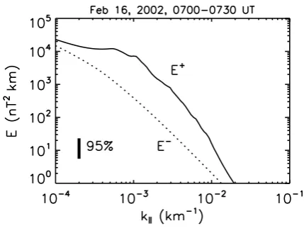
Fig. 1. Example of anisotropic energy spectrum as a function of

the wave number parallel to the mean magnetic field, taken from the Cluster observation in the shock-upstream region after Narita et al. (2007). The solid curve represents the spectrum for magnetic field fluctuations in the direction away from the bow shock (E+) and the dotted curve represents that in the direction toward the bow shock (E−).

from the sun toward the shock (E−_{). While the larger energy}

contribution inE+can be physically interpreted as the ex-citation of the waves propagating away from the bow shock, one may also ask how important the aliasing effect is in eval-uating the energy spectrum.

It is worthwhile to note that spatial structures can not al-ways be resolved and identified in the multi-point measure-ments. For example, one can not identify the spatial struc-ture when its characteristic scale (e.g. wavelength) is smaller than the sensor separation distance. In that case the measure-ment makes under-sampling and the result is subject to alias-ing problem. Neubauer and Glassmeier (1990) presented the concept of spatial aliasing under multi-point measurements in space, and measurements using the four Cluster spacecraft indeed suggest the existence of spatial aliasing (Sahraoui et al., 2003; Tjulin et al., 2005).

The configuration of the sensor array can be represented as a set of reciprocal vectors in the wave vector domain, and the analysis in the wave vector domain can be performed within the first Brillouin zone or Wigner-Seitz cell (hereafter referred to as the Brillouin zone or simply the cell) spanned by the half-length reciprocal vectors (Kittel, 1996). Beyond the Brillouin zone the determined spatial structures do not reflect the true structure any more, instead its aliases appears periodically in the wave vector domain.

Aliasing is a general problem not only in science but also in engineering so far as discrete measurements sample a con-tinuous function. The goals of this paper are (1) to general-ize aliasing theory from the frequency domain to the wave vector domain, and (2) demonstrate various cases of spatial aliasing in the wave vector domain. It is concluded that the

configuration of sensor arrays may significantly influence the measurement of spatial structures due to the aliasing problem even though the analysis is limited within the Brillouin zone. We also discuss a remedy to correct for the aliasing part in the measurement.

2 Theoretical background

2.1 Sampling formulas in time domain

Sampling formulas, their mathematical foundation, and the aliasing problem have been developed and studied in a num-ber of papers, not only in the celebrated work of Nyquist (1928) and Shannon (1949) but also in recent papers such as Unser (2000) and Kirchner (2005). We briefly discuss the relation between sampling in the time domain and the associ-ated aliasing in the frequency domain. This is essentially an aliasing problem in a one-dimensional system and provides a basis for understanding the aliasing in the wave vector do-main.

Spectral aliasing in some under-sampled time series can be understood in the following fashion. Consider a continuous functiong(t )in the time domain and its Fourier transform G(f )in the frequency domain. The functiong(t )is mea-sured at discrete points, yielding our sampled signalh(t ) h(t )=g(t )III(t ), (1) where III(t )is called the comb distribution (Bracewell, 2000) which represents an array of delta functions

III(t )= ∞

X

m=−∞

δ(f0t−m). (2) Here f0 denotes the sampling rate f0=1/1t. The comb distribution is a periodic function and can be expressed as a Fourier series

III(t )= ∞

X

n=−∞

cnei2π nf0t. (3) Furthermore, it turns out that the Fourier coefficientscnare all unity:

cn= 1 1t

Z 1t₂

−1t

2

δ(f0t )e−i2π nf0tdt=1, (4) where one of the properties of the delta function,δ(f0t )= δ(t )/f0was used. The Fourier transform of the sampled sig-nalh(t )is obtained by combining Eqs. (1), (3), and (4). H (f )=

Z ∞

−∞

h(t )e−i2πf0tdt (5)

=

Z ∞

−∞

g(t )III(t )e−i2πf0t_{dt (6)}

= ∞

X

n=−∞

Z ∞

−∞

= ∞

X

n=−∞

G(f−nf0). (8)

In the last equation one sees the essence of the aliasing prob-lem, that is the Fourier transform of the sampled signal con-tains not only the Fourier transform of the original func-tionG(f )but also contributions from then-th harmonics of the sampling frequencyG(f−nf0). The power spectrum is proportional to the expectation value of the squared Fourier transform. On the assumption that the phase between any two frequency components is random, the power spectrum is also a sum of the respective alias component,

P (f )=E

h

|H (f )|2

i

= ∞

X

n=−∞

|G(f−nf0)|2, (9)

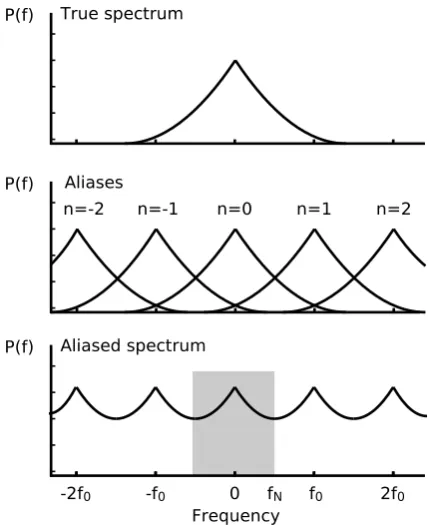
where the symbolE[···]denotes the operation of the expec-tation value. Figure 2 displays the periodic pattern of power spectrum. In this example the contribution from aliases is significant and the true spectrum (top panel) becomes en-hanced and distorted in the aliased spectrum (bottom panel) that takes account of the true spectrum and its alias contribu-tions, even within the Nyquist frequencyfN=f0/2. 2.2 Sampling formulas in spatial domain

The above sampling formulas can be generalized to the spa-tial domain. Consider now a continuous function of vector in real space,g(r), and its Fourier transform in the wave vec-tor domain, G(k). The sampled signal is a filtering of the functiong(r)by the set of the delta functions III(r), namely h(r)=g(r)III(r). (10) The comb distribution in the spatial domain is expressed as III(r)= ∞ X m3=−∞ ∞ X m2=−∞ ∞ X m1=−∞ δ _k

3·r 2π −m3

δ

_k

2·r 2π −m2

δ

_k

1·r 2π −m1

(11)

= ∞

X

m3=−∞ δ

_k

3·r 2π −m3

∞

X

m2=−∞ δ

_k

2·r 2π −m2

∞ X m1=−∞ δ _k

1·r 2π −m1

(12)

or as a Fourier series III(r)=

∞

X

n3=−∞

ein3k3·r

∞

X

n2=−∞

ein2k2·r

∞

X

n1=−∞

ein1k1·r ₍₁₃₎

= ∞ X n3=−∞ ∞ X n2=−∞ ∞ X n1=−∞

ei(n1k1+n2k2+n3k3)·r_{, (14)}

wherek1,k2, andk3are the reciprocal vectors of the primi-tive vectors of the sensor array (or spacecraft separation vec-tors)r1,r2, andr3. Equation (12) is a grouping of the sums

Fig. 2. Illustration of aliasing in the frequency domain. A true spectrum (top panel) appears periodically as aliases in the frequency domain with the frequency shiftnf0(middle panel). This results in distortion of the original spectrum (bottom panel) even within the Nyquist frequencyfN(shaded area).

in Eq. (11) with respect tom1,m2, andm3. Equation (13) is obtained by Fourier series expansion of the three delta func-tions in Eq. (12) (cf. Eqs. 2–4). Equation (14) combines three exponential functions in Eq. (13) together.

The reciprocal vectors are obtained by the primitive vec-torsr1,r2, andr3as

k1=2π

r2×r3 r1·(r2×r3)

(15) k2=2π

r3×r1 r2·(r3×r1)

(16) k3=2π

r1×r2 r3·(r1×r2)

, (17)

satisfying the orthogonality condition:

ki·rj=2π δij, (18)

whereδijrepresents Kronecker’s delta. The set of these three reciprocal vectors used in this study are the canonical choice in solid state physics. An alternative set of reciprocal vectors is also in use (Chanteur, 1998). The Fourier transform of h(r)is given as

H (k)=

Z

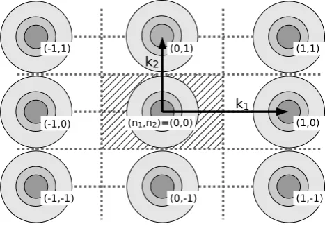
Fig. 3. Aliasing in the wave vector domain. The shaded disks

rep-resent the energy distribution with its aliases. The hatched area with dash-lines is the first Brillouin zone (Wigner-Seitz cell) spanned by the half-length reciprocal vectors.

= X

n1,n2,n3

Z

g(r)e−i(k−n1k1−n2k2−n3k3)·r_d3_{r (20)}

= X

n1,n2,n3

G(k−n1k1−n2k2−n3k3) (21)

Again on the assumption of random phase, one obtains the spectrum in the wave vector domain as

P (k)=Eh|H (k)|2i (22)

= X

n1,n2,n3

|G(k−n1k1−n2k2−n3k3)|2 (23)

Therefore the spatial sampling results in a periodic struc-ture of the spectrum in the wave vector domain, containing both the true spectrum|G(k)|2and its aliases|G(k−n1k1− n2k2−n3k3)|2. Figure 3 displays an illustration of the spec-trum with aliasing in the wave vector domain.

As Neubauer and Glassmeier (1990) state, the periodic structure in the wave vector domain is avoided if we restrict the analysis to a small subvolume of the wave vector space. For example, one can use a sphere in the wave vector do-main with the radius equal to the minimum reciprocal vector length, or one can use a right square or cube with this length. It is important that the analysis should be limited to within the Brillouin zone, otherwise the spectrum exhibits a peri-odic alias pattern in the wave vector domain. However, we stress here that the original spectrum may be enhanced and distorted as shown in Fig. 2 even if we restrict ourselves to the Brillouin zone.

3 Aliasing in the wave vector domain

3.1 An example

Figure 4 displays an example of aliasing in a two-dimensional wave vector domain. The data (the true spec-trum) are generated numerically and the associated aliasing effect is studied. The wave vector domain is spanned by the half-length reciprocal vectorsk1=(0.02,0.00)km−1and k2=(0.00,0.01)km−1. The true spectrum (left panel) repre-sents an isotropic energy distribution, centered almost at the origin(kx,ky)=(0.0001,0.000)km−1and decaying toward larger wave numbers by a power-lawP (|k|)∝k−α with the indexα=5/3. Contribution from the nearest neighboring aliases with(n1,n2)=(±1,±1), (0,±1), (±1,0) in the first Brillouin zone is displayed in the middle panel. A large part of the alias contribution comes from the alias(n1,n2)=(0,1) and(0,−1), since the magnitude of the second reciprocal vectork2 is smaller than that of the first one and the alias partnersG(k−n1k1−n2k2)are spaced in the wave vector domain more closely to each other in the direction tok2. The right panel in Fig. 4 displays the aliased spectrum which is a sum of the true spectrum (left panel) and the aliased part (middle panel). The aliased spectrum is what we expect to obtain from multi-point measurements. It is interesting that the aliased spectrum does not present an isotropic distribu-tion any more, but is elongated in the direcdistribu-tion tok2which is the shortest lattice vector direction in the reciprocal space. It is clear at this stage that the elongation or anisotropy in the energy spectrum or distribution is imposed by the the con-figuration of the reciprocal vectors, especially how close or different the magnitudes of the vectors|k1|and|k2|are from each other. Another effect is that the spectrum is enhanced at various positions in the Brillouin zone. On the other hand, the isotropy in the spectrum is only slightly broken around the peak. The reason for this is that the spectral energy is larger near the peak and furthermore it is at enough distance from the border of the Brillouin zone such that the contribu-tion from the aliases is the smallest there.

Distortion of the spectrum due to aliasing is investigated using two parameters: an enhancement parameterEand an anisotropy parameterA. The enhancement parameter is de-fined as a ratio of the aliased spectrumPalsto the true spec-trum Ptrue as a function of wave number from the spectral peak in a given direction,

E(k)= Pals(k) Ptrue(k)

. (24)

Fig. 4. True spectrum (left), aliased part from the neighboring cells (middle), and aliased spectrum that is a sum of the true spectrum and its

aliases (right).

Table 1. Enhancement parameter and anisotropy parameter in the

example case.

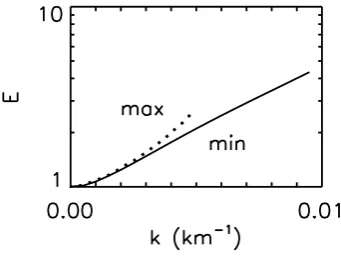
k(km−1) 0.0000 0.0020 0.0040 max(E) 1.00 1.26 1.99

min(E) 1.00 1.25 1.77

A(%) 0 2 12

k=0.0048 km−1. In the minimum enhancement direction it also increases but more moderately than in the maximum di-rection,E=1.00 at the spectral peak,E=2.02 at 0.0048 km−1, andE=4.34 at 0.095 km−1. Some more values of the en-hancement parameter are listed in Table 1 and plotted in Fig. 5.

We then investigate the aliased spectrum with the anisotropy parameter that measures a relative difference in the aliased spectrum between the maximum and the mini-mum enhancement directions:

A=max(Pals)−min(Pals) min(Pals)

. (25)

Alternatively one may use the enhancement parameterE= Pals/Ptrueinstead of the aliased spectrumPalsif the true spec-trum is isotropic, i.e.,Ptrueis independent from the choice of direction from the spectral peak and only a function of the magnitude of the wave number. We evaluate the anisotropy parameter at two different wave numbers (Table 1 bottom). Anisotropy increases as the wave number becomes larger, up toA=24% at the largest wave number available in the max-imum enhancement direction, which is k=0.0048 km−1 (at the right edge of the “max” curve in Fig. 5).

Fig. 5. Enhancement parameter (ratio of aliased to true spectrum)

in the maximum (dotted line) and minimum distortion directions (solid line) for the spectrum in Fig. 4. The x-axis measures distance from the peak of the spectrum in the wave number domain.

3.2 Effect of spectral peak positions and reciprocal vectors

Here we study how aliasing affects the true spectrum under different conditions: (case 1) the peak position is shifted in the true spectrum; (case 2) the lengths of the reciprocal vec-tors are changed for the rectangular Brillouin zone; (case 3) the shape of the Brillouin zone is changed from a rectangular to a diamond-shaped cell; and (case 4) the peak position is shifted in the diamond-shaped cell.

Case 1: Peak position

Fig. 6. Aliased spectra in the wave vector domain including both the true and the aliases spectrum for different peak positions of the true

spectrum shifted in the Brillouin zone. Peak near the origin (left), at an intermediate distance to the border of the Brillouin zone (middle), near the border (right). Reciprocal vectors are orthogonal to each other and the Brillouin zone forms a rectangular cell.

kc=(0.0015,0.0015)km−1in case (1a); at an intermediate distance from the origin and the border of the Brillouin zone, (0.0030,0.0030)km−1, in case (1b); and almost at the border at(0.0045,0.0045)km−1in case (1c).

In all three cases the distribution can be divided into two parts: the distribution is isotropic near the peak, and anisotropic in its surrounding in the sense that the contour lines are elongated and aligned with the shortest lattice vec-tor direction, parallel to k2. In case (1a), the distribution exhibits a distortion in the lower half plane in the Bril-louin zone, a neck-shaped contour line, due to the alias from (n1,n2)=(0,−1). In case (1b), the peak is shifted closer to the upper border of the Brillouin zone. The top part of the true spectrum is not measurable any more as it is beyond the Brillouin zone. Instead its alias(n1,n2)=(0,−1)enters the Brillouin zone. This part of the spectrum corresponds to the missing part of the spectrum at the top of the Brillouin zone. In case (1c), the peak is again shifted even closer to the border of the Brillouin zone. The distribution exhibits now two peaks, one at the top of the cell (which reflects the orig-inal spectrum) and the other at the bottom which is the alias (n1,n2)=(0,−1). The transition from the case (1a) to (1c) suggests that the true spectrum is distorted and elongated un-der a moun-derate alias contribution, while a false peak appears from the opposite side of the Brillouin zone under strong aliasing. The elongation is roughly aligned with the short-est lattice vector direction, and the distortion of the spectrum is largest where the aliasing contribution is largest in the Bril-louin zone.

Case 2: Rectangular cell shape

Not only the peak position but also the shape of the Bril-louin zone is important in the spatial aliasing. Figure 7 compares three different rectangular Brillouin zones and the aliased spectra, while the true spectrum is the same in case

case, centered atkc=(0.0005,0.0005)km−1with the same isotropic, power law distribution as the former examples. The case (2a) exhibits the Brillouin zone spanned by the half-length of reciprocal vectorsk1=(0.020,0.000)km−1 andk2=(0.000,0.016)km−1, where the magnitude of the two reciprocal vector is not much different from each other. The measured distribution is almost isotropic. The distor-tion or elongadistor-tion of the spectrum can be identified only near the border of the Brillouin zone. The case (2b) exhibits the second reciprocal vector with half-length of the first one, k1=(0.020,0.000) km−1 and k2=(0.000,0.010) km−1. Anisotropy in the aliased spectrum becomes clearer and the distribution is elongated to the shortest lattice vector, in the direction tok2. The isotropic distribution can also be identi-fied but its area in the Brillouin zone is smaller than case (2a). The second reciprocal vector is more shortened in case (2c), withk1=(0.020,0.000)km−1andk2=(0.000,0.04)km−1. The anisotropy is even stronger in this case and the contour lines are almost aligned with thek2direction. The isotropic distribution can be identified only near the peak.

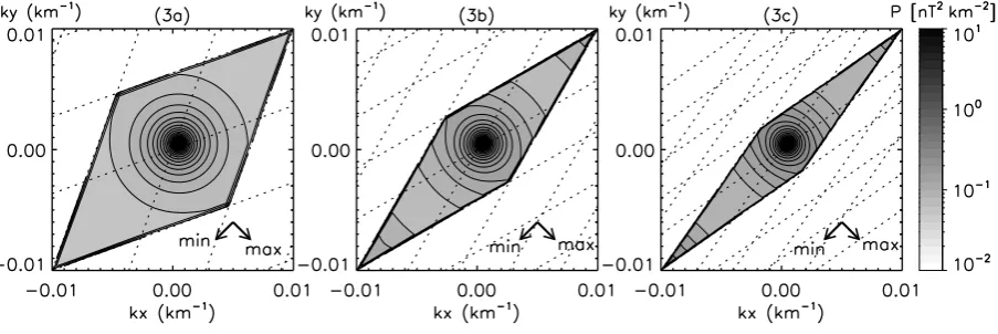
Case 3: Diamond-shaped cell

Reciprocal vectors are not always mutually orthogonal but have in general various angles. In such a case the Brillouin zone forms a diamond-shaped cell in the wave vector do-main. Figure 8 compares the Brillouin zones with three dif-ferent angles of the reciprocal vectors: 50◦ _{(3a), 30}◦ _(3b),

and 20◦_{(3c). Again, the true spectrum is the same as the}

Fig. 7. Aliased spectra for different rectangular cell shapes of the Brillouin zone, close to right square (left), moderately narrow in the vertical reciprocal vector length (middle), even narrower in that length (right). The dotted lines are parallel to the reciprocal vectors.

Fig. 8. Aliased spectra for different diamond-shaped Brillouin zones, with the angle between the two reciprocal vectors 50◦(left), 30◦ (middle), and 20◦(right).

isotropic except for the region near the corner of the Brillouin zone. The distribution is weakly elongated in the direction to the left-top and right-bottom corners which represents the shortest lattice vector direction, −k1+k2(toward the left-top corner of the cell) or−k1+k2(toward the right-bottom corner). Case (3b) exhibits the mutual angle 30◦ between the two reciprocal vectors, k1=(0.0127,0.0073)km−1 an k2=(0.0073,0.0127)km−1. The area of the isotropic distri-bution becomes smaller and the contour line are more aligned with the shortest lattice vector direction. Aliasing contribu-tion can also be found near the right-top and the left-bottom corners (in the direction to longest lattice vector directions, k1+k2) and the spectral energy increases near these cor-ners. Case (3c) exhibits even narrower angle, 20◦withk1= (0.0118,0.0082) km−1 and k2=(0.0082,0.0118) km−1. The isotropic distribution area is again small and the distribu-tion is overall anisotropic, though the elongadistribu-tion of the dis-tribution is not very much different from case (3b). At the right-top and the left-bottom corners the distribution exhibits

an enhanced contribution from the aliases such that the spec-tral energy first decreases and then increases near the corner of the cell in the longest lattice vector directions.

Case 4: Peak position in diamond-shaped cell

Fig. 9. Aliased spectra for different peak positions in a diamond-shaped Brillouin zone. The peak is shifted to the top side of the Brillouin

zone. Peak close to the origin in the cell (left), between the origin and the border of the cell (middle), and near the border (right).

Fig. 10. Enhancement parameter in the maximum (dotted lines) and the minimum distortion directions (solid lines) for the twelve spectra

presented in Figs. 6 to 9.

There is an asymmetry in the distribution between the right-top and left-bottom corners. The distorted distribution at the left-bottom corner comes from the alias(n1,n2)=(0,−1). In case (4c) this alias enters more in the Brillouin zone and two populations are identified in the distribution, the origi-nal peak at the top of the cell and its alias at the left-bottom corner. The distribution is isotropic near these peaks, oth-erwise the contour lines are elongated to the left-top corner direction.

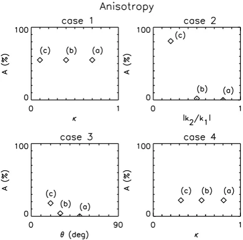
3.3 Quantitative analysis

The enhancement parameterE and the anisotropy parame-terAare determined for the twelve spectra (1a) to (4c) to

quantify the effect of aliasing. The enhancement parameter in each case is summarized in Table 2 at three distinct wave numbers from the spectral peak, and is also plotted in Fig. 10. Case 1

Table 2. Enhancement parameter for the twelve spectra in Figs. 6

to 9 in the maximum and the minimum distortion directions.

k (km−1) 0.002 0.004 0.006 case 1a max(E) 1.26 1.99 3.85

min(E) 1.25 1.77 2.49 1b max(E) 1.26 1.99 3.85 min(E) 1.25 1.77 2.49 1c max(E) 1.26 1.99 3.85 min(E) 1.25 1.77 2.49 case 2a max(E) 1.16 1.54 2.15 min(E) 1.16 1.53 2.06 2b max(E) 1.26 1.99 –

min(E) 1.25 1.77 2.49 2c max(E) 2.29 – –

min(E) 1.65 2.56 3.43 case 3a max(E) 1.24 1.82 2.74 min(E) 1.24 1.80 2.66 3b max(E) 1.43 – –

min(E) 1.38 2.18 3.35 3c max(E) 1.81 – –

min(E) 1.57 2.56 3.84 case 4a max(E) 1.43 – –

min(E) 1.38 2.18 3.35 4b max(E) 1.43 2.86 –

min(E) 1.38 2.18 3.35 4c max(E) 1.43 2.86 –

min(E) 1.38 2.18 3.35

in Fig. 11 (left top) as a function ofκ which is a relative closeness of the spectral peak to the boundary of the Bril-louin zone,

κ=

kc−kb kb

. (26)

Herekb denotes the boundary wave vector of the Brillouin zone closest from the spectral peakkc.

Case 2

In case (2a) the enhancement parameter almost degener-ates between the maximum and the minimum directions, and it increases from E=1.00 at the peak to E=2.15 (maximum) andE=2.06 (minimum) at the wave number 0.0060 km−1. Degenerated enhancement curves are a sign of almost isotropic distribution, and in fact the anisotropy parameter isA=4% at 0.0060 km−1. In case (2b) the max-imum enhancement increases fromE=1.00 at the spectral peak toE=2.7 at 0.0050 km−1. The largest wave num-ber in the maximum direction is diminished, reflecting the fact that the second reciprocal vectork2is shorter than that in case (2a). The minimum enhancement in (2b) increases from E=1.00 at the peak to E=2.49 at 0.0060 km−1. In case (2c) the wave number range for the maximum en-hancement is even shorter, and varies fromE=1.00 at the

Fig. 11. Anisotropy parameter as a function of the closenessκof the spectral peak to the boundary of the Brillouin zone measured at

k=0.0060 km−1from the spectral peak (case 1), the ratio of the two reciprocal vector magnitudes atk=0.0024 km−1(case 2), the angle between the two reciprocal vectors atk=0.0022 km−1(case 3), and the peak-boundary closenessκatk=0.0036 km−1(case 4).

peak toE=3.33 at 0.0024 km−1, whereas the minimum en-hancement varies from E=1.00 at the peak to E=1.84 at 0.0024 km−1 and to E=3.43 at 0.0060 km−1. The anisotropy parameter measured atk=0.0020 km−1isA= 0% (2a), 1% (2b), and 38% (2c). The anisotropy parame-ter increases more rapidly from (2a) to (2c) when measured at a larger wave number. Figure 11 displays the anisotropy parameter 4% (2a) to 29% (2b) and to 81% (2c) measured atk=0.0024 km−1(the maximum wave number available in case (2c)) as a function of the ratio of the two reciprocal vectors|k2/k1|. Anisotropy becomes stronger for a shorter second reciprocal vectork2.

Case 3

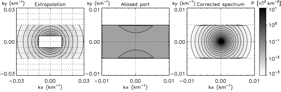
Fig. 12. Reconstruction of the spectrum by correcting the aliases. The spectrum is extrapolated for the neighboring cells in the wave vector domain (left panel), and then the alias of the extrapolated parts are estimated in the Brillouin zone (middle panel). The corrected or reconstructed spectrum is displayed in the right panel.

fromE=1.00 toE=1.57 at 0.0020 km−1. The anisotropy parameter increases moderately toward larger wave numbers in each case. For example, case (3a) exhibits the anisotropy parameter A=0%, 1%, and to 3% at k=0.0020 km−1, 0.0040 km−1, and 0.0060 km−1, respectively. Anisotropy in-creases a little more when the angle between the two recipro-cal vectors becomes narrower when measured at a fixed wave number. The anisotropy parameter is plotted as a function of the angle between the two reciprocal vectors in Fig. 11. Anisotropy increases for smaller angles of reciprocal vec-tors, and it varies from 0% (3a) to 4% (3b) and to 18% (3c) atk=0.0022 km−1(largest wave number available in (3c)). Case 4

Wave number range in the maximum enhancement direc-tion is short in (4a) and largest in (4c), but the three cases do not exhibit any significant difference in the enhance-ment parameter. The maximum enhanceenhance-ment parameter in-creases fromE=1.00 at the spectral peak to E=1.43 at k=0.0020 km−1in (4a), (4b), and (4c), and then toE=2.86 atk=0.0040 km−1in (4b) and (4c). The enhancement pa-rameter in the minimum direction increases fromE=1.00 at the peak to E=1.38 at k=0.0020 km−1, E=2.18 at k=0.0040 km−1, andE=3.35 atk=0.0060 km−1in (4a) to (4c). The anisotropy parameter isA=4% in the three cases when measured at=0.0020 km−1. Figure 11 plots the anisotropy parameter measured at =0.0036 km−1 (largest wave number available in (4a)) as a function ofκ, the close-ness of the spectral peak to the boundary of the Brillouin zone.

4 Correction of spatial aliasing

The procedure of correcting the spectrum for aliasing effect is mathematically to estimate in Eq. (9) or (23) the func-tionG for given functionP. There is, however, an uncer-tainty in this inverted-procedure because the true spectrum G must first be known to estimate the contribution of the aliases. The correction can in principle be achieved by an iteration scheme, that is to guess a true spectrum and then es-timate aliased spectrum using the reciprocal vectors and the assumed true spectrum. If the guessed spectrum yields an aliased spectrum which is close to the measured one, then the guessed spectrum can be used to correct the spectrum by subtracting the aliased part from the measured spectrum. If the guessed spectrum yields a different aliased spectrum from the measured one, then we modify the guessed spec-trum and repeat fitting procedure of the measured specspec-trum until the guessed spectrum provides a reasonably close spec-trum to the measurement.

middle). The measured spectrum is then finally corrected for the aliases (Fig. 12 right).

Our quantitative analysis suggests that anisotropy induced by spatial aliasing is small, say a few %, near the spec-tral peak under 20% of the longer reciprocal vector mag-nitude |k1|, except for a small ratio between the two re-ciprocal vectors|k2/k1|<0.5 or a small angle of the two vectors θ <30◦. Wave telescope technique developed for multi-spacecraft measurements (Pinc¸on and Lefeuvre, 1991; Motschmann et al., 1996; Glassmeier et al., 2001) provides the wave vector resolution better than 1% of the reciprocal vector (see Fig. 1 ranging over two orders of magnitude of wave number) and such a wave analysis technique is capa-ble of resolving the spectrum near its peak for correction of aliasing effect. Of course, there are always uncertainties in the correction procedure, in guessing the true spectrum, for example, if it is isotropic or anisotropic, or power-law or Gaussian curve, or to which order the aliases are taken into account (how many alias partners to be counted).

5 Conclusions

Aliasing is a general problem whenever discrete measure-ments sample continuous quantities. Periodic sampling of a continuous function results in a periodic structure in the Fourier domain. In this paper we have generalized alias-ing in the frequency domain to the wave vector domain, and shown that this spatial aliasing not only distorts the true spec-trum but also enters directly in the Brillouin zone. Aliasing in the wave vector domain has two effects, as investigated numerically in Sect. 3. One is weak aliasing, which yields anisotropy and asymmetry in the distribution. The distor-tion represents primarily elongadistor-tion of the distribudistor-tion in the shortest lattice vector direction. Weak aliasing is determined by the configuration of the reciprocal vectors and also by the peak position of the energy distribution in the Brillouin zone. Another effect is strong aliasing, in which the spectral en-ergy becomes dominated by the alias in some parts of the Brillouin zone. The distribution exhibits several peaks (orig-inal peak and aliased peak) in the case of strong aliasing. A possible method for correcting the spectrum for aliasing is also discussed. Using several assumptions the true spectrum can be recovered from the measured spectrum by estimating the aliasing contribution in the Brillouin zone. We conclude our study with a conjecture that if the correction method is applied to the wave telescope technique for real spacecraft data, spatial structures of the solar wind, the bow shock, and the magnetosphere will be more precisely determined. Acknowledgements. This work was financially supported by Bun-desministerium f¨ur Wirtschaft und Technologie and Deutsches Zen-trum f¨ur Luft- und Raumfahrt, Germany, under contract 50 OC 0901. Discussions with M. L. Goldstein and F. Sahraoui are grate-fully acknowledged.

Topical Editor I. A. Daglis thanks J. Vogt and another anony-mous referee for their help in evaluating this paper.

References

Angelopoulos, V.: The THEMIS Mission, Space Sci. Rev., 141, 5– 34, 2008.

Auster, H.-U., Glassmeier, K.-H., Magnes, W., Aydogar, O., Baumjohann, W., Constantinescu, D., Fischer, D., Fornac¸on, K.-H., Georgescu, E., Harvey, P., Hillenmaier, O., Kroth, R., Lud-lam, M., Narita, Y., Nakamura, R., Okrafka, K., Plaschke, F., Richter, I., Schwarzl, H., Stoll, B., Valavanoglou, A., and Wiede-mann, M.: The THEMIS Fluxgate Magnetometer, Space Sci. Rev., 141, 235–264, 2008.

Balogh, A., Carr, C. M., Acu˜na, M. H., Dunlop, M. W., Beek, T. J., Brown, P., Fornacon, H., Georgescu, E., Glassmeier, K.-H., Harris, J., Musmann, G., Oddy, T., and Schwingenschuh, K.: The Cluster Magnetic Field Investigation: overview of in-flight performance and initial results, Ann. Geophys., 19, 1207–1217, 2001, http://www.ann-geophys.net/19/1207/2001/.

Bracewell, B. J.: The Fourier Transform and its Applications, 3rd ed. McGraw-Hill, Boston, 2000.

Capon, J.: High Resolution Frequency-Wavenumber Spectrum Analysis, Proc. IEEE, 57, 1408–1418, 1969.

Chanteur, G.: Spatial interpolation for four spacecraft: Theory, in Analysis Methods for Multi-Spacecraft Data, G. Paschmann and P. Daly (eds.), ISSI Scientific Reports Series, ESA/ISSI, Vol. 1, pp. 349–370, 1998.

Escoubet, C. P., Fehringer, M., and Goldstein, M.: The Cluster mis-sion, Ann. Geophys., 19, 1197–1200, 2001,

http://www.ann-geophys.net/19/1197/2001/.

Glassmeier, K.-H., Motschmann, U., and Schmidt, R. (Eds.): Data Analysis Tools, Proc. CLUSTER Workshop, ESA-SP 371, Euro-pean Space Agency, Noordwijk, 1995.

Glassmeier, K.-H., Motschmann, U., Dunlop, M., Balogh, A., Acua, M. H., Carr, C., Musmann, G., Fornac¸on, K.-H., Schweda, K., Vogt, J., Georgescu, E., and Buchert, S.: Cluster as a wave telescope – first results from the fluxgate magnetometer, Ann. Geophys., 19, 1439–1447, 2001 (Correction, 21, 1071, 2003). Kirchner, J. W.: Aliasing in 1/fα noise spectra: Origins,

consequences, and remedies, Phys. Rev. E, 71, 066110, doi:10.1103/PhysRevE.71.066110, 2005.

Kittel, C.: Introduction to Solid State Physics, 7th ed., John Wiley & Sons, New York, 1996.

Motschmann, U., Woodward, T. I., Glassmeier, K.-H., Southwood, D. J., and Pinc¸on, J. L.: Wavelength and direction filtering by magnetic measurements at satellite arrays: generalized minimum variance analysis, J. Geophys. Res., 101, 4961–4965, 1996. Narita, Y., Glassmeier, K.-H., Sch¨afer, S., Motschmann, U., Sauer,

K., Dandouras, I., Fornac¸on, K.-H., Georgescu, E., and R`eme, H.: Dispersion analysis of ULF waves in the foreshock using cluster data and the wave telescope technique, Geophys. Res. Lett., 30, SSC 43–1, doi:10.1029/2003GL017432, 2003. Narita, Y. and K.-H. Glassmeier, Dispersion analysis of

low-frequency waves through the terrestrial bow shock, J. Geophys. Res., 110, A12215, doi:10.1029/2005JA011256, 2005.

terres-trial foreshock region, Phys. Rev. Lett., 97, 191101, doi:10.1103/PhysRevLett.97.191101, 2006.

Narita, Y., Glassmeier, K.-H., Frnz, M., Nariyuki, Y., and Hada, T.: Observations of linear and nonlinear processes in the foreshock wave evolution, Nonlin. Processes Geophys., 14, 361–371, 2007, http://www.nonlin-processes-geophys.net/14/361/2007/. Neubauer, F. and Glassmeier, K.-H.: Use of an array of satellites as

a wave telescope, J. Geophys. Res., 95, 19115–19122, 1990. Nyquist, H.: Certain topics in telegraph transmission theory, Amer.

Inst. Elect. Eng., 47, 617–644, 1928.

Paschmann, G. and Daly, P. W. (Eds.): Analysis Methods for Multi-Spacecraft Data, ISSI Scientific Report, SR-001, ESA Publica-tions Division, Noordwijk, The Netherlands, 1998.

Paschmann, G. and Daly, P. W. (Eds.): Multi-Spacecraft Analysis Methods Revisited, ISSI Scientific Report, SR-008, ESA Com-munications, Noordwijk, The Netherlands, 2008.

Pinc¸on, J. L. and Lefeuvre, F.: Local characterization of homoge-neous turbulence in a space plasma from simultahomoge-neous measure-ment of field components at several points in space, J. Geophys. Res., 96, 1789–1802, 1991.

Sahraoui, F.; Pinc¸on, J. L., Belmont, G., Rezeau, L., Cornilleau-Wehrlin, N., Robert, P., Mellul, L., Bosqued, J. M., Balogh, A., Canu, P., and Chanteur, G.: ULF wave identifica-tion in the magnetosheath: The k-filtering technique applied to Cluster II data J. Geophys. Res., 108, SMP1-1, 1335, doi:10.1029/2002JA009587, 2003.

Sahraoui, F., Belmont, G., Rezeau, L., Cornilleau-Wehrlin, N., Pinc¸on, J. L., and Balogh, A.: Anisotropic tur-bulent spectra in the terrestrial magnetosheath as seen by the Cluster spacecraft, Phys. Rev. Lett., 96, 075002, doi:10.1103/PhysRevLett.96.075002, 2006.

Shannon, C. E.: Communication in the presence of noise, Proc. IRE, 37, 10–21, 1949.

Tjulin, A., Pinc¸on, J.-L., Sahraoui, F., Andr´e M., and Cornilleau-Wehrlin, N.: The k-filtering technique applied to wave electric and magnetic field measurements from the Cluster satellites, J. Geophys. Res., 110, A11224, doi:10.1029/2005JA011125, 2005. Unser, M.: Sampling – 50 years after Shannon, Proc. IEEE., 88,

569–587, 2000.

Vogt, J., Narita, Y., and Constantinescu, O. D.: The wave surveyor technique for fast plasma wave detection in multi-spacecraft data, Ann. Geophys., 26, 1699–1710, 2008,