Non-spherical source-surface model of the heliosphere: a scalar formulation

Non-spherical source-surface model of the heliosphere:

a scalar formulation

M. Schulz

Space Sciences Department, Lockheed Martin Palo Alto Research Laboratories, 3251 Hanover Street, Palo Alto, California 94304 (USA)

Received: 19 September 1995 / Revised: 24 October 1996 / Accepted: 30 October 1996

Abstract. The source-surface method offers an

alter-native to full MHD simulation of the heliosphere. It entails specification of a surface from which the solar wind flows normally outward along straight lines. Compatibility with MHD results requires this (source) surface to be non-spherical in general and prolate (aligned with the solar dipole axis) in prototypical axisymmetric cases. Mid-latitude features on the source surface thus map to significantly lower latitudes in the heliosphere. The model is usually implemented by deriving the B field (in the region surrounded by the source surface) from a scalar potential formally ex-panded in spherical harmonics, with coefficients chosen so as to minimize the mean-square tangential compo-nent of B over this surface. In the simplified (scalar) version the quantity minimized is instead the variance of the scalar potential over the source surface. The scalar formulation greatly reduces the time required to compute required matrix elements, while imposing essentially the same physical boundary condition as the vector formulation (viz., that the coronal magnetic field be, as nearly as possible, normal to the source surface for continuity with the heliosphere). The source surface proposed for actual application is a surface of constant F~rÿk_{B, where}~ _{r is the heliocentric distance}

and~Bis the scalar magnitude of the B field produced by currents inside the Sun. Comparison with MHD simulations suggests that k1:4 is a good choice for the adjustable exponent. This value has been shown to map the neutral line on the source surface during Carrington Rotation 1869 (May–June 1993) to a range of latitudes that would have just grazed the position of Ulysses during that month in which sector structure disappeared from Ulysses’ magnetometer observations.

1 Background

The magnetic field in the solar corona is traditionally modeled (Schatten et al., 1969; Altschuler and Newkirk, 1969; Hoeksema and Scherrer, 1986; Hoeksema, 1991) as being current-free (and thus derivable from a scalar potential) within a spherically annular volume of inner radius 1r and outer radius r0 1:6ÿ2:5r sur-rounding the Sun. The inner sphere …rˆr†

corre-sponds to the photosphere, at which the line-of-sight component of the Sun’s magnetic field B is remotely observed by means of Earth-based Zeeman spectros-copy. The outer sphere …rˆr0† is regarded as a magnetic equipotential surface, to which B is therefore perpendicular and from which the solar wind implicitly flows radially outward into the heliosphere. Schatten

et al. (1969) chose r0ˆ1:6r for the radius of their source surface. Altschuler and Newkirk (1969) chose r0 ˆ2:5r in order to achieve better agreement with dimensions of large coronal helmet structures seen in eclipse photographs.

Hoeksema (1995) currently use a modified version of Schatten’s approach, treating these two radii as adjus-table parameters of their model (see also Wang and Sheeley, 1995).

In a lesser known alternative formulation, Schulz

et al. (1978) gave the source surface of Altschuler and

Newkirk (1969) a non-spherical shape (still enclosing a volume 125pr3=6) but preserved its role as a magnetic equipotential surface from which the solar wind flows normally outward along straight lines. The particular shape of source surface chosen by Schulz et al. (1978) to illustrate the new model was an isogauss of the Sun’s dipole field. The equation of this source surface (of equatorial radiusr0 2:3r) wasrˆ …1‡3 cos2h†1=6r0, where hdenotes the magnetic colatitude. The essential feature of this surface was its prolateness along the dipole axis.

Schulz et al. (1978) found that rectilinear trajectories extending normally outward from such a source surface adequately simulated the field-line directions obtained by Pneuman and Kopp (1971a, b) from their MHD solution (see Fig. 1b) and adequately spread magnetic field lines throughout the heliosphere, so that the meridional ( radial) component of B was virtually independent of magnetic latitude at any specified rJ1 AU. Ulysses observations by Smith and Balogh (1995) have confirmed this (the latitude-independence of r2_B

r)

as a desirable result.

Levine et al. (1982) applied the concept of Schulz

et al. (1978) to a more realistic (not purely dipolar)

heliomagnetic field. The magnetic field Bˆ ~B‡ B in the

region rrrs…h; u) between the photosphere and

the non-spherical source surface was again separated into contributions due to currents at r<r and at

rrs…h;u), respectively, so that

~

Bˆ ÿrr

XN

nˆ1 Xn

mˆ0

…r=r†n‡1‰gmn cosmu‡h m

n sinmuŠP m n…h†

…1a†

Bˆ ÿ…r3=r₀2†rX

N

nˆ1 Xn

mˆ0

…r=r0†n‰gmn cosmu

‡ hmn sinmuŠP m

n…h† …1b†

wherer0is a nominal (e.g., equatorial) radius character-izing the source surface and thus normalcharacter-izing the expansion coefficients gm

n; hmn

8 9

in Eq. (1b). The expansion coefficients gmn; h

m n

8 9

in the work of Levine et al. (1982) were obtained by minimizing (with respect to the gm

n; h m n

8 9

) a bilinear variational quantity equal to the mean-square tangential component of B over the source surface. (The goal of this procedure was to make B as nearly as possible normal to the source surface from the inside.) The value ofrˆrs…h; u†on the source surface was implicitly specified by adopting a compromise between a source surface of constantB~2_(as in Schulz et al., 1978) and a source surface of constantr (as in Altschuler and Newkirk, 1969). The present work offers a simplified prescription of the source surface and a streamlined determination of the coefficients gm

n; h m n

8 9

,

in the hope that these steps will make the model easier to use in practice.

2 Source surface

The source surface in the present work is regarded (Schulz, 1995) as a surface of constantF~rÿk_{B, where}~

~

B…j ~Bj) is the absolute value of the magnetic field B~

produced by currents inside the Sun and k…0† is an

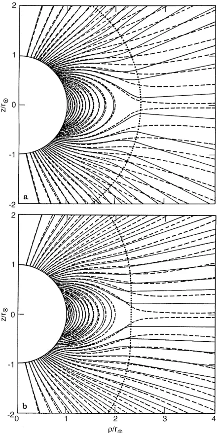
Fig. 1a,b. Representative field lines emanating from selected

photo-spheric latitudes in various coronal magnetic-field models, applied to the case in which the Sun’s field is dipolar. Dashed curves correspond to MHD model of Pneuman and Kopp (1971a,b) in both panels. Solid curves correspond to source-surface models: a with spherical source surface (dotted curve) of radius rˆ2:5r (Altschuler and Newkirk, 1969), corresponding tokˆ 1in present notation; and b with ‘‘dipole-isogauss’’ source surface (dotted curve) of variable radius

rˆ2:3…1‡3 cos2_†1=6_r

adjustable parameter. The limitk! 1leads back to the usual spherical source surface (Schatten et al., 1969; Altschuler and Newkirk, 1969), which was intended primarily for modeling the corona (not the entire heliosphere). The choice kˆ0 leads back to a source surface of constant B~ (Schulz et al., 1978). For the special (test) case of a dipolarB field (but for general~ k) the equation of a source surface with equatorial radius r0 would be

rˆ …1‡3 cos2h†1=…2k‡6†r0; …2† where h is the magnetic colatitude. The unit vector ^n

normal to the source surface would be given in spherical coordinates by

^

n ÿ j r~F jÿ1 r~F

ˆ 3^hcoshsinh‡ …k‡3†^r…1‡3 cos2h† ‰9 cos2_hsin2_h‡

k‡3†2…1‡3 cos2_h†2_Š1=2 : …3† The direction of ^n is easier to visualize in cylindrical

coordinates (qrsinh; zrcosh), since the value of dz

dqˆ

‰k‡3…k‡4†cos2_hŠcosh

‰…k‡3† ‡3…k‡4†cos2_hŠsinh …4† along ^n at the source surface is equal to the tangent of

the heliomagnetic latitudekto which the corresponding field line would map asymptotically. This dz=dqshould well approximate the value of tankalong the field line at r1:1ÿ5:4 AU (the range spanned by Ulysses). However, the actual equation of a solar-wind stream-line, from the source surface to the boundary of the heliosphere in this model, is

zˆzs‡ …dz=dq†s…qÿqs†; …5† where the subscript s denotes evaluation at the source surface (Schulz et al., 1978).

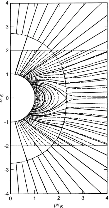
The dotted curve in Fig. 2 corresponds to the source surface specified by Eq. (2) forkˆ1:4, withr0chosen so as to preserve the enclosed volume…ˆ125pr3

=6†. In this

case a source surface of equatorial radius r02:33r would enclose the same volume as a sphere of radius 2:5r. The solid lines in Fig. 2 extend normally outward from selected latitudes (5 apart) on the source surface, for comparison with the directions of MHD field lines (dashed curves) obtained by Pneuman and Kopp (1971a, b). This comparison confirms that k1:4 is a reasonable choice for the shape parameter k in Eq. (2), at least for the dipolar test case. Moreover, the choice of kˆ1:4 has been found (Schulz, 1995) to account within 1 for the maximum latitude (30S) reached by the heliospheric current sheet (HCS) at r4:7 AU during May 1993, when ‘‘sector structure’’ first disappeared from the Ulysses magnetometer observations (Smith

et al., 1993).

Since the Sun’s B field is predominantly dipolar only during part of the solar cycle, extending for a few years on either side of solar minimum, it may be premature to infer that the same choice for k should apply under solar-maximum conditions also. For now this is just a working hypothesis to be tested against future Ulysses

data. However, Levine et al. (1982) found that a similarly (although parametrically more cumbersome) intermediate shape between kˆ0 and kˆ 1 could account quite well not only for the MHD field configuration obtained by Pneuman and Kopp (1971a,b) in the dipolar test case, but also for a more complicated coronal and interplanetary B-field config-uration encountered not far from solar maximum.

3 Variational principle

The magnetic field B (ˆ ~B‡B ) specified by Eq. (1) is

derivable from a scalar potentialV…ˆ ~V ‡V†atrr0. The vector B is made everywhere perpendicular to the spherical source surface (of radius r0) employed in the model of Schatten et al. (1969) or Altschuler and Newkirk (1969) by choosing the expansion coefficients

Fig. 2. Dashed curves represent field lines emanating from selected

photospheric latitudes in MHD model of Pneuman and Kopp (1971a, b) for the case in which the Sun’s field is dipolar. Solid curves represent field lines that cross the source surface, specified as

rˆ2:33…1‡3 cos2_h†5=44

fgm n;h

m

ng in Eq. (1b) so that …g m n;h

m n† ˆ …g

m n;h

m n†. This

choice offgm n;h

m

ngmakes the source surface (rˆr0) an equipotential ofV. Indeed, it makesV ˆ0 (regardless of

handu) atrˆr0.

The magnetic field Bˆ ÿrV specified by Eq. (1) is made (as nearly as possible) perpendicular to a prolate source surface in the model of Schulz et al. (1978) and Levine et al. (1982) by minimizing the variational quantity

r I

ss

…n2B†2dA …6†

with respect to the expansion coefficientsfgm n;h

m

ngin Eq.

(1b). This procedure seems simple enough in concept, but its implementation in general has led to page-long equations and correspondingly long computation times (Levine et al., 1982).

The present work offers a simpler procedure for making B (as nearly as possible) normal to the source surface from the inside. The variational quantity minimized here is

r3 I

ss

…V ÿ hVi†2dA; …7†

wherehVidenotes the mean value ofV over the source surface. (It is easy to show that, if the goal is to minimize the mean-square deviation ofV from a constant over the source surface, then that constant must behVi). As long as B is to be derived from a scalar potential in the region surrounded by the source surface, a scalar formulation based on Eq. (7) seems simpler to implement than a vector formulation based on Eq. (6). The results should be equivalent, if not identical.

The coefficientsfgmn;h m

ngare presumed to have been

determined (e.g., Hoeksema and Scherrer, 1986) from the line-of-sight component of B, as measured through Earth-based Zeeman spectroscopy. That deconvolution typically invokes a spherical source surface of radius rˆ2:5r. Better values for the coefficients fgmn;h

m ng

could possibly be deduced through use of a prolate source surface, but this potential refinement (which would seem to require an iterative deconvolution of the solar magnetic-field data) is not addressed here. Only the coefficients fgmn;h

m

ng are evaluated via Eq. (7) in the

present work.

Since r3 is algebraically bilinear in the expansion coefficientsfgmn;h

m

ng, the equations dr3=dgm

0

n0 ˆdr3=dhm

0

n0

ˆ0 suffice to determine optimal values for the N…N‡2† coefficientsfgmn;h

m

ng. There are…N=2†…N‡3†linear

equa-tions of the form

or3 ogm0 n0

ˆ2 I

ss

…V ÿ hVi† oV

ogm0 n0

ÿohVi

ogm0 n0 dA ˆ2 I ss

…V ÿ hVi†‰oV=gm_n00ŠdAˆ0; …8a†

corresponding to distinct values of (n0;m0), and …N=2†…N‡1† linear equations of the complementary form

or3 ohmn00

ˆ2 I

ss

…V ÿ hVi† oV

ohmn00

ÿohVi

ohmn00

" #

dA

ˆ2 I

ss

…V ÿ hVi†‰oV=ohmn00ŠdAˆ0; …8b†

also corresponding to distinct values of (n0;m0). The parenthesized factor in Eq. (8) is linear with respect to thefgmn;h

m

ngin each case; the factors in square brackets

can depend on (n0;m0) but not explicitly on fgmn00;h m0 n0g,

since V itself depends linearly on fgm0 n0;h

m0

n0g in that

factor. The terms ohVi=ognm00 and ohVi=oh m0

n0 can be

removed from the square-bracketed factors in Eqs. (8a) and (8b), respectively, because they are independent of spatial coordinates. Thus, they behave as constants in any integrations over the source surface of whatever shape, which thus reduce to integrals of…V ÿ hVi†with respect to dA over the source surface. Such integrals vanish by definition:hViis the mean value ofV over the source surface. A further simplification (such that hVi ˆ0) occurs if B (and thus the source surface itself)~

is adequately symmetric between north and south. Otherwise it is necessary to implement Eqs. (8a) and (8b) as they stand, accepting that hVi can depend on fgm0

n ;h m0

n gifhVi 60. 4 Test case

The greatly simplified case of dipolar B illustrates how~

this described variational procedure might work in practice. The source surface in this case reduces to that specified by Eq. (2), and the magnetic field B given by Eq. (1) becomes derivable from the scalar potential V…r;h† ˆg01…r3=r2†cosh

‡ …r3=r20†X

N

nˆ1

…r=r0†ng0nPn…cosh†; …9†

with only odd values of n…ˆ1;3;5; :::† represented in the summation. Legendre functions

Pn…x† ˆ

1 n!2n

dn dxn

2

…x2ÿ1†n3 …10a†

satisfy the differential equation d

dx 2

…1ÿx2†dPn dx

3

‡n…n‡1†Pn…x† ˆ0: …10b†

It follows from Eq. (9) that dV=dg0

n0 ˆ …r3=r20†2

…r=r0†n0Pn0…x†, where xˆcoshP1…x†. Thus, it follows

from Eq. (8a) that XN

n_ˆ1 g0n

I

ss

…r=r0†n‡n0Pn…x†Pn0…x†dA

ˆ ÿg0₁ I

ss

…r=r0†n0ÿ2xPn0…x†dA …11a†

dAˆ4pr2 1‡ 3x

2_1ÿx2_† …k‡3†2…1‡3x2†2

" #1=2

dx …11b†

for 0x1. The required integrals have been evaluated numerically with Mathematica (Wolfram, 1992), which has also been programmed to solve the resulting simultaneous linear equations specified by Eq. (11). Results for fg0n=g01g corresponding to selected

values of N…ˆ3;5;7; :::;15† are listed in Table 1. Truncation of Eq. (1b) at ˆ1 would be contrary to the spirit of the model but is found to yield g0n=g01ˆ ÿ0:708580.

The values of g0n=g01 in Table 1 represent normalized 2n_{-pole moments due to azimuthal currents that flow}

outside the source surface. These values specify the relative weights that should be assigned to the various P0_n…h†in Eq. (1b) if the Sun’s own magnetic field (B) were~

purely dipolar. The value ofg0n=g01in any row of Table 1 seems to approach a limit asN ! 1, but the values of fg0n=g01g in any column of Table 1 are mutually

optimized for the corresponding N. Strictly speaking, this means that Eq. (1b) is not a uniformly convergent representation of B unless kˆ 1(i.e., unless the source surface is spherical). One cannot just truncate any column in Table 1 at some n<N and expect the resulting representation to be ‘‘good enough.’’ Even so, there is little visible difference between theN ˆ13 model and the N ˆ11 or theN ˆ15 model when representa-tive field lines are plotted for comparison with Pneuman and Kopp (1971a, b).

Magnetic field lines in heliospheric models are usually traced numerically (e.g., by using a fourth-order Runge-Kutta technique) as space curves locally tangential to B. However, the tracing procedure can be greatly simpli-fied, at least for an axisymmetric B field derived from a scalar potential, by formally constructing Euler poten-tials …a;b† such that bˆu and Bˆ ra2 rbˆ ÿrV (e.g., Stern, 1976, 1994)

1 rsinh

^r

r

oa

ohÿ ^hooar

ˆ ^roV or ‡

^

h

r

oV

oh …12†

This means that

oa=ohˆ ÿr2sinh…oV=or† …13a† and that

oa=orˆsinh…oV=oh† …13b†

for the case of a current-free axisymmetric B field. (This is admittedly a very special test case, unlikely to be encountered in nature.) Thus, it follows from Eq. (13a) that

a…r;h† ˆg01…r3=r†…1ÿx2† ‡ …r3=r0†X

N

n_ˆ1

…r=r0†n‡1g0_n …nÿ1†!2n

dnÿ1 dxnÿ1 ‰…x

2_ÿ1†n

Š …14a†

and from Eq. (13b) that

a…r;h† ˆg01…r3=r†…1ÿx2† ÿ …r3=r0†…1ÿx2†X

N

nˆ1

…r=r0†n‡1g0n

…n‡1†!2n

dn‡1 dxn_‡1 2

…x2ÿ1†n3: …14b†

That these two expressions fora…r;h†are equivalent can be seen by integrating Eq. (10b) with respect to x. The latter form of Eq. (14) is probably the more convenient, however: This form shows sin2h…ˆ1ÿx2_{†explicitly as a} factor common to all terms in the summation, leaving the derivative (rather than the integral) of Pn…x† with

respect to x to be generated (as a callable function) by Mathematica (Wolfram, 1992).

The value ofaat any point along a field line must be equal to 1=2p times the magnetic flux enclosed by rotating that field line about the symmetry axis. That a andbremain constant along any field line is well known and obvious, since ra1 …ra2 rb† ˆ rb1 …ra2 rb† ˆ0. (The cross product between any two vectors is always perpendicular to each.) Thus, it follows from Eq. (14b) that the quantity

1

Lˆ …1ÿx 2_†

r=r† 1ÿX

N

nˆ1

…r=r0†n‡2…g0

n=g01†

…n‡1†

dPn

dx

" #

…15†

should remain constant on the magnetic surface (shell of field lines) that it labels. (The ‘‘L’’ terminology is borrowed from magnetospheric physics. The idea is that a dipolar field line would satisfy the equation rˆLrsin2h and so would intersect the photosphere

at a magnetic latitude K such that cosKˆLÿ1=2_{.) In a} field geometry stretched by the heliospheric current sheet, the enclosed magnetic flux remains proportional to 1=L, but the field line intersects the equator atr>Lr

and the photosphere at a magnetic latitude slightly higher than cosÿ1_Lÿ1=2_{†. Thus, for example, the last}

Table 1. Optimized values ofg0_n=g0₁for selected values ofN

n Nˆ3 Nˆ5 Nˆ7 Nˆ9 Nˆ11 Nˆ13 Nˆ15

1 )0.723974 )0.725645 )0.725908 )0.725957 )0.725967 )0.725970 )0.725970

3 +0.0941047 +0.103736 +0.105261 +0.105550 +0.105610 +0.105624 +0.105627

5 0.0 )0.0274149 )0.0324136 )0.0334301 )0.0336532 )0.0337049 )0.0337174

7 0.0 0.0 +0.00944986 +0.0119309 +0.0125432 +0.0126956 +0.0127342

9 0.0 0.0 0.0 )0.00351930 )0.00472703 )0.00507664 )0.00517369

11 0.0 0.0 0.0 0.0 +0.00137132 +0.00195296 +0.00214590

12 0.0 0.0 0.0 0.0 0.0 )0.000550607 )0.000828866

closed field line (which reaches xcoshˆ0 at rˆr0 ˆ2:33r) in the present model bears the label L3 ˆ1:6425 and crosses the photosphere at magnetic latitude K3ˆ39:69. A purely dipolar field line with Lˆ1:6425 would cross the photosphere at Kˆ38:71. For a spherical source surface of radius rˆ2:5r, the last closed field line would have borne the labelL3ˆ5=3 and would have intersected the photosphere at

K3_{ˆ40:32. These differences are not major. Moreover,}

the present source-surface model (withkˆ1:4) and the model with a spherical source surface (kˆ 1) differ only slightly with respect to the field-line configuration atrK0:8r0: Decisive differences in field-line configura-tion appear only in the outer part of the region enclosed by the source surface and (especially) in the mapping of field lines from the source surface into the heliosphere.

The solid curves in Fig. 2 are selected field lines constructed via Eq. (15) from the values ofg0n=g01 shown in Table 1 forNˆ15. These field lines have been chosen so as to intersect the source surface at 15 intervals of magnetic latitude. The superposed dashed curves are field lines from the MHD simulation of Pneuman and Kopp (1971a, b), as in Fig. 1. These had been chosen so as to intersect the photosphere at a convenient set of latitudes (not evenly spaced). Thus, the dashed and solid curves in Fig. 2 do not correspond one-to-one. The noteworthy feature is their ‘‘nested’’ relationship: They tend to interleave rather than intersect.

5 Heliospheric field intensity

The amount of magnetic flux poleward of the magnetic shell that bears the label a…ˆg0

1r2=L† is equal to 2pa, and so the mean value of jBrj over any heliocentric

sphere of radius rr0 must be equal to jg0₁r2=r2L3j. Since L3 ˆ1:6425 (see earlier), this means that h…r=AU†2jBrji 1:317210ÿ5jg01j if r=AU is the

helio-centric distance measured in AU…1AU215r†: The latitudinal distribution of this field intensity is of interest here for comparison with Ulysses results.

Since the construction of field lines outside the source surface is essentially geometrical, it is easy to calculate the corresponding field intensity geometrically (by invoking magnetic flux conservation). The solid straight lines in Fig. 2 are normal to the source surface, and each can be considered to radiate from a center of curvature in the same meridional plane (Schulz et al., 1978, Fig. 4). The radius of curvature of a magnetic meridian on the source surface is given by

which reduces to rcˆ …k‡3†…r0=k† ˆ …22=7†r0 at the

equator …hsˆp=2† and to rcˆ4‰…k‡3†=…4k‡15†Š2

21=…k_‡3†_{r0ˆ1:000141r0 at the poles …h}

sˆ0;p) if kˆ7=5. The value of Br along either polar field line

(beyond the source surface) thus varies as

Brˆ 60:135693g01‰2:330329r=…rÿ0:397215r†Š2 …17†

since the surrounding field lines would fill an infinitesi-mal cone with its apex at zˆ 6‰3=…4k‡15†Š21=…k‡3†_r0 along the axis of symmetry (see Schulz et al., 1978).

The geometry is a bit more complicated for mappings from other latitudes on the source surface, but the principle is the same: The meridional component of B should vary as the ratio between corresponding infini-tesimal areas (transverse to the solar-wind velocity) on the source surface and (as mapped to the point of interest) in the heliosphere. The ratio of such areas can be expressed (Schulz et al., 1978) as

Bm

Bs ˆ

rcqs

frc‡ ‰…qÿqs†

2_‡

zÿzs†2Š1=2gq

ˆ rcqs

frc‡ …qÿqs†‰1‡ …dz=dq†

2

sŠ

1=2

gq; …18†

where…q;z†are the cylindrical coordinates of the point of interest in the heliosphere and…qs;zs†are the cylindrical

coordinates of the corresponding point on the source surface. The linear mapping of a field line from…qs;zs†to

…q;z†is specified by Eq. (5). The meridional component of B (calledBmin the heliosphere and Bs on the source

surface) is simultaneously equal to …B2

r‡B2h†

1=2 and …B2

q‡B2z†

1=2

. This differs only very slightly from Br,

however, at heliocentric distancesrJ1 AU…rc†.

It seems most convenient to map from a selected point …qs;zs† on the source surface to a chosen

heliocentric distance r in the heliosphere. The corre-sponding value of…qÿqs†, which is needed in Eq. (18),

can be obtained by solving the quadratic equation r2ˆ …qÿqs‡qs†

2

‡ …zÿzs‡zs†2

ˆ ‰1‡ …dz=dq†2_sŠ…qÿqs†

2 ‡r2s

‡2‰qs‡zs…dz=dq†sŠ…qÿqs†; …19a†

where r2

s q2s‡z2s. The solution forqqs is

‰1‡ …dz=dq†2_sŠ…qÿq_s† ˆ f‰qs‡zs…dz=dq†sŠ

2

‡ ‰1‡ …dz=dq†2_sŠ…r2ÿr2_s†g1=2

ÿ ‰qs‡zs…dz=dq†sŠ …19b†

The colatitudehof the heliospheric point to which…qs;zs†

maps is indicated by Eq. (5). It is not practical to select the heliospheric point …q;z†first and then map back to the source surface, since the value of…dz=dq†_sneeded for

making this mapping is dependent on…qs;zs†and would

thus remain unknown until the mapping was completed. The limitr!1yields…qÿqs†q!‰1‡ …dz=dq†

2

sŠÿ

1 r2 and ctn h! …dz=dq†_s. The asymptotic value of …r=r†2Bm is thus given by

rcˆ …

1‡3 cos2_hs†ÿ…2k‡5†=…2k‡6†_{r0‰…1‡3 cos}2_hs†2

…k‡3†2‡9 cos2_h

ssin2hsŠ3=2 …k‡3†‰…1‡3 cos2hs†2…_k‡₃†2‡_{9 cos}2h

ssin2hs‡3…k‡3†…5 cos2hsÿ1†Š

…r=r†2Bm! …rcqs=r2†‰1‡ …dz=dq†

2

sŠ

1=2

Bs: …20†

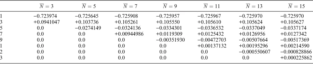
This quantity is plotted (solid curve) in Fig. 3, but as a function of the heliomagnetic latitude k90ÿh. The latitude k along a field line specified by Eq. (5) approaches tanÿ1…dz=dq†_s as r! 1. As would be expected, the asymptotic plot of…r=r†2Bm againstkin

Fig. 3 is almost indistinguishable from a plot of …r=r†2Bm against k at rˆ1 AU (not shown). The

meridional (asymptotically radial) component of B in this model varies by about 618% from its mean value over about 80% of the unit sphere. A source-surface model with kˆ1:4 thus leads (not surprisingly) to a latitudinal distribution of magnetic flux similar to that found by Pneuman and Kopp (1971a, b).

The dashed step-function in Fig. 3 corresponds to a hypothetically uniform latitudinal distribution of the same amount of magnetic flux, which would be in better agreement with the Ulysses observations (Smith and Balogh, 1995). The meridional component of B atrˆ1 AU actually is almost latitude-independent (varying by less than65% from its mean value over 85% of the unit sphere) in a source surface model with kˆ0 (Schulz

et al., 1978), which corresponds to Fig. 1b here. A

spherical source surface (kˆ 1, corresponding to Fig. 1a here) would have led to a sinusoidal variation of Br with latitude: Br ˆ3g01…r3=r2r0)sink, which is

contrary to all observations.

6 Summary and discussion

If the criterion for a successful heliospheric model were just that …r=r†2Bm be almost independent of kat rK1

AU, there might be reason to prefer the kˆ0 source

surface (Schulz et al., 1978) over the present kˆ1:4 version. However, a comparison between Figs. 2 and 1b confirms that the present version better accounts for the latitude-dependent direction of B outside the source surface, and Schulz (1995) found that thekˆ1:4 model accounts better (almost perfectly, in fact) for the Ulysses-inferred latitudinal extent (Smith et al., 1993) of the heliospheric current sheet (HCS) during Carring-ton Rotation 1869 (May–June 1993, when sector structure first disappeared from Ulysses’ magnetometer observations).

It seems that only a slightly equatorward redistribu-tion of the normal component of B over the present (kˆ1:4) source surface could preserve the desired directionality and mapping properties achieved here, while also restoring the near-uniformity of …r=r†2Bm

with magnetic latitude previously achieved with the kˆ0 model. Uniqueness of solutions to Laplace’s equation for the Dirichlet problem (e.g., Jackson, 1962) posed here [and solved via Eq. (7)] precludes such a redistribution of ^n1B within the framework of

potential theory. Thus, further improvements in model-ing the heliosphere by source-surface methods would seem to require that currents be permitted to flow inside the region surrounded by the source surface. This is not a radical requirement, of course: it seems quite reason-able that the corona would contain plasma currents that merge smoothly into the HCS. A source-surface model that precludes such currents is just too naive in the present context.

The dual source-surface model of Schatten (1971) already provides for a current-bearing coronal transition region (1:6rKrK2:5r) and thus partially answers the foregoing objection. Another interesting approach, however, would be to add currents implicitly through a

B-field expansion not based on spherical harmonics

(e.g., Schulz and Eviatar, 1969; Mead and Fairfield, 1975). This approach would, of course, require that Eq. (7) be abandoned in favor of Eq. (6), as a means of enforcing (in the least-squares sense) the usual boundary condition that calls for the tangential component of B preferably to vanish everywhere on the source surface. In other words, the present (scalar) formulation of the heliospheric source-surface model can apply only if the magnetic field B is derivable from a scalar potentialV in the region enclosed by the source surface. If the region surrounded by the source surface were permitted to contain implicit currents, then the assumed volume of this region might reasonably be enlarged so as not to increase the overall amount of open magnetic flux. This step might help bring the solid curves in Fig. 2 into better agreement with the MHD field lines (dashed curves), which do remain significantly curved well beyond the present source surface (dotted curve). (An increase of 20–25% in source-surface volume would, for example, increase the equatorial radius r0 in Eq. (2) from 2:33r to 2:5r).

There are several levels of sophistication at which a non-spherical source surface can be used for helio-spheric modeling. The trade-off is between realism and convenience. As has been noted here, the required

Fig. 3. Variation of meridional (asymptotically radial) component of

(r=r†2B[component denoted (r=r†2Bm] with heliomagnetic latitude

k…90ÿh) in the limit r! 1, in a source-surface model with

kˆ7=5 for the case in which the Sun’s field is dipolar. For comparison (dashed step-function): hypothetical case (quite well approximated (Schulz et al., 1978) by a source-surface model with

algebra and numerical computations can be simplified by adopting a scalar formulation of the variational problem, minimizing Eq. (7) instead of Eq. (6) with respect to the expansion coefficients for B. However, a scalar formulation requires us to assume (as usual) that the region enclosed by the source surface is current-free, whereas comparisons of model results with various Ulysses observations cast serious doubt on this assump-tion. (The modeling of twisted coronal loops has long required field-aligned currents in the same region of space, but it has been hoped that such currents would be of sufficiently small scale not to influence heliospheric mappings.)

Another possible simplification is to use Eq. (2), rather than a surface of truly constantF~ˆrÿkB, as the~ postulated source surface, even when B is not purely~

dipolar (as it never is in reality). This was the simplifying approach used by Schulz (1995) in a seemingly success-ful mapping of the neutral line on the source surface (see Hoeksema, 1991) to a range of heliospheric latitudes just grazed by Ulysses during Carrington Rotation 1869 (May-June 1993). If such a model source surface is Sun-centered and aligned with the heliomagnetic dipole axis, then Eqs. (7) and (8) are automatically simplified through the fact that hVi 0 by symmetry. [It would be possible with any source-surface geometry to make hVi ˆ0 by adding an appropriate constant to an expression such as Eq. (9), but the appropriate constant would then typically depend on the fgmn;h

m

ng. Only

symmetry, such that the mean value of each spherical-harmonic function over the source surface is zero, can remove the attendant complication of Eq. (8) by making hVi 0 without such an additive constant, regardless of what values are assigned to thefgmn;h

m ng.]

However, the use of Eq. (2) as a simplified source surface regardless of the form of B seems likely to be~

successful only near solar minimum, when B is in fact~

most nearly dipolar. The goal in choosing a non-spherical source surface is to arrange for the region(s) of minimal source-surface curvature to straddle the inner edge(s) of any heliospheric current sheet(s). The choice of a surface of constantF~ as source surface shows some promise in this regard (Schulz et al., 1978; Levine et al., 1982; and in the present work) but is not guaranteed to achieve the desired configuration. However, the purpose is likely to be defeated altogether (especially near solar maximum, when B is quite complicated and multiple~

heliospheric current sheets are possible) if some fixed shape is assigned to the source surface, regardless of the form ofB.~

Perhaps, however, it is really unnecessary to perfect the source-surface method as a means of modeling the heliosphere. After all, the source-surface method is only supposed to provide a simplified means of estimating results that a full three-dimensional MHD simulation of the corona and heliosphere would provide. With such MHD models already available (e.g., Usmanov, 1993; Mikic and Linker, 1994), it might make more sense to use simplified versions of source-surface models (1) to identify solar-field configurations that would be inter-esting to extend by MHD simulation into the

helio-sphere, and (2) to set up initial (trial) field configurations that would reduce the computing time required by full MHD simulations.

Acknowledgements. This work was supported in part by JPL Contract 959569 under the Ulysses interdisciplinary scientist (IDS) program and in part by the Independent Research and Develop-ment (IR&D) program of Lockheed Martin Missiles & Space. The work forms part of a continuing effort inspired by scientific discussions at Science Working Team (SWT) meetings held by the Ulysses project under NASA and ESA sponsorship. The present report is based on the author’s week-long poster presentation at the European Geophysical Society (EGS) meeting held 3–7 April 1995 in Hamburg, Germany.

Topical Editor R. Schwenn thanks R. J. Forsyth and another referee for their help in evaluating this paper.

References

Altschuler, M. D., and G. Newkirk, Jr., Magnetic fields and the

structure of the solar corona, Solar Phys., 9, 131–149, 1969.

Hoeksema, J. T., The Solar Magnetic Field – 1985 through 1990,

Report CSSA-ASTRO-91-01, Stanford University, Stanford, Calif., 1991.

Hoeksema, J. T., and P. H. Scherrer, The Solar Magnetic Field

-1976 through 1985, Report UAG-94, World Data Center A for Solar-Terrestrial Physics, Boulder, Colo., 1986.

Jackson, J. D., Classical Electrodynamics, pp. 16–17, Wiley, New

York, 16–17 1962.

Levine, R. H., M. Schulz, and E. N. Frazier, Simulation of the

magnetic structure of the inner heliosphere by means of a non-spherical source surface, Solar Phys., 77, 363–392, 1982.

Mead, G. D., and D. H. Fairfield, A quantitative magnetospheric

model derived from spacecraft magnetometer data, J. Geophys. Res., 80, 523–534, 1975.

Mikic, Z., and J. A. Linker, Disruption of coronal magnetic field

arcades, Astrophys. J., 430, 898–912, 1994.

Pneuman, G. W., and R. A. Kopp, Gas-magnetic field interactions

in the solar corona, Solar Phys., 18, 258–270, 1971a.

Pneuman, G. W., and R. A. Kopp, Interactions of coronal material

with magnetic fields, in Solar Magnetic Fields, ed. R. Howard, pp. 526–533, Reidel, Dordrecht, 1971b.

Schatten, K. H., Current sheet magnetic model for the solar

corona, in Solar Wind, eds. C. P. Sonett, P. J. Coleman, Jr., and J. M. Wilcox, pp. 44–54, NASA SP–308, Washington, D.C., 1971.

Schatten, K. H., J. M. Wilcox, and N. F. Ness, A model of coronal

and interplanetary magnetic fields, Solar Phys., 6, 442–455, 1969.

Schulz, M., Fourier parameters of heliospheric current sheet and

their significance, Space Sci. Rev., 72, 149–152, 1995.

Schulz, M., and A. Eviatar, Diffusion of equatorial particles in the

outer radiation zone, J. Geophys. Res., 74, 2182–2192, 1969.

Schulz, M., E. N. Frazier, and D. J. Boucher, Jr., Coronal

magnetic-field model with non-spherical source surface, Solar Phys., 60, 83–104, 1978.

Smith, E. J., and A. Balogh, Ulysses observations of the radial

magnetic field, Geophys. Res. Lett., 22, 3317–3320, 1995.

Smith, E. J., M. Neugebauer, A. Balogh, S. J. Bame, G. Erdo¨s, R. J. Forsyth, B. E. Goldstein, J. L. Phillips, and B. T. Tsurutani,

Disappearance of the heliospheric sector structure at Ulysses, Geophys. Res. Lett., 20, 2327–2330, 1993.

Stern, D. P., Representation of magnetic fields in space, Rev.

Geophys. Space Phys., 14, 199–214, 1976.

Stern, D. P., The art of mapping the magnetosphere, J. Geophys.

Usmanov, A. V., A global numerical 3-D MHD model of the solar

wind, Solar Phys., 146, 377–396, 1993.

Wang, Y.-M., and N. R. Sheeley, Jr., Solar implications of Ulysses

interplanetary field measurements, Astrophys. J., 447, L143– L146, 1995.

Wolfram Research, Inc., Mathematica, version 2.1, Wolfram

Research, Inc., Champaign, Ill., 1992.

Zhao, X.-P., and J. T. Hoeksema, Modeling the out-of-ecliptic