Application of Machine Learning to Multi Antenna Transmission
and Machine Type Resource Allocation
Don-Roberts U. Emenonye
Thesis submitted to the Faculty of the Virginia Polytechnic Institute and State University in partial fulfillment of the requirements for the degree of
Master of Science in
Electrical Engineering
R. Michael Buehrer, Chair Carl B. Dietrich, Co-chair
Harpreet S. Dhillon
July 31st, 2020 Blacksburg, Virginia
Keywords: Machine Type Communication, Space Time Block Coding, Deep Learning, Reinforcement Learning
and Machine Type Resource Allocation
Don-Roberts U. Emenonye(ABSTRACT)
Wireless communication systems is a well-researched area in electrical engineering that has continually evolved over the past decades. This constant evolution and development have led to well-formulated theoretical baselines in terms of reliability and efficiency. How-ever, most communication baselines are derived by splitting the baseband communications into a series of modular blocks like modulation, coding, channel estimation, and orthogonal frequency modulation. Subsequently, these blocks are independently optimized. Although this has led to a very efficient and reliable process, a theoretical verification of the optimality of this design process is not feasible due to the complexities of each individual block. In this work, we propose two modifications to these conventional wireless systems.
First, with the goal of designing better space-time block codes for improved reliability, we propose to redesign the transmit and receive blocks of the physical layer. We replace a por-tion of the transmit chain - from modulapor-tion to antenna mapping with a neural network. Similarly, the receiver/decoder is also replaced with a neural network. In other words, the first part of this work focuses on jointly optimizing the transmit and receive blocks to pro-duce a set of space-time codes that are resilient to Rayleigh fading channels. We compare our results to the conventional orthogonal space-time block codes for multiple antenna con-figurations.
cellular connectivity is the random access procedure. The random access process is used by conventional cellular users to receive an allocation for the uplink transmissions. This process usually requires six resource blocks. It is efficient for cellular users to perform this process because transmission of cellular data usually requires more than six resource blocks. Hence, it is relatively efficient to perform the random access process in order to establish a con-nection. Moreover, as long as cellular users maintain synchronization, they do not have to undertake the random access process every time they have data to transmit. They can main-tain a connection with the base station through discontinuous reception. On the other hand, the random access process is unsuitable for MTDs because MTDs usually have small-sized packets. Hence, performing the random access process to transmit such small-sized packets is highly inefficient. Also, most MTDs are power constrained, thus they turn off when they have no data to transmit. This means that they lose their connection and can’t maintain any form of discontinuous reception. Hence, they perform the random process each time they have data to transmit. Due to these observations, explicit scheduling is undesirable for MTC.
and Machine Type Resource Allocation
Don-Roberts U. Emenonye(GENERAL AUDIENCE ABSTRACT)
Wireless communication systems is a well researched area of engineering that has continually evolved over the past decades. This constant evolution and development has led to well formulated theoretical baselines in terms of reliability and efficiency. This two part thesis investigates the possibility of improving these wireless systems with machine learning. First, with the goal of designing more resilient codes for transmission, we propose to redesign the transmit and receive blocks of the physical layer. We focus on jointly optimizing the transmit and receive blocks to produce a set of transmit codes that are resilient to channel impairments. We compare our results to the current conventional codes for various transmit and receive antenna configuration.
Dedication
To all the teachers I have ever had
The list of individuals that have contributed to my education would be endless. To name and appreciate a few, I would like to start by thanking my supervisors Dr. R. Michael Buehrer and Dr. Carl B. Dietrich for providing the resources and inspiration to investigate interesting ideas. I am sincerely grateful for the opportunity to have worked with such seasoned and experienced individuals, their valuable feedback and expert guidance has enabled me to find solutions to difficult problems in an efficient manner.
In addition, I would like to thank Dr. Harpreet S. Dhillon for his patience and guidance during my graduate study, I would especially like to express gratitude to him for providing encouragements at the beginning of my graduate research.
I would also like to express additional thanks to Dr. R. Michael Buehrer and Dr. Harpreet S. Dhillon for providing two of the best classes I have ever taken in the form of Multi-Channel Communications and Stochastic Signals and Processes.
To Christopher, Rubayet, and Raghu, I am grateful for the wage free encouragement and technical guidance.
To Mr. Thornton, thank you for being a great friend and for the unscheduled car rides. It has been great sharing both a classroom and a work area with you.
To Frank, Aidin, Avik, Dmitri, Jet, Daniel, Will, Xavier, and Christina, getting to know you guys has been a terrific experience. Thank you for the great memories.
To Hilda, thank you for being a genuinely terrific and kind person and for your tremendous patience.
To my beloved parents, I am forever indebted to you because of the incredible sacrifices you have made.
Contents
List of Figures x
List of Tables xvi
1 Introduction 1
1.1 The Case for Learning-Based Systems . . . 1
1.2 Current Trends . . . 3
1.2.1 End-to-End Learning Based Diversity Systems. . . 3
1.2.2 Grant Free Resource Allocation for Machine Type Communications . 5 1.3 Thesis Organisation and Contributions . . . 8
1.3.1 Organization . . . 9
2 Background 10 2.1 Multi-antenna Systems . . . 11
2.2 Machine Type Devices . . . 16
2.2.1 Random Access . . . 17
2.3 Introduction to Machine Learning . . . 20
2.3.1 Deep Learning . . . 22
2.3.2 Reinforcement Learning . . . 29
3.1 System Model . . . 45
3.1.1 Deep Learning Based Transmitter Design . . . 48
3.1.2 Deep Learning Based Receiver Design . . . 52
3.2 Training Scheme . . . 63
3.3 Simulation . . . 64
3.3.1 Simulation With Independent Rayleigh Fading Channels Encountered During Validation . . . 65
3.3.2 Simulation With Correlated Rayleigh Fading Channels Encountered During Validation . . . 70
3.3.3 Simulation With Heterogeneous Distributions Encountered During Validation . . . 72
3.4 Conclusion. . . 75
4 Reinforcement Learning for Massive Machine Type Communications 76 4.1 System Model . . . 77
4.2 Proposed Solution . . . 82
4.3 Simulation Results . . . 84
4.4 Conclusion. . . 96
5 Conclusions and Future Work 97
Bibliography 99
Appendices 107
Appendix A Reinforcement Learning for Massive Machine Type
Communi-cation 108
A.1 Channel Utilization Ratio for uncongested Cells . . . 108
A.2 Probability of Collision for uncongested Cells . . . 111
2.1 A RELU Activation Function. . . 25
2.2 The Leaky RELU Activation Function. . . 25
2.3 The Sigmoid Activation Function. . . 26
2.4 The Tanh Activation Function. . . 26
2.5 The Softmax Activation Function. . . 27
3.1 Autoencoder-Based System Layout. . . 45
3.2 Learned Transmit system. . . 49
3.3 4-Ary Transmit Constellation . . . 50
3.4 8-Ary Transmit Constellation . . . 50
3.5 16-Ary Transmit Constellation. . . 51
3.6 64-Ary Transmit Constellation. . . 51
3.7 Learned Pre-processing system. . . 53
3.8 Learned Decoder system. . . 54
3.9 Overall Decoder system. . . 55
3.10 Constellation after Equalisation . . . 57
3.11 Constellation after Equalisation . . . 57
3.13 Constellation after Equalisation . . . 58
3.14 Constellation after Equalisation . . . 59
3.15 Constellation after Equalisation . . . 59
3.16 Constellation after Equalisation . . . 60
3.17 Constellation after Equalisation . . . 60
3.18 Constellation after Equalisation . . . 61
3.19 Constellation after Equalisation . . . 61
3.20 Constellation after Equalisation . . . 62
3.21 Constellation after Equalisation . . . 62
3.22 SER of 3×3 MIMO Scenario with information rate of 2 bits/s trained and tested on independent Rayleigh channels. The OSTBC serves as a baseline and employs perfect channel estimation at the receiver. . . 65
3.23 SER of 3×3 MIMO Scenario with information rate of 3 bits/s trained and tested on independent Rayleigh channels. The OSTBC serves as a baseline and employs perfect channel estimation at the receiver. . . 67
3.24 SER of 3×3 MIMO Scenario with information rate of 4 bits/s trained and tested on independent Rayleigh channels. The OSTBC serves as a baseline and employs perfect channel estimation at the receiver. . . 67
3.25 SER of 4×4 MIMO Scenario with information rate of 2 bits/s trained and tested on independent Rayleigh channels. The OSTBC serves as a baseline and employs perfect channel estimation at the receiver. . . 68
tested on independent Rayleigh channels. The OSTBC serves as a baseline and employs perfect channel estimation at the receiver. . . 69
3.27 SER of 4×4 MIMO Scenario with information rate of 4 bits/s trained and tested on independent Rayleigh channels. The OSTBC serves as a baseline and employs perfect channel estimation at the receiver. . . 69
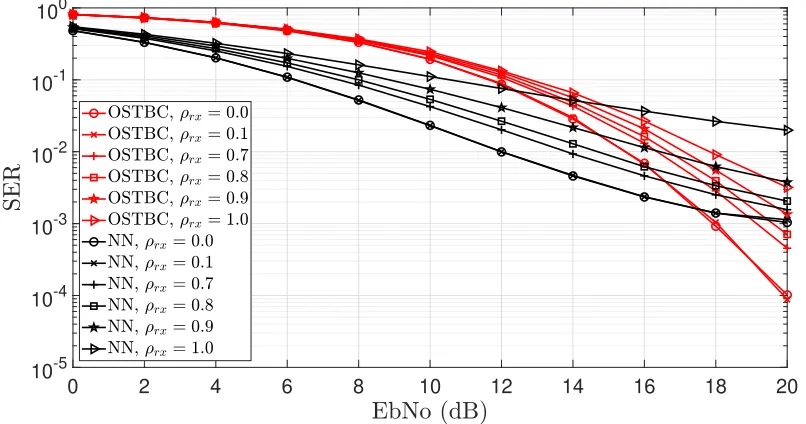
3.28 SER of3×3Scenario with Information rate of 4 bits/s with varying degrees of correlation induced among the receive antennas. The OSTBC serves as a baseline and employs perfect channel estimation at the receiver. . . 70
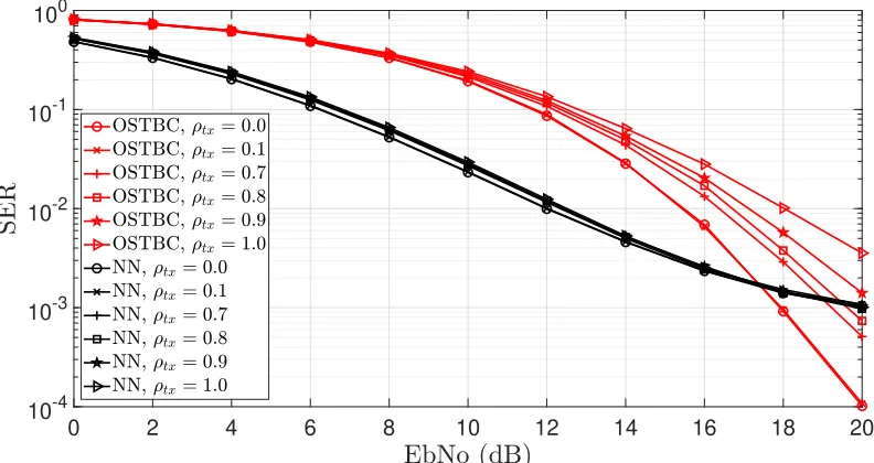
3.29 SER of3×3Scenario with Information rate of 4 bits/s with varying degrees of correlation induced among the transmit antennas. The OSTBC serves as a baseline and employs perfect channel estimation at the receiver. . . 71
3.30 SER of 3×3 MIMO Scenario with information rate of 4 bits/s trained on independent Rayleigh channels and tested across three different channels -Nakagami channel with an m factor of 0.5, Nakagami channel with an m
factor of 1, and Ricean channel with a Ricean factor of 4.5 . . . 72
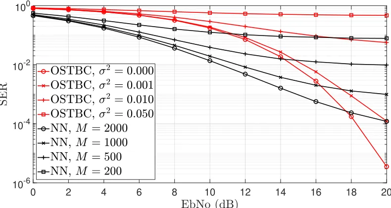
3.31 SER of 3×3 MIMO Scenario with information rate of 4 bits/s trained on independent Rayleigh channels and tested on a Nakagami channel with an m
factor of0.5. The impact of varying the decoding bach sizes of learned system is compared with the impact of channel estimation errors in the conventional OSTBCs . . . 73
3.32 SER of 3×3 MIMO Scenario with information rate of 4 bits/s trained on independent Rayleigh channels and tested on a Nakagami channel with an m
factor of 1. The impact of varying the decoding bach sizes of learned system is compared with the impact of channel estimation errors in the conventional
OSTBCs . . . 74
3.33 SER of 3×3 MIMO Scenario with information rate of 4 bits/s trained on independent Rayleigh channels and tested on a Ricean channel with a Ricean factor of4.5. The impact of varying the decoding bach sizes of learned system is compared with the impact of channel estimation errors in the conventional OSTBCs . . . 75
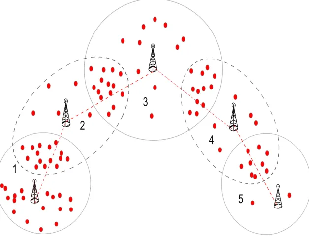
4.1 Cellular deployments with overlapping regions of coverage. The 5−th cell is uncongested, but the first cell has a lot of MTDs attached to it. The MTD-BS algorithm learns to distribute the MTDs in a manner that minimzes the overall network congestion. The dotted line depicts micro and pico cells. . . 78
4.2 Heterogeneous cellular network with seven Macrocells complemented with 3 picocells placed at the congestion hot spots. . . 84
4.3 Channel Utilization Ratio. . . 87
4.4 Channel Utilization Ratio for the 8−th Cell. . . 88
4.5 Channel Utilization Ratio for the 9−th Cell. . . 89
4.6 Channel Utilization Ratio for the 10−th Cell. . . 89
4.7 Channel Utilization Ratio for the 3−th Cell. . . 90
4.10 Learned redistribution of MTDs attached to Cell 8 to other δ−suitable cells 91
4.11 Probability of Collisions across all Cells. . . 92
4.12 Probability of Collisions for the8−th Cell. . . 93
4.13 Probability of Collisions for the9−th Cell. . . 94
4.14 Probability of Collisions for the10−th Cell. . . 94
4.15 Access Success Probability.. . . 95
4.16 Cumulative of the State Action Value that is Selected every Second by All MTDs while Following the MTD-BS off-policy Association Algorithm. . . 96
A.1 Channel Utilization Ratio for the 1−th Cell. . . 108
A.2 Channel Utilization Ratio for the 2−th Cell. . . 109
A.3 Channel Utilization Ratio for the 5−th Cell. . . 109
A.4 Channel Utilization Ratio for the 6−th Cell. . . 110
A.5 Channel Utilization Ratio for the 7−th Cell. . . 110
A.6 Probability of Collisions for the1−th Cell. . . 111
A.7 Probability of Collisions for the2−th Cell. . . 111
A.8 Probability of Collisions for the3−th Cell. . . 112
A.9 Probability of Collisions for the4−th Cell. . . 112
A.10 Probability of Collisions for the5−th Cell. . . 113
A.12 Probability of Collisions for the7−th Cell. . . 114
2.1 Alamouti Scheme . . . 14
2.2 OSTBC for 3 transmit antennas . . . 14
2.3 OSTBC for 4 transmit antennas . . . 14
2.4 Activation functions . . . 23
2.5 Loss functions . . . 24
3.1 Learned Transmitter - Neural Network Model . . . 48
3.2 Pre-processing - Neural Network Model . . . 52
3.3 Second Decoder Branch - Neural Network Model . . . 56
3.4 List Of Hyperparameters . . . 63
4.1 Simulation Parameters . . . 85
Chapter 1
Introduction
1.1
The Case for Learning-Based Systems
Although wireless networks have been extensively researched during the past decades, the promise of improved guaranteed quality of service, - reliability, and latency and new applications in future generation networks necessitates further investigation [1]. One area of possible research involves the modularized physical layer. Examples of the modular blocks include forward error correction, modulation, channel equalization, and orthogonal frequency division multiplexing. Over time, the optimization of these blocks has spawned into distinct and well-defined areas of research, and expert domain knowledge of these research areas has been established. Hence, recent research has yielded only marginal improvements in the performance gains, and most times these gains require complex analytical models that are intractable in real-world systems. Also, the modular structure of the physical layer may not be optimal, as is the case with the separation of modulation and coding [2].
However, in the machine learning world, model-free algorithms are being used to solve complex problems. Authors in [3], proposes a novel paradigm shift from the conventional design of the physical layer to an end-to-end machine-based design. This work led to a surge in the research of end-to-end machine learning-based systems. Leveraging this existing body of research, we aim to design space-time block codes that are more resilient to channel
impairments. Following previous works, we construct the transmit and receive aspects of the physical layer as a neural network. The symbols produced from the encoders are multiplexed in both space and time such that the final output is an integer multiple of the number of symbols in one time step. These symbol mappings are optimized by minimizing the mostly convex loss functions deployed in machine learning systems [4, 5]. We present our case by comparing our results with conventional space-time block codes which are submodular in design.
1.2. Current Trends 3
it can be very inefficient to explicitly schedule machine type devices.
We propose a multi-agent reinforcement-based solution. This solution exploits a het-erogeneous cellular network in order to alleviate the congestion caused by the simultaneous transmission of packets by a large number of machine the devices. Results from this scheme show that the MTDs are able to self-organize in a distributed manner across multiple cells in order to eliminate the long term congestion.
1.2
Current Trends
1.2.1
End-to-End Learning Based Diversity Systems
Multi-antenna systems have been in existence for more than half a century. Single Input Multiple Output systems based on receive combining has excited since the 1950s [6]. Multi transmit antenna systems (MISO) in [7], takes advantage of its time division duplex TDD implementation to support transmit based selection diversity. Although SIMO and MISO techniques had been popularized, the effect of simultaneously using multiple transmit and receive antennas was not known. Authors in [8], showed that with independent channel gains and antennas spaced sufficiently at both the transmitter and the receiver, the capacity increases linearly as the number of transmitters and receivers increased
area, and any machine-learning-based algorithm must have significant performance benefits, for it to be considered for implementation.
Noting this subtle, but important point, wireless researchers have tried to reinvent the communication wheel with machine learning-based techniques. Researchers in [12], designed a support vector machine (SVM) based link adaptation scheme. Using a frame by frame error computation, devices perform link adaptation to find the optimal rate/reliability trade-off. In [13], a deep neural network model is trained offline based on channel statistics and used online for symbol detection in orthogonal frequency division systems. A machine learning-based localization scheme is developed in [14]. Although promising, most of the previously stated research has focused on optimizing modular blocks of the physical layer. Recently, researchers postulated that representing the entire physical layer as a single block and performing a single optimization process could provide some performance benefits while simultaneously reducing the complexity of the communication systems.
1.2. Current Trends 5
1.2.2
Grant Free Resource Allocation for Machine Type
Commu-nications
Cellular networks have been proposed as a source of connectivity for machine-type devices. However, exploiting a network that was designed for human type communications for machine type communications has provided some interesting research challenges. An increasingly researched challenge is the random access procedure. Two challenges related to the application of the random access process to machine type communications are congestion and inefficiency. I) Congestion: Sensors measuring the same physical process could have similar transmit times. This will lead to an increase in congestion and subsequently a high rate of collisions in random access. II) Efficiency: MTDs generate packets that are small relative to the number of resource blocks used in the RA process. Therefore, it is inefficient to use the random access process to transmit packets of such sizes. Previous resource allocation solutions for MTDs can be grouped into coordinated access and grant free schemes.
Coordinated access schemes
1.2. Current Trends 7
Grant-free schemes
1.3
Thesis Organisation and Contributions
This thesis consists of two parts. The first part involves modeling the physical layer as an autoencoder in order to generate new space-time block codes. The second part of this thesis involves applying reinforcement learning in order to reduce the congestion caused by a massive number of machine-type devices. More specifically:
• In the first part of this thesis, we expand on previous autoencoder models for the physical layer [3]. We show through simulations that we can eliminate the need for explicit pilots and channel estimation in space-time coding if we design the receiver as two distinct blocks. The first block called the pre-processing block extracts the complex values needed for combining from a batch of received symbols. This block also performs some sort of pseudo-combining at the receiver, after which the second block estimates the symbols sent at a specific time.
• We compare the symbol error rate performance obtained from the neural network based space-time coding scheme with the symbol error rate performance derived from classic orthogonal space-time block codes.
• In the second part of this thesis, we formulate the congestion problem caused by the concurrent transmissions from a massive number of machine type devices as a constrained combinatorial problem. We claim that the problem is intractable due to a lack of information at the base station.
• The optimization is reformulated as a finite MDP. We approximate the solution of the MDP using a distributed model-free algorithm.
1.3. Thesis Organisation and Contributions 9
the optimal solution when the number of MTDs is less than the number of time slots.
1.3.1
Organization
Background
In order to to fully appreciate the work presented in this thesis, we provide background material in this chapter for several key concepts. First, we provide an introductory overview of multi-antenna systems and the muliplexing/diversity beneifts they provide. Second, we present a discussion about the type of communication devices that are regarded as ”ma-chine type” devices and we briefly present a discussion on the suitability of using cellular networks in order to provide connectivity for machine type communications. We highlight that the random access protocol is a bottleneck in the deployment of cellular networks for machine type connections. Third, because, most contributions made in this thesis are in the area of machine learning and/or reinforcement learning, we provide a definition and a simple introduction to the fundamental principles behind machine learning. More specifi-cally, we define the various terms and discuss the different classifications of machine learning algorithms. A simple discussion is presented about the limitations and failings of machine learning algorithms. However, we also show that deep learning models are powerful function approximators used to learn relationships that are too complex for conventional machine learning methods. Along with an overview of how the neural models are stacked in order to generate a deep learning system, a discussion of the expressive elements needed for each neural element is presented. In addition, we present a brief reinforcement learning overview. A discussion is presented regarding model and model-free reinforcement learning approaches. This section concludes with a description of the popular Q-learning algorithm deployed in
2.1. Multi-antenna Systems 11
chapter 4.
2.1
Multi-antenna Systems
Signal processing techniques that deploy multiple antennas at the transmitters and/or receivers are described as Multi Input Multi Output systems (MIMO). The additional degree of freedom present in communication systems due to multiple antennas is used to either im-prove system throughput or system reliability. MIMO techniques that exploit the additional degrees of freedom to increase throughput are referred to as spatial multiplexing. Spatial multiplexing takes advantage/exploits the rich multipath scattering in communication chan-nels to increase the rate at which information is transmitted from one point to another. The other class of MIMO techniques combats the multipath effect of the communication channel in order to increase system reliability. These systems are termed diversity achieving systems. Although, MIMO is commonly used to refer to any system with multiple antennas at both the transmitter and the receive, some authors abuse this terminology and refer to systems with more than one antenna at only one side of the communication link as MIMO systems. In the strict sense, a communication model deployed with single transmit and mul-tiple receive antennas is called SIMO - single input multi output. Similarly, a model with a single-receive multi-transmit configuration is called MISO - multiple input single output. Finally, in the literature a system model withNttransmit antennas andNr receive antennas
is denoted as a Nr×Nt MIMO system.
The medium between the Nt transmit antennas and Nr receive antennas is referred to
characterizes the rapid fluctuation of signal strength over short distances and/or over a short period of time. Small scale fading occurs when the transmitted signal arrives along different paths, each path having its own inherent phase, Doppler shift, delay, and path attenuation. This category of fading can be further categorized dependent on the bandwidth of signal transmitted. A signal with bandwidth greater than or on the same order as the channel co-herence bandwidth will experience frequency-selective fading, which leads to complications during demodulation. A simple solution is to use orthogonal frequency division multiplexing (OFDM) to divide the signal into many narrowband signals. A channel with a short coher-ence time (or a large Doppler) is termed a fast fading channel. Hcoher-ence, fades will last for only a short period of time. II) Large scale fading occurs on a much longer time scale and over longer distances. Large scale fading is used to characterize the loss in signal amplitude due to the terrain of the environment.
2.1. Multi-antenna Systems 13
techniques include: I) Selective combining: this technique involves selecting one of he received signals based on some metric. Most authors use the signal to noise ratio (SNR) as the metric of choice. II) Maximum ratio combining: this involves weighing the various received signals based on their SNR’s and combining them. The weights are designed such that signals with better SNR are given a higher weight. III) Equal gain combining - This is a special version of maximum ratio combining with the caveats that all the weights are set to the same value. The discussed diversity techniques are referred to as receive diversity. It gets this terminology because processing and combining are done by the receiver. The performance of a receive diversity system is heavily dependent on how far apart the receive antennas are spaced. The farther apart the antennas are the more independent the fades. However, in cellular communications, engineers are limited by the available space. This is because mobile phones have a size beyond which they are impractical. This motivates the need for transmit diversity in the forward link or cellular downlink. However, achieving transmit diversity is a nontrivial task. Consider a multi transmit single antenna system, simply sending the same signal across all antennas doesn’t provide diversity. To see this, consider the output of a matched filter with a single receive antenna:
r= √s
s
Nt X
i=1
hi+n (2.1)
In this equation, r, represents the received signal sample at the output of our matched filter, hi denotes the channel between the receiver and thei−th transmitter, s is the
space-time coding. The most popular type of space-time coding for two transmit antennas is known as the Alamouti scheme. This scheme has attracted much popularity because it is the only rate one space-time block coding scheme for complex modulation. This means that on average one symbol is transmitted every time a step. At the receiver, maximum
Table 2.1: Alamouti Scheme
Time Index Antenna 1 Antenna 2
t s1 s2
t+Ts −s∗2 s∗1
ratio combining is used to realize the diversity benefits. A common space time block code for higher number of transmit antennas is the orthogonal space time block coding (OSTBC) scheme [10] which is a generalization of the Alamouti scheme and is shown in Tables2.2 and 2.3 for 3 and 4 antennas respectively. These codes gained popularity because the authors provided a decoding scheme which is linear in processing time.
Table 2.2: OSTBC for 3transmit antennas
Time Index Antenna 1 Antenna 2 Antenna 3
t s1 s2 0
t+Ts −s∗2 s∗1 0
t+ 2Ts 0 0 s1
t+ 3Ts 0 0 −s2
Table 2.3: OSTBC for 4transmit antennas
Time Index Antenna 1 Antenna 2 Antenna 3 Antenna 4
t s1 s2 0 0
t+Ts −s∗2 s∗1 0 0
t+ 2Ts 0 0 s1 s2
t+ 3Ts 0 0 −s∗2 s∗1
2.1. Multi-antenna Systems 15
that can be effectively sent over such a channel ismin{Nt, Nr}. Notice that in spatial
multi-plexing, multiple streams are sent over the same frequency resource at the same time, hence, this technique increases throughput without increasing the required bandwidth. In an SM-MIMO system, a precoder is used to map the stream of input data to the multiple transmit antennas. The precoder can be a simple serial to parallel converter. In eigenbeamforming, the precoder is a function of the communication channel and thus requires feedback from the receiver.
have a channel with a rank of 2, regardless of the number of transmit and receive antennas, we can only send two effective data streams.
2.2
Machine Type Devices
2.2. Machine Type Devices 17
2.2.1
Random Access
When a UE migrates into a region with cellular coverage, its first job is to synchronize with the base station (gNodeB). In order to achieve this task, it needs to decode the primary synchronization signals (PSS) and secondary synchronization signals (SSS). The former is responsible for slot synchronization while the later is responsible for frame synchronization. The PSS and SSS are both present in the 1st and 11th slots in every frame. The PSS occupies the last OFDM symbol in both slots, while the SSS is present in the symbol before the PSS.
Due to the two UEs selecting the same preamble and transmitting at the same time, they have the same random access-radio network temporary identifier-1 (RA-RNTI-1). For simplicity, we assume that UE-2 loses out on this contention, i.e, the gNB correctly detects the preamble for UE-1, and fails to detect the preamble of UE-2. The gNB estimates the uplink transmission timing of UE-1 and derives RA-RNTI-1. Subsequently, an identifier (cell-RNTI) is assigned to UE-1, and this identifier serves as a placeholder used in addressing UE-1. The two UEs both tune to the physical downlink control channel (PDCCH) and receive the downlink control information (DCI). This information is addressed to RA-RNTI-1. The gNB provides the RA response on the DL-SCH. This RA-response carries the following: temporary C-RNTI-1, Timing Advance, Uplink Resource Grant. It should be emphasized that both UEs receive this message because it is addressed to RA-RNTI-1. Both UEs save the temporary C-RNTI-1 and they both apply the timing advance.
UE-1 and UE-2 don’t have a permanent identity, hence, they independently generate two separate random numbers to represent their identities. They include this random identity in their respective radio resource control (RRC) connection request.
2.2. Machine Type Devices 19
transmission from UE-1 and sends an ACK in (Acknowledgment). A resource assignment is made using the C-RNTI-1. An RRC Connection Setup message addressed with C-RNTI-1 is also sent by the gNB. Both UEs receives these messages.
The RRC Connection Setup addressed by C-RNTI-1 also contains the random number generated by UE-1. UE-1 notices the equivalence between the random number it gener-ated and the random number it received and it sends a Hybrid ARQ. The RA process has succeeded for 1 and it stops its T300 timer. Uplink resource requests are made by
The random number generated by UE-2 and that in the connection setup received by UE-2 don’t match. Since, UE-2 can’t confirm its identity, UE-2 realizes it has lost the contention. UE-2’s T300 timer ends and it retries the random access process. It should be noted that each random access slot has a size of 1.08MHz (six resource blocks).
2.3
Introduction to Machine Learning
Any algorithm that accepts and learns from data, such that it gets better at performing some task, T can be classified as a machine learning algorithm. The performance is measured and evaluated by a quantitatively defined-metric. Tasks that are difficult to model and solve but for which there is ample data are perfect candidates for a machine learning (ML) algorithm. A common misuse of terminology among researchers is to assume ”learning”, ”task” and ”training examples” all mean the same thing. To buttress the differences among these terms, consider an autonomous vehicle that has been trained to perform maneuvers on the highway. Performing maneuvers is the task, the data captured by the vehicular sensors which are usually in the form of pixels are the examples. More specifically, the distinct examples are defined by a feature vector, such that x ∈Rp, wherein this case, p represents the number of RGB values characterizing each image. A collection of examples is easily specified by a matrix X ∈ Rn×p. After specifying the task and collecting examples, we can
write a learning algorithm or we can write a deterministic program to provide the vehicular nodes with maneuvering capabilities.
A common trend among machine learning researchers is to classify machine learning problems according to its intended task. A common classification of ML problems is: I) Classification problems: Classification problems involves learning a function mapping f :
2.3. Introduction to Machine Learning 21
places the sample in one of k distinct groups. A popular example of such a problem is the identification of animals in pictures. In this problem, a sample example has a feature vector of RGB values and the output is a numerical value defining various classes. II) Regression problems: In this problem, given a training sample, an algorithm is tasked with predicting a continuous numerical value. Mathematically, the algorithm learns the function mapping
f : Rp −→ R. A common and non-trivial example is predicting the price of future stock options, given a set of past examples {X,y}, such that X represents examples and their feature vectors and y represents the corresponding past stock prices.
Another common discriminator of ML problems pertains to the mode of learning. Broadly speaking, the two types of learning algorithms are unsupervised learning and su-pervised learning algorithms. I) Susu-pervised algorithm: Consider a function y = f(x), a supervised learning algorithm finds an association from the training inputs denoted by x to corresponding labels y. This association is used to predict label values for previously unseen test data. Examples of supervised learning algorithms include linear regression, lo-gistic regression, and support vector machines. II) Unsupervised learning: The fundamental difference between unsupervised and supervised learning is the absence of a target/label in the former. Unsupervised algorithms attempt to extract information about the underlying data distribution of the training samples. The algorithms learn to cluster training samples with related features into distinct groups. When a new test sample is provided, the al-gorithm must determine which group placement is most suitable for this previously unseen data. Examples of unsupervised learning include principal component analysis andk−means clustering. The authors in [45] present an extensive discussion on machine learning concepts.
as the curse of dimensionality. The increase in dimension size (length of feature vector) leads to an exponential increase in the number of possible different feature configurations and the probability that some configurations will not have an associated training example increases. Hence, the output of such examples needs to be approximated. This fundamental problem motivates the need for deep learning.
2.3.1 Deep Learning
Deep learning models are universal function approximators. Consider a function, f∗ which denotes the relationship between a datasetX, and its targety. A deep learning model attempts to use the dataset {X,y} to learn a set of parameters, θ which approximates the functionf∗. A deep learning model produces the mappings,≈y=f∗(x). Although there are other types of deep learning models, in its most basic form, the output of the deep learning model has no feedback loop and it is called a feedforward network. In practice, feedforward models have many layers and can be viewed as functions of functions.
f(x) =f(l)(· · ·f(2)(f(1)(x))) (2.2)
The functions f1 ,f2 , and fl denotes the first, second, and output layers respectively.
A single layer of the feedforward models also known as a perceptron and can be described with the following function:
yl = Φl(Wlxl−1+bl) (2.3)
The weights, Wl ∈RNl×Nl−1, and the biases, bl ∈RNl, terms are the trainable param-eters of the l−th layer - θl = {wl,bl}. The input into the l−th layer, xl ∈ RNl−1, is the
2.3. Introduction to Machine Learning 23
followed by a nonlinear activation function. The non-linearity of the activation functions is the expressive power of the neural networks.
Table 2.4: Activation functions
Name Function Φ(q) Range
Linear qi (−∞,∞)
TanH tanh(qi) (−1,1)
RELU [46] max(0, qi) [0,∞]
Leaky RELU [47]
(
αq, for q <0
q, for q ≥0 [−∞,∞)
Sigmoid 1
1+e−q (0,1)
ArcTan tanh−1(qi) (−∞,∞)
ELU [48]
(
q, for q >0
αeq−α for q ≤0 (0,∞)
SoftPlus [49] In(1 +exp(q)) (0,∞)
SoftMax [50] eqi
∑j=N j=0 e
qj (0,1)
Swish [51] 1+qe−q (0,∞)
In the absence of this expressive power, there would be no real gain in using a multiple layered neural network. The activation function operates on its input vector, by operating independently on each of its elements. Hence, [Φ(q)]i = Φ(qi). Table 2.4 presents a
neural network operation.
Table 2.5: Loss functions
Name l(ˆy,y)
Binary Entropy Loss −ylog(ˆy)−(1−y)log(1−yˆ)
Minimum Squared Error ∥(ˆy−y)∥2
Minimum Absolute Error |(ˆy−y)|
Cross Entropy Loss −PM
j yjlog(ˆy)
The loss function produces a comparison between the neural network approximations,
ˆ
y, and the target variables, y. Table 2.5 provides examples of common loss functions. It should be noted that the loss functions are application/problem specific. In Regression-based deep learning applications, both the target variable, y, and the estimates produced by the neural networkyˆ are continuous and real-valued, hence the minimum squared and minimum absolute error are suitable loss functions. For classification problems, the neural network produces a continuous real number between the range (0,1). This restriction in the range is usually enforced by applying the sigmoid (binary classification) or softmax (multinomial classifications) activation functions. The target variables in classification problems are either 1,0, i.eyi ∈ {0,1}. In practice, this value is one-hot encoded such that the target vector for
2.3. Introduction to Machine Learning 25
Figure 2.1: A RELU Activation Function.
Figure 2.3: The Sigmoid Activation Function.
2.3. Introduction to Machine Learning 27
The backward pass entails propagating the loss from the outermost layer throughout the entire network in order to update the parameters of the neural network. The popular back-propagation algorithm provides an intuitive way of achieving this [52]. At a time t+ 1, with a learning rate, γ, the back-propagation algorithm can be described with the following equation:
θt+1 =θt−γ
∂l(ˆy,y)
∂θt
(2.4)
Although gradient descent has shown good performance [53, 54], researchers have re-cently proposed other propagation algorithms. Authors in [55], improve upon the gradient descent algorithm by dynamically updating the learning rate. This method is referred to as momentum, and provides gradient stability and accelerates descent across regions of low steepness. A simple parameter update with gradient descent and momentum is shown in Equation 2.5:
Qt+1 =βQt+ (1−β)
∂l(ˆy,y)
∂θt
θt+1 =θt−γQt+1
(2.5)
β ∈[0,1]is a hyperparameter that can be used to tune the performance of the learning system. Recently, the Adam algorithm [56] has seen its popularity increase among researchers over the past couple of years. This popularity is due to its ability to deal with stochastic objective functions while maintaining a simplistic implementation. The algorithm can be written using the following weight update:
2.3. Introduction to Machine Learning 29
t←t+ 1
mt ←β1mt−1+ (1−β1)∂l(ˆ
y,y)
∂θt−1
qt←β2qt−1+ (1−β2)(∂l(ˆ
y,y)
∂θt−1 ) 2
˜
mt ←mt/(1−β1t) ˜
qt←qt/(1−β2t)
θt←θt−1−γm˜t/(
√ ˜
qt+ϵ)
end while
The (∂l∂θ(ˆy,y)
t−1 )
2 term represents elementwise squaring of the gradient vector. In addition,
to the learning rate, γ; β1, β2 ∈[0,1] and ϵ are also hyperparameters. For much of chapter
3, a deep neural model is employed and optimized through the Adam algorithm.
2.3.2
Reinforcement Learning
A novice would be forgiven for expecting previously discussed learning techniques to be all-encompassing of all the available learning techniques, but this is not the case. A special class of learning involves mapping circumstances to actions, in order to ensure that a nu-merical reward is being maximized. This category of learning is referred to as reinforcement learning. This model depicts a learner that can start off as myopic and sequentially becomes intelligent by leveraging its past experiences. A reinforcement learning system has no in-struction manual, the learner is never told what to do, however, the system is designed as a closed-loop system such that the learner can receive numerical feedback on the consequences of its actions.
predict the label of previously unseen data. Clearly, these parameters are trained to gener-alize, however, in interactive systems where the actions predicted by the algorithm generates new training samples and a new action sample space, it becomes important that learning sys-tems have the ability to sequentially improve their parameters through experiences. To solve this problem, reinforcement learning models are used to learn from their past experiences. Obviously, learning from experience implies that the learning system must have a target goal and behavior. The target goal of any reinforcement learning problem is completely described by a reward signal. Reinforcement learning is supposed to provide an intuitive solution to the conundrum of goal-based learning from interaction.
In practice, reinforcement learning solutions are usually framed as Markov decision processes (MDPs). The formulation of a Markov decision process can be divided into an agent and its environment. The agent makes decisions based on a full or partial observation of the environment. The environment responds to the decisions by providing both a reward signal and new environmental situations to the agent. More concisely, at a discrete-time step, t, an agent observes either a full or partial representation of the environment, St ∈S.
Through a stochastic or deterministic policy conditioned on this observation π(at|st), an
action is selected, At ∈A(St). Note that, S, is the set of all possible states and A(St)is the
set of all possible actions provided that we are in state, St. Subsequently at the next time
step, the agent receives a numerical reward,Rt+1 ∈R and transitions into a new state St+1.
distribu-2.3. Introduction to Machine Learning 31
tions. These random variables exhibit the Markov property:
p(s′, r|s, a) =P r{St=s
′
, Rt =r|St−1 =st−1, At−1 =at−1} (2.6)
where, s′ denotes the future state. The Markovian property implies that current states include all the past information which would influence future states.
X
s′∈S
X
r∈R
p(s′, r|s, a) = 1,∀s∈S, a∈A(s) (2.7)
In Equation 2.6, p is a probability variable denoting the dynamics of the Markov decision process. With the Markovian property and the dynamics variable, we have all the information pertaining to the environment, and any relevant information can be generated. For example, the state transition probabilities can be computed with
p(s′|s, a) =X
r∈R
p(s′, r|s, a) (2.8)
while, the reward for a specific state action pair can be computed as
r(s, a) =X
r∈R
rX
s′∈R
p(s′, r|s, a) (2.9)
In order, to formally and mathematically define the reward structure, consider the reward received from the environment after time step t: Rt+1, Rt+2,· · · , RT, where T indicates
the final time step. The question arises: how do we want to maximize this sequence? An intuitive answer would be, to maximize the sum of the total sequence. This sum of sequential rewards is a simple form of the return.
This naive approach could work well for a sequence with a finite length, T < ∞. For such sequences, the task ends when the agent moves into a terminal state, S∗. Reinforcement learning problems that cause agents to interacts with environments such that the generated sequence of states ends in a terminal state are termed episodic tasks and the resulting sequences are referred to as episodes. In contrast, tasks that are designed in such a way that there are no terminal states are referred to as a continuing task. For continuing tasks, the sum of the total reward would be infinite, hence researchers introduced a discounting factor, γ. In a continuing task, the agents select actions that maximize the cumulative sum of its immediate reward and a discounted sum of all future rewards.
Gt =Rt+1+γRt+2+· · ·= ∞ X
k=0
γkRt+k+1 (2.11)
Equation 2.12 presents a generalised definition of the return. The discount factor can only take values between zero and 1, 0 ≤ γ ≤ 1. With a discount factor of zero, the agent only considers immediate reward, and as this factor is increased from zero to one, the agent becomes less myopic. However, a necessary condition for boundedness isγ <1. The return can be recursively written as:
Gt =Rt+1+γGt+1 (2.12)
2.3. Introduction to Machine Learning 33
an agent can accrue if it starts out at that state and follows a certain policy, π.
vπ(s) =Eπ[Gt|St=s] =Eπ
" ∞ X
k=0
γkRt+k+1|St=s
#
,∀s∈S (2.13)
Likewise, an action value function can defined as the expected future return if an agent starts at a state, St∈S takes action,At ∈A and subsequently follows a policy,π.
qπ(s, a) = Eπ[Gt|St=s, At =a] =Eπ
" ∞ X
k=0
γkRt+k+1|St=s, At =a
#
(2.14)
From equations 2.13 and 2.14, the state value function is derived by averaging all its action values.
vπ(s) =
X
a′∈A(s)
π(a′|s)qπ(s, a
′
) (2.15)
Similar to the return function 2.12, the value and action functions of a specific state has a recursive relationship with its successive states.
vπ(s) =Eπ[Gt|St =s]
vπ(s) =Eπ[Rt+1+γRt+2+· · · |St =s]
vπ(s) =Eπ[Rt+1+γGt+1|St=s]
vπ(s) =Eπ[Rt+1|St=s] +Eπ[γGt+1|St =s]
(2.16)
vπ(s) =Eπ[Rt+1|St =s] +γEπ[Eπ[Gt+1|St+1]|St=s]
vπ(s) =Eπ[Rt+1|St =s] +γEπ[vπ(st+1)|St=s]
vπ(s) =Eπ[Rt+1+γvπ(st+1)|St =s]
(2.17)
Similarly, the action value function can be expressed as
qπ(s, a) = Eπ[Gt|St=s, At=a]
qπ(s, a) = Eπ[Rt+1+γRt+2+· · · |St=s, At=a]
qπ(s, a) = Eπ[Rt+1+γGt+1|St=s, At=a]
qπ(s, a) = Eπ[Rt+1|St=s] +Eπ[γGt+1|St=s, At =a]
(2.18)
Again with the law of total expectation
qπ(s, a) = Eπ[Rt+1|St=s] +γEπ[Eπ[Gt+1|St+1]|St=s, At=a]
qπ(s, a) = Eπ[Rt+1|St=s] +γEπ[vπ(st+1)|St =s, At =a]
qπ(s, a) = Eπ[Rt+1+γvπ(st+1)|St=s, At =a]
(2.19)
The last equation in 2.17 and 2.19 denotes the Bellman equation forvπ and qπ
respec-tively. Notice that the bellman equations are dependent on the policy,π. Hence, for a finite MDP we can take advantage of the bellman equations in order to define an optimal policy,
π∗. More specifically, a policy π∗ is better than every other policy, π, if the value function vπ∗(s)∀s derived by the following policy, π∗, is equal or greater than the value functions
derived from following any other policy, vπ(s) ∀s. Although every finite MDP has an
2.3. Introduction to Machine Learning 35
functions termed the optimal state-value function, v∗.
v∗(s) =max
π vπ(s) (2.20)
Obviously, the optimal state value function is equivalent to the expected return derived by selecting the action with highest action value.
v∗(s) = max
a∈A(s)qπ∗(s, a)
v∗(s) = max
a Eπ∗[Rt+1+γGt+1|St=s, At=a]
v∗(s) = max
a Eπ∗[Rt+1+γv∗(St+1)|St=s, At =a]
v∗(s) = max
a
X
s′,r
p(s′, r|s, a) [r+γv∗(St+1)]
(2.21)
The Bellman optimality equation forv∗(s)is represented by the last two equations . Similarly, the the optimality eqaution for q∗(s) is
q∗(s, a) = E
Rt+1+γmax
a′
q∗(St+1, a
′
)|St=s, At =a
(2.22)
ex-pected return of each state-action value pair. Considering this, we still have the problem of obtaining the optimal action/state value functions. Since the Bellman equations represent a nonlinear system of equations, this problem can be solved through various readily available techniques. However, explicitly solving the Bellman optimality equations is analogous to performing an exhaustive search and this search depends on the following:
• We have full knowledge of the system dynamics, p.
• We have enough computation resources to evaluate all states.
Clearly, for most real-world problems with a high number of possible states, these assump-tions are not applicable. Consequently, researchers usually settle for approximate soluassump-tions. Two examples of popular reinforcement learning approximations will be discussed in the following sections.
Dynamic Programming
2.3. Introduction to Machine Learning 37
vk+1(s) = Eπ[Rt+1+γvk+1(st+1)|St =s]
vk+1(s) =
X
a
π(a|s)X
s′,r
p(s′, r|s, a) [r+γvk+1(st+1)]
(2.23)
It is important to state that regardless of the initial state-value, v0, the sequence,v0, v1,· · ·
converges to vπ in the limit. Equation 2.23 operates by successively approximating the new
state-value function from both the immediate reward and all possible previous successor states value function. The iterative policy evaluation algorithm is discussed below. Notice that, since this method only converges in the limit, a stopping criterion is usually imposed in practice.
Algorithm 1: Iterative Policy Evaluation
Result: The approximated state-value function V a(s)
Initialize the policy, π, the stopping criterion,δ and the state-value function,
V a(s)∀s ; while δ >Ω do
Ω←0;
foreach s∈S do
v ←V a(s) ;
V a(s)←Paπ(a|s)Ps′,rp(s′, r|s, a)r+γV a(s′);
Ω←max(Ω,|v−V a(s)|) ; end
end
policy, a = π′(s) ̸= π(s), and subsequently follow the existing policy, π. This is defined mathematically as
qπ(s, π
′
(s)) =Eπ[Rt+1+γvπ(St+1)|St=s, At=a]
qπ(s, π
′
(s)) =X
s′,r
p(s′, r|s, a)
h
r+γvπ(S
′
)
i (2.24)
If the action value function calculated in this way is greater than the current state value function derived form following policy,π, when in-states, then it would be better to always selecta=π′(s)whenever this state is encountered. This idea is a simplification of the policy improvement theorem. The policy improvement theorem states, for all states, s∈S, if there are two nonstochastic polices, π and π′, which returns:
qπ(s, π
′
(s))≥vπ(s) (2.25)
then
vπ′(s)≥vπ(s) (2.26)
This theorem paves the way for iterative policy improvement. If we consider a new policy described as:
π′(s) =arg max
a qπ(s, a) (2.27)
2.3. Introduction to Machine Learning 39
function of the old policy,vπ′(s) = vπ(s)then from Equation 2.27, we have:
vπ′(s) =max
a Eπ[Rt+1+γvπ(St+1)|St=s, At=a]
vπ′(s) =max
a
X
s′,r
p(s′, r|s, a)
h
r+γvπ(S
′
)
i (2.28)
Clearly, this equation is equal to the Bellman optimality equation 2.21. Therefore, both the new and old policies are optimal, vπ′(s) = v∗(s). We can conclude that an iteration of policy evaluation will generate a strictly better policy except when the old policy is already optimal. This fact provides us with the policy iteration algorithm.
The policy iteration algorithm can be described as:
• Upon evaluating a policy, π, through its state value functions, vπ(s).
• We improve this policy by acting greedily with respect to the new value functions - we get a new policy π′.
• We evaluate this policy to get its state value functions, vπ′(s).
• This policy is improved again by taking greedy actions, this results in a new policy,π′′
• Once again this policy is evaluated to get, vπ′′(s).
• This process is continued until policy evaluation generates a policy, such that the new state value functions and the previous state value functions are equal and therefore optimal.
The pseudo-code for this algorithm can be found in [57]. It is clear that every sequence of policy iteration involves evaluating the current policy, vπ. However, since vπ is derived
formulation of another class of solutions referred to as value iteration. Value iteration is a special kind of policy iteration where the policy evaluation is truncated after a single sweep of all the states. Surprisingly, the value iteration equation is equivalent to transforming the Bellman optimality equation into an update rule:
vk+1(s) =max
a Eπ[Rt+1+γvk(St+1)|St=s, At=a]
vk+1(s) =max a
X
s′,r
p(s′, r|s, a)
h
r+γvk(s
′
)
i (2.29)
The value iteration algorithm aggregates a single policy evaluation iteration with a single pass of policy improvements. The complete pseudo-code for value iteration is found in [57]. Although policy and value iteration provides a method of both policy evaluation and policy improvement, they are both constrained due to their dependence on the availability of the system dynamics. In other words, dynamic programming methods are dependent on the complete knowledge of the system model. Since a derivation of the complete system dynamics are usually intractable for most interesting problems. Model-free solutions are used to circumvent this challenge by approximating the system dynamics from experienced data.
Model Free Algorithms
Model-free algorithms are usually classified as either: I) Monte Carlo based (MC) algo-rithms or II) Temporal Difference (TD) algoalgo-rithms. TD and Monte Carlo algoalgo-rithms update an estimate,V of the actual value functions, vπ, based on experiences gained by following a
2.3. Introduction to Machine Learning 41
approximate the actual state value function given by Equation 2.17 as
V(St) =V(St) +α[Gt−V(St)] (2.30)
MC methods can be slow since the learning episodes could take a long time to terminate. Temporal difference algorithms provide a simple alternative. TD algorithms provide an update by bootstrapping the current return, Rt, with an estimate of the next state action
value, V(St). In other words, temporal difference learning approximate Equation 2.17, as
V(St) = V(St) +α[Rt+1+γV(St+1)−V(St)] (2.31)
As with dynamic programming, after evaluating the state value function derived from a policy, π, the next step is to improve on that policy. However, unlike dynamic programming the state value functions are not sufficient for policy improvement. With a model (dynamic programming), during policy improvement, a simple look-ahead provides the best action to take in order to achieve the maximum reward. Without a model, this simple look ahead is not possible without computing the action-value functions. Hence, model-free methods are largely dependent on estimating the action-value functions, Q(St, At). Estimating the
state-value functions through TD learning can be described as
Q(St, At) =Q(St, At) +α[Rt+1+γQ(St+1, At+1)−Q(St, At)] (2.32)
Notice that if the policy which generates the next action, At+1 is deterministic,
this undermines the entire goal of learning. To solve this problem and ensure that all state-action pairs are visited, a probabilistic constraint is usually imposed on the learning process. This constraint demands that at every time step, the agent has a non-zero chance of picking every possible action. The manner in which this constraint is imposed defines two classes of learning: I) on-policy: here, the agent attempts to improve the policy used to generate the St, At, Rt, St+1 sequence, and II) off-policy: the agent improves a policy that
is different from the policy producing the sequence transitions. In its most simplified form, the on policy update scheme for TD learning is given by Equation 2.32, with the slight modification, that the next action, At+1, need for bootstrapping is derived according to,
At+1 ←
arg maxaQ(St+1, a), With probability 1−ϵ
any action a, With probability ϵ
This is referred to asϵ-greedy
selec-tion, with optimization hyperparameter, ϵ. The resulting algorithm is referred to as Sarsa [57]. The off-policy TD algorithm [58] has a slight modification.
Q(St, At) =Q(St, At) +α
h
Rt+1+γmax
a Q(St+1, a)−Q(St, At)
i
(2.33)
Chapter 3
Learning Based Multi-Antenna
Transmission Systems
The modularized nature of communication systems has proved an efficient and effective model. However, researchers have recently investigated the possibility of exploiting potential gains by combining the modularized functions into a single function [3]. A feedforward autoencoder system presents us with a method of achieving this goal. To this end, this chapter investigates the possibility of an end to end diversity achieving system for different transmit and receive configurations.
To present a learned diversity system for combating the effects of a previously unknown channel, we train the learned system offline by providing the encoder with a batch of symbol indices, the encoder produces symbol representations for each index. The number of repre-sentations generated depends on both the designated number of transmit antennas and the code rate. The symbols are passed through the multiplicative effects of a Rayleigh channel and additive effects of Gaussian noise. At the decoder, the original symbols are extracted. Subsequently, the loss is computed through a suitable convex loss function, and backpropa-gation is used to update the weights of both the encoder and decoder. For training purposes, we use offline training which makes this backpropagation possible. During testing, random and previously unseen instantiations of the channel are used to evaluate the symbol error rate at the varying signal to noise ratios. This allows us to determine if the system has
generalized the response to the wireless channel. The noise power is used to vary the signal to noise ratio.
The transmitter design mandates that a matrix of complex representations is generated for each symbol index. This unique structure employs us to investigate the possibility of combating the impact of channel correlation at both the transmit and receive antennas. To investigate the impact of correlation, we train the encoder and decoder with independent instantiations from a Rayleigh distribution. After training, the learned system is tested in the presence of correlation at either the transmit or receive antennas. Our results indicate that while the performance of the learned system is not hampered by correlation among the transmit antennas, it degrades substantially with correlated receive antennas.
3.1. System Model 45
3.1
System Model
A learned system - completely described by a neural network - tries to communicate one out of a possible of T = 2k symbols. The learned system can be visualized as a three-part system consisting of the encoder/transmitter, decoder/receiver, and the channel [see Figure 3.1].
Transmitter Receiver
Sink Source
Channel
NN-Decoder NN-Encoder
Channel
S x y
ŝ
Figure 3.1: Autoencoder-Based System Layout.
circumvent this by by-passing the channel during backpropagation. The gradient from the input neural layer of the decoder is passed to the output layer of the encoder. This operation is plausible because backpropagation is carried out by the product rule. During learning, a symbol, s is fed into the encoder and reconstructed at the decoder, s. The autoencoder isˆ
modeled with a deep feedforward neural network, the weights and bias are modeled with a parameter θ. The encoder operation is described by the following function.
S =fT(s;θT) (3.1)
Each symbol,s, is encoded by the transmitter parameters,θT, across space and time to form
a matrix of symbols
Si =
˜
s11 s˜12 . . . s˜1K
˜
s21 s˜22 . . . s˜2K
... ... . .. ...
˜
sNt1 s˜Nt2 . . . s˜NtK (3.2)
where the matrix S ∈ CN t×K, and its individual entries s˜
jl represent the learned
representation on the j−th antenna at the l−th time instants. Clearly, every input symbol to the transmitter occupies K different channel uses. Hence, the symbol code rate is easily specified by 1
K. At a single time instant, a single column of the matrix in Equation 3.2
is transmitted. We define such a column as x. The received signal at each time instant, modeled asyi =Hix+ni, wherex∈CN t,Hi ∈CN r×N trepresents the channel impairments
modeled by Rayleigh fading, and ni ∈CN r represents Gaussian noise. The decoder has two
3.1. System Model 47
vector, where the components of v represent the estimated posterior probabilities for each possible message. The decoder operation can be represented using the following function:
v=fR(Y;θ) (3.3)
Finally, the symbol is estimated as sˆ=arg maxi[v]i. [v]i, denotes the i−th element of
3.1.1
Deep Learning Based Transmitter Design
The transmitter is designed using a feedforward neural network. A vector of input sym-bols of batch size M is passed through an embedding layer followed by a single hidden dense layer and an output layer. The embedding layer is essentially a lookup table. It