Questioning the “SPIN and SNOUT” rule in clinical testing

L E T T E R T O T H E E D I T O R

Open Access

Questioning the

“

SPIN and SNOUT

”

rule in

clinical testing

Jean-Pierre Baeyens

, Ben Serrien

, Maggie Goossens

and Ron Clijsen

Abstract

Specificity (SP) and sensitivity (SE) answer the question‘what is the chance of a positive or negative test in response to the presence or absence of a clinical condition?’. Related to SP and SE are the diagnostic procedures of SNOUT and SPIN. SNOUT is the acronym for‘Sensitive test when Negative rules OUT the disease’, SPIN for,‘Specific test when Positive rules IN the disease’. SE and SP are incomplete because for clinical diagnosis, the question of concern should actually be:‘what is the chance that the clinical condition will be present or absent in the context of a positive or negative test result?’. The latter statement is related to the concepts of Positive and Negative Predictive Value (PPV and NPV). However, PPV and NPV are predictive values not only dependent on SE and SP but also largely dependent on the prevalence in the examined population. Consequently, predictive values from one study should not be transferred to some other setting with a different prevalence. Prevalence affects PPV and NPV differently. PPV is increasing, while NPV decreases with the increase of the prevalence. This makes prevalence the nemesis in the application of the predictive values. Therefore, another variable has been introduced to evaluate the strength of a diagnostic test, namely the likelihood ratio. Likelihood ratios determine how much more likely a particular test result is among people who have the clinical condition of interest than it is among people who do not have the condition. LIKELIHOOD RATIO (LR) is the ratio of two probabilities. This letter illustrates the limitations of the concepts of SE, SP, NPV, PPV and the LRs in context of specific shoulder tests.

Keywords:Clinical testing, Diagnostic accuracy, Sensitivity, Specificity, Likelihood ratio, Prevalence

Background

Diagnosis is a tool/skill/procedure to guide your choice into best therapy [1]. Errors in diagnosis may lead to non-treatment of a clinical entity being present or treat-ment of lesions which actually are not present.

A clinical test can be positive (+) or negative (−) re-lated to the presence [1] or absence (0) of a clinical con-dition of interest. The presence of a clinical concon-dition is also called‘event’or‘target event’. Diagnostic index tests are confronted with uncertainty concerning the presence or absence of a clinical condition and have to deal with ‘False positives’and‘False negatives’outcomes. The rela-tion between a positive or negative test and the presence or absence of the clinical condition can be presented in a 2*2 cross table (also called contingency table) Table1.

An overall definition reflecting the strength of a diag-nostic test is the‘Diagnostic Accuracy’defined as

DA¼d1þh0

n

SENSITIVITY (SE) and SPECIFICITY (SP) describe the diagnostic performance of a test in a group of pa-tients by comparing the result of the test with whether the condition of interest is actually present as indicated by a reference‘golden’standard [2].

SE refers to the strength of a clinical test to correctly represent the clinical entity of a patient:

SE¼ True positives

True positivesþFalse negatives¼ d1 n1:

A sensitivity of 0.75 means that 75% of the patients having the clinical entity (True Positives + False Nega-tives) will be identified with the test (True PosiNega-tives), but also that 25% remain undetected with the test (False * Correspondence:[email protected]

1

Faculty Physical Education and Physiotherapy, Vrije Universiteit Brussel, Pleinlaan 2, 1050 Brussel, Belgium

2_{International University of Applied Sciences THIM, Weststrasse 8, 7302}

Landquart, Switzerland

Full list of author information is available at the end of the article

Negatives). SP refers to the potency of a clinical test to cor-rectly represent those patients not having the clinical entity:

SP¼ True negatives

True negativesþFalse positives¼ h0 n0

A specificity of 0.83 means that 83% of the patients not having the clinical entity (True Negatives +False Positives) will be tested correctly (True Negatives), but also that 17% of them will be wrongly stigmatized as having the clinical condition (False Positives).

Other terms related to sensitivity and specificity used in journals are:

SE =‘True Positive rate’=‘True Positive Fraction’(TPF) (1-SE) =‘False Negative Fraction’(FNF)

SP =‘True Negative Fraction’(TNF)

(1-SP) =‘False Positive Rate’=‘False Positive Fraction’ (FPF)

The (1-α) confidence intervals for SE and SP follow a normal distribution and are respectively

SEzα=2

ffiffiffiffiffiffiffiffiffiffiffiffiffiffiffiffi SEð1−SEÞ

n1

q

and SPzα=2

ffiffiffiffiffiffiffiffiffiffiffiffiffiffiffiffiffi SPð1−SPÞ

n0

q

, withzα/2 the critical z-scores withαthe level of significance.

Overall, SE and SP values of clinical tests for a specific clinical event as reported in research journals range highly due to the heterogeneity of the research samples differing in clinical features such as level or type of the event or comorbidity components. In the literature re-garding the shoulder lesions, for example, high diagnos-tic values of test are due to the fact that the orthopaedic surgeon applies the test when the patients have already been screened and selected so that they constitute a niche in which the test performs very well [3]. A meta-analysis on SLAP testing presented for instance for the O’Brien test 95% confidence intervals for SE and SP of respectively (0.55–0.75) and (0.21–0.55) with pooled results for SE and SP of respectively 0.66 and 0.36 [4]. Spectrum bias presents itself when the spectrum of tients in the research sample is not representative of pa-tients seen in clinical practice, for instance when the research sample is excluded with borderline or mild ex-pressions of the clinical entity. Spectrum bias overesti-mates the accuracy of the test [5]. With verification bias the results of a diagnostic test affect the use of the golden standard test. With verification bias, the golden standard test is not applied consistently to confirm nega-tive results of the index test. These patients are then ex-cluded from the sample or considered true negatives. Verification bias may overestimate the SE and underesti-mate the SP or overestiunderesti-mate the SE as well as the SP [6]. An important reason why sensitivity and specificity are incomplete for clinical diagnosis is that they answer the wrong question, i.e. wrong in a clinical practice context. Spe-cificity and sensitivity answer the question ‘what is the chance of a positive or negative test in response to the

presence or absence of a clinical condition?’. For clinical practice, the question of concern should actually be:‘what is the chance that the clinical condition will be present or ab-sent in context of a positive or negative test result?’.

Let us put this question in context of probability the-ory. Given the probability P [1] as the probability of the presence of a clinical condition in a population (i.e. the prevalence = n1

n), and P(+) the probability of a clinical index test being positive (i.e. d

n). P(+∖1) is then defined as the conditional probability of a positive test (+) as dependent on the presence of the clinical condition [1]. This is the SE of the test. However, from a clinical con-text the relevant question is:‘what is the chance that the clinical condition will be present [1] when a positive test (+) result is present, i.e. P(1∖+)?’. With ‘∩′ the symbol for the Boolean operator ‘and’, probability theory states that Pð1∖þÞ ¼P_Pð1_ðþÞ∩þÞ¼d_d1₌=_nn¼d_d1 and Pðþ∖1Þ ¼Pð_P1_ð∩₁þÞ_Þ

¼d1=n n1=n¼dn11 .

From these equations the theorem of Bayes can be

de-duced: Pð1∖þÞ ¼Pðþ_P∖_ðþÞ1ÞPð1Þ¼dn11

n1

n d n ¼

d1

n d n ¼

d1

d

The prevalence P [1] is called a priori probability and the conditional statement P(1∖+ ) a posteriori probability. Pð1∖þÞ ¼d_d1 is defined as Positive Predictive Value = PPV =‘POST-test probability for a POSITIVE test’=

True Positives

True PositivesþFalse Positves¼ d1

d

Important to accentuate is that the conditional prob-ability P(+∖1) ≠P(1∖+ )! In other words, SE is not the same as PPV. The output of PPV is dependent on the prevalence P [1], the SE and the SP of the test:

PPV¼PREVALENCE

_{PREVALENCEsensitivityþ}sensitivity_{ð1−PREVALENCEÞ ð1−specificityÞ}

¼Pð Þ 1 SE

Pð Þ 1 SEþð1−Pð Þ1Þ ð1−SPÞ

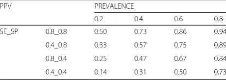
For instance, with a high SE of 0.9, a SP of 0.4 and a prevalence of 0.30, the PPV is 0.4. There is a 40% chance of presence of the clinical condition with a positive test. In contrast to the high sensitivity, this is quite confront-ing. Another example: The prevalence of SLAP lesions has been reported between 6 and 26% [7]. For the O’Brien test (used to detect a SLAP lesion), taking into account the pooled results for SE and SP of respectively 0.66 and 0.36, PPV would range between 6% (for a prevalence of 6%) and 27% (for a prevalence of 26%) [8].

prevalence on the PPV values. The table also demon-strates that the PPV is not uniquely related to the SE but on the combination of SE and SP. For instance, the combination of a low SE and high SP (0.4_0.8) presents higher PPV values than the combination of a high SE and low SP (0.8_0.4).

Initiated by Sacket et al. [9] it is commonly believed that if a very high SP is present the SPIN rule can be of use. SPIN is the acronym for‘Specific test when Positive rules IN the disease’. The rationale behind the SPIN rule is that a test with a high SP is very specific with what it tests for, it is good at excluding the clinical condition. So, if the test has a high SP and the result is positive one can be nearly certain that the clinical condition is present.

The SPIN rule is a statement from the point of view of the conditional statement P(1∖+ )= PPV.

SPIN relates a high SP to an acceptable PPV. However, as can be seen in Table 2, the ability to rule in depends not only on the SP but also on the SE AND the preva-lence. Consequently, the SPIN rule is not applicable when the prevalence is low. Furthermore, the PPV is re-duced when a high SP is combined with a low SE (for instance PPV = 0.57 under a prevalence of 0.4 for SE_SP 0.4_0.8 as compared to PPV = 0.73 for SE_SP 0.8_0.8 under same prevalence of 0.4).

The same reasoning can be applied on the statement P(0∖ −),i.e. ‘What is the chance that the clinical event will not be present (0) when a negative test (-) result is present?’Given the probability P(0) as the proportion of

healthy people for the target disorder (i.e. P(0) = 1 – prevalence = 1–P [1], = n_n0), and P(−) the probability of a clinical index test being negative (i.e. h

n). Then Pð0∖−Þ ¼Pð0∩−Þ

Pð−Þ ¼ h0=n

h=n ¼ h0

h ¼NPV and Pð−∖0Þ ¼ Pð0∩−Þ

Pð−Þ ¼ h0=n n0=n ¼h0

h0¼SP . Here also, P(−∖0) ≠P(0∖ −)! As well as the PPV, the NPV is dependent on the prevalence P [1], the SE and the SP of the test:

NPV¼ ð1−PREVALENCEÞ specificity

PREVALENCEð1−sensitivityÞ þð1−PREVALENCEÞ specificity

¼ ð1−Pð Þ1Þ SP Pð Þ 1 ð1−SEÞ þð1−Pð Þ1Þ SP

1-NPV is termed the ‘POST- test probability of a NEGATIVE test’.

For example: For the O’Brien test, taking into account the pooled results for SE and SP of respectively 0.66 and 0.36, NPV would range between 94% (for a prevalence of 6%) and 75% (for a prevalence of 26%) [4]. Two pecu-liar things are presented here: the bigger the prevalence the smaller the NPV and despite a small SP, the NPV is relatively larger. This needs clarification.

Table 3 presents a Monte Carlo simulation for NPV related to differences in prevalence (P [1]), SE and SP, categorized in four combinations of SE and SP (0.8_0.8; 0.8_0.4; 0.4_0.8; 0.4_0.4) and four levels of prevalence (0.2, 0.4, 0.6, 0.8). The table reveals the impact of the prevalence on the NPV values, but opposite to the PPV NPV decreases with an increase in prevalence. The table also demonstrates that the NPV is not uniquely related to the SE but merely on the combination of SE and SP. For instance, the combination of a low SE and high SP (0.4_0.8) presents higher NPV values than the combin-ation of a high SE and low SP (0.8_0.4), which is oppos-ite to the finding for PPV (as mentioned above).

SNOUT is the acronym for‘Sensitive test when Nega-tive rules OUT the disease’[9]. The rationale behind the SNOUT rule is that if a test has a high sensitivity, one can be confident that it will detect the clinical event and so if the test result is negative, one can be nearly certain that the clinical condition is not present. The SNOUT rule is actually a statement from the point of view of the conditional statement P(0∖-) = NPV. SNOUT intrinsic-ally relates a high SE to an acceptable NPV. From the

Table 2PPV values in relation to prevalence, SE and SP values SE_SP = value of SE _ values of SP

PPV PREVALENCE

0.2 0.4 0.6 0.8

SE_SP 0.8_0.8 0.50 0.73 0.86 0.94

0.4_0.8 0.33 0.57 0.75 0.89

0.8_0.4 0.25 0.47 0.67 0.84

0.4_0.4 0.14 0.31 0.50 0.73

Table 3NPV values in relation to prevalence, SE and SP values SE_SP = value of SE _ values of SP

NPV PREVALENCE

0.2 0.4 0.6 0.8

SE_SP 0.8_0.8 0.94 0.86 0.73 0.50

0.4_0.8 0.84 0.67 0.47 0.25

0.8_0.4 0.89 0.75 0.57 0.33

0.4_0.4 0.73 0.50 0.31 0.14

Table 1Contingency table between a clinical condition and clinical index test result

Test result Cinical condition 1 0

+ d1 d0 d = n+

– h1 h0 h = n−

n1 n0 n

‘True positives’= d1 = the patient has the clinical condition[1]and the clinical test is positive (+)

‘False positives’= d0 = the patient does not have the clinical condition (0) but the clinical test is positive (+)

‘True negatives’= h0 = the patient does not have the clinical condition (0) and the clinical test is negative (−)

‘False negatives’= h1 = the patient has the clinical condition[1]and the clinical test is negative (−)

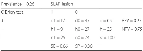
table, it is clear that this is only applicable for the lower prevalences. Furthermore, a low SE can also be associ-ated to an acceptable NPV under the condition of low prevalence. Consequently, the SNOUT rule can be very misguiding within the diagnostic process. Considering the abovementioned arguments, the use of SE and SP should be avoided in clinical diagnosis because it is re-lated to a wrong point of view, namelyP(+∖1) orP(−∖0). Also SPIN and SNOUT should be avoided due to its condi-tional limitations related to prevalence and combination of SP and SE. PPV and NPV are related to the right point of view for clinical diagnosis, namelyP(1∖+) orP(0∖−). When considering predictive values of diagnostic tests, one must however, recognise and accentuate the influence of the prevalence of the clinical event. Whereas the weakness of SE and SP is their relationships to the conditional state-ments P(+∖1) and P(−∖0),the problem with PPV and NPV is that they are predictive values largely dependent on the prior probability. Consequently, predictive values from one study should not be transferred to some other setting with different prevalences. Prevalence affects PPV and NPV dif-ferently. PPV is increasing, while NPV decreases with the in-crease of the prevalence. When the prevalence is very high, a negative test is most likely a false negative. When preva-lence is very low, a positive test is most likely a false positive. Predictive values have a clear meaning in clinical con-text. If a patient is tested positive with the O’Brien test for a SLAP lesion, the patient may ask:‘Does this mean I have this clinical condition?’. ‘No’you answer,‘it is not certain for 100%. The patient ‘I understand that it is not totally clear, but what then is the chance that I have this prob-lem?’Given 26% as the highest prevalence presented in lit-erature for a SLAP lesion and given a pooled estimate for SE of 0,66 and for SP 0,36, PPV is 0,27 and NPV is 0,75 (the contingency table is presented in Table4).

You answer the patient:‘In 100 persons presenting posi-tively on the test, 30 of them will have the clinical condi-tion. What then is the ‘negative predictive value’? This is 0.8, whereby with a negative test result there is a 20% chance of presence of the clinical condition, which is also called the post-test probability of a negative test’(1–0.8).

Because the PPV and NPV are dependent on the pre-test probability, these scores are termed post-test probabilities. At first sight, the PPV and NPV are measures which re-spond to the clinical relevant question:‘what is the chance that the clinical condition will be present or absent in con-text of a positive or negative test result?’. However, the in-terpretation of the PPV and NPV is limited to populations with the same prevalence of clinical condition as the spe-cific population to which the patient belongs. The preva-lence in a clinical setting may differ considerably between for instance primary care practice and hospital. Patients in primary care practice will generally have the clinical condi-tion at an earlier and milder stage.

Due to its influence and unknown differences between clinical settings, prevalence is the nemesis in the application of the predictive values. Therefore, another variable has been introduced to evaluate the strength of a diagnostic test, namely the likelihood ratio. Likelihood ratios deter-mine how much more likely a particular test result is among people who have the clinical condition of interest than it is among people who do not have the condition. LIKELIHOOD RATIO (LR) is the ratio of two probabilities. The positive likelihood ratio (LR+) is the ratio between the proportion of the individuals having the clinical sta-tus and presenting a positive test result to the propor-tion of the individuals not having the clinical condipropor-tion but presenting with a positive test result: POSITIVE

LIKELIHOOD RATIO = LR+ = P_Pðþ_ðþ∖_∖1₀Þ_Þ=

d1.

n1

d0

n0 .

A positive likelihood ratio is a measure of how much more likely a positive test result is among people who have the condition of interest than it is among people who do not have the condition of interest. For instance, with the data presented in Table4, LR+ = 1.03, meaning that the likelihood of a positive outcome of the O’Brien test in patients with a SLAP lesion is only 3% higher than in patients without SLAP lesions.

The negative likelihood ratio (LR-) is the ratio between the proportion of the individuals having the clinical sta-tus and presenting a negative result on the clinical test to the proportion of the individuals not having the clin-ical condition and presenting with a negative test result:

NEGATIVE LIKELIHOOD RATIO¼LR−P_Pð_ð−∖_−∖1₀Þ_Þ¼ h1.

n1 h0

n0 .

A negative likelihood ratio is a measure of how much more likely a negative test result is among people who have the condition of interest than it is among people who do not have the condition of interest.

With SE¼d1

n1 and SP¼hn00¼n0n−d00 it can be deduced that d0

n0¼1−SP . This gives for LRþ ¼1SE−SP and analo-gously for LR−¼1−SE

SP . LR+ is related to the concept

‘ruling IN the disease’, LR- to ‘ruling OUT the disease’. Likelihood ratios of 1 indicate that the test is uninformative.

Table 4Contingency table for the O’Brien test with a SE of 0.66 and SP of 0.36 under prevalence of 0.26

Prevalence = 0.26 SLAP lesion

O’Brien test 1 0

+ d1 = 17 d0 = 47 d = 65 PPV = 0.27

– h1 = 9 h0 = 27 h = 35 NPV = 0.75

n1 = 26 n0 = 74 n= 100

A LR+ bigger than 1 means that the probability for presence of the clinical entity is more than chance (head or tail). A LR- smaller than 1 means that the probability of absence of the clinical entity is bigger than head or tail chance. LR+ ranges from 1 to infinity, LR- from 0 to 1. LRs have a strong power because LR+ and LR- are in-dependent of the prevalence in the population. Likeli-hood ratios have a number of potencies. First, LRs can be combined with the pre-test probability to calculate the post-test predictive values PPV and NPV using for-mulas based on Bayes’s theorem [10]:

With λ¼

prevalence

ð1−prevalenceÞLR

prevalence

ð1−prevalenceÞLRþ1

, PPV =λ (with LR = LR+) and

NPV = 1- λ (with LR = LR-). Furthermore, LRs are applic-able in populations in which the clinical condition may have a different prevalence to the population from which the likelihood ratio was calculated.

With a likelihood ratio nomogram post-test, probabil-ities can be deduced from the pre-test probability and the LR [10].

To avoid the calculations to find the shift from prior probability) to posterior probability (PVs), McGee (2002) described a simpler method (under the condition of prevalence between 10 and 90%) to interpret LRs using (so called ‘bedside’) estimates of approximate change in probability of the clinical event (in %) accurate to within 10% for a prevalence between 10 and 90% [11].

A LR+ bigger than 10, indicating an estimated shift in probability of at least 45%, has been stated to be strongly indicative for the presence of a clinical entity, between 5 and 10 moderate (estimated shift of at least 30%) and between 2 and 5 weak (estimated shift 15%) [10, 11]. A LR- less than 0.1 is strongly indicative for absence of the

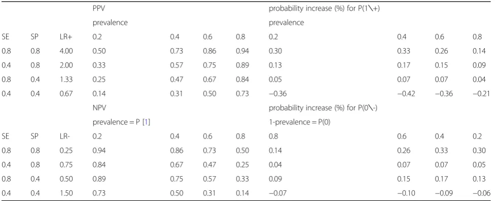
clinical entity (estimated shift at least 45%), between 0.1 and 0.2 moderate (estimated shift at least 30%) and be-tween 0.2 and 0.5 weak (estimated shift at least 15%) [10]. However, in musculoskeletal disorders, the LRs hardly approach a maximum of 4 for LR+ and 0.25 for LR−. For instance, in their recent meta-analysis on phys-ical examination tests of the shoulder, Gismervik et al. (2017) presented pooled results of LR+s ranging between 0.67 and 3.91 (with those being bigger than 1 between 1.03 and 3.91). LR−s ranged between 0.63 and 1.06 (with those smaller than 1 between 0.57 and 0.91) [4]. Table5 presents the increase in probability (i.e. posterior prob-ability –prior probability = posttest probability – preva-lence) as related to a Monte Carlo representation of combinations between SE and SP. To accentuate is the decrease in probability under the condition of SE 0.4 and SP 0.4 for the LR+ as well as for the LR-.

To return to our patient who tested positive on the O’Brien’s test. With a prevalence of 026, a SE of 0.66 and a SP of 0.36, the LR+ of the O’Brien test is only 1.03, i.e. very weak. The test increases the prior probability (preva-lence) of 0.26 up to a posterior probability (PPV) of 0.27, an increase of only 1%, And with the prior probability P(0) of 0.8 reduced to a NPV of 0.75, this makes the O’Brien test worthless under the condition of the 0.26 prevalence. To be sure, you need to advice the patient to proceed with other investigations (medical imaging).

As stated above, the main nemesis in clinical diagnosis is the pre-test probability (prevalence). This must not be restricted to the prevalence of the clinical event in the population. Based on the anamnestic information, the physiotherapist may think of a particular clinical prob-lem (primary hypothesis) in varying degrees of likeliness. Table 5Probability increases (%) for P(1∖+) and for P(0∖-) in relation to prevalence and LRs

PPV probability increase (%) for P(1∖+)

prevalence prevalence

SE SP LR+ 0.2 0.4 0.6 0.8 0.2 0.4 0.6 0.8

0.8 0.8 4.00 0.50 0.73 0.86 0.94 0.30 0.33 0.26 0.14

0.4 0.8 2.00 0.33 0.57 0.75 0.89 0.13 0.17 0.15 0.09

0.8 0.4 1.33 0.25 0.47 0.67 0.84 0.05 0.07 0.07 0.04

0.4 0.4 0.67 0.14 0.31 0.50 0.73 −0.36 −0.42 −0.36 −0.21

NPV probability increase (%) for P(0∖-)

prevalence = P [1] 1-prevalence = P(0)

SE SP LR- 0.2 0.4 0.6 0.8 0.8 0.6 0.4 0.2

0.8 0.8 0.25 0.94 0.86 0.73 0.50 0.14 0.26 0.33 0.30

0.4 0.8 0.75 0.84 0.67 0.47 0.25 0.04 0.07 0.07 0.05

0.8 0.4 0.50 0.89 0.75 0.57 0.33 0.09 0.15 0.17 0.13

0.4 0.4 1.50 0.73 0.50 0.31 0.14 −0.07 −0.10 −0.09 −0.06

Standard screening and red flags questions may have ruled out specific conditions. Once the primary hy-pothesis of clinical condition is expressed, a conscious levelling of the prior probability of this condition can be made.

Take home messages

Therapists should not rely on the SNOUT and SPIN mnemomics.

Prevalence is the nemesis in diagnosis but can be ‘upgraded’based on anamnesis and the levelling of a prior probability.

PPV and NPV are dependent on SE, SP and prevalence.

Withλ=

prevalence ð1−prevalenceÞLR prevalence ð1−prevalenceÞLRþ1

, the best approach is to use

the LRs in combination with a prevalence estimation to calculate the PPV (PPV=PV) and NPV (NPV = 1-PV) [10].

Abbreviations

∩:Boolean operator‘and‘; DA: Diagnostic accuracy; FNF: True Negative Fraction; FPF: False Positive Fraction; LR: Likelihood ratio; NPV: Negative Predictive Value; P: Probability; PPV: Positive predictive value; PV: Post test probability; SE: Sensitivity; SLAP: Superior labrum anterior and posterior; SNOUT: Sensitive test when Negative rules OUT the disease; SP: Specificity; SPIN: Specific test when Positive rules IN the disease; TNF: True negative fraction; TPF: True positive fraction

Acknowledgements

The authors thank the Thim van der Laan Foundation, Switzerland for the support.

Funding No funding.

Availability of data and materials

Data sharing is not applicable to this article as no datasets were generated or analysed during the current study.

Authors’contributions

Each author has participated and contributed sufficiently to take public responsibility for appropriate portions of the content. JPB conceived the original manuscript. BS and MG drafted the tables and statistical formula. RC carried out the literature review and drafted the manuscript. JPB, BS, MG and RC were involved in the critical revision and development of the manuscript. All authors read and approved the final manuscript.

Authors_’information Prof dr Baeyens Jean-Pierre,

laboratory Biomechanics_–Vrije Universiteit Brussel

studies: revalidation sciences, biomedical sciences, art history & archeology lectures: biomechanics and statistics biomechanics

research projects: overhand sports biomechanics, repetitive strain injuries in musicians, stress urinary incontinence, cerebral palsy

Ethics approval and consent to participate

“Not applicable”.

Consent for publication

“Not applicable”.

Competing interests

Author RC is a member of the editorial board of the journal. The authors declare that they have no competing interests.

Publisher’s Note

Springer Nature remains neutral with regard to jurisdictional claims in published maps and institutional affiliations.

Author details

1_{Faculty Physical Education and Physiotherapy, Vrije Universiteit Brussel,}

Pleinlaan 2, 1050 Brussel, Belgium.2_{International University of Applied}

Sciences THIM, Weststrasse 8, 7302 Landquart, Switzerland.3Faculty Applied Engineering, Antwerp University, Campus Groenenborgerlaan 171, G.U. 148, 2020 Antwerpen, Belgium.4_{Department of Business Economics, Health and}

Social Care, SUPSI, Weststrasse 8, 7302 Landquart, Switzerland.

Received: 14 October 2018 Accepted: 8 February 2019

References

1. Jutel A. Sociology of diagnosis: a preliminary review. Sociol Health Illn. 2009; 31(2):278_–99.

2. Rutjes AW, Reitsma JB, Coomarasamy A, Khan KS, Bossuyt PM. Evaluation of diagnostic tests when there is no gold standard. A review of methods. Health Technol Assess. 2007;11(50):iii):ix–51.

3. Sackett DL, Haynes RB. Architecture of diagnostic research. BMJ. 2002; 324(7336):539–41.

4. Gismervik SO, Drogset JO, Granviken F, Ro M, Leivseth G. Physical examination tests of the shoulder: a systematic review and meta-analysis of diagnostic test performance. BMC Musculoskelet Disord. 2017;18(1):41. 5. Ransohoff DF, Feinstein AR. Problems of spectrum and bias in evaluating

the efficacy of diagnostic tests. N Engl J Med. 1978;299(17):926–30. 6. Whiting PF, Rutjes AW, Westwood ME, Mallett S, Group Q-S. A systematic

review classifies sources of bias and variation in diagnostic test accuracy studies. J Clin Epidemiol. 2013;66(10):1093–104.

7. Erickson BJ, Jain A, Abrams GD, Nicholson GP, Cole BJ, Romeo AA, et al. SLAP lesions: trends in treatment. Arthroscopy. 2016;32(6):976–81. 8. O'Brien SJ, Pagnani MJ, Fealy S, McGlynn SR, Wilson JB. The active

compression test: a new and effective test for diagnosing labral tears and acromioclavicular joint abnormality. Am J Sports Med. 1998;26(5):610–3. 9. Sackett DL, Straus S. On some clinically useful measures of the accuracy of

diagnostic tests. ACP J Club. 1998;129(2):A17_–9.

10. Fagan TJ. Letter: Nomogram for Bayes theorem. N Engl J Med. 1975;293(5):257. 11. McGee S. Simplifying likelihood ratios. J Gen Intern Med. 2002;17(8):646–9. 12. MedCalc’s Diagnostic test evaluation calculator.https://www.medcalc.org/

calc/diagnostic_test.phpAccessed 29 August 2018.