R E S E A R C H
Open Access
Iterative methods for ternary diffusions
Henryk Leszczy ´nski
*and Monika Wrzosek
*Correspondence:
Institute of Mathematics, University of Gda ´nsk, Wita Stwosza 57, Gda ´nsk, 80-952, Poland
Abstract
We apply iterative methods to three-component diffusion equations and study their convergence inL2and in the Sobolev spaceW1,∞. The system is parabolic and
mass-conservative. Newton’s method converges very fast and its iterations do not leave the set of admissible functions.
MSC: 35K51; 35K57; 65M12; 65M80
Keywords: diffusion; iterative method; Newton’s method
1 Introduction
Since its discovery and later analysis by Darken [], the Kirkendall effect [] has been found in various alloy systems, and studies on lattice defects and diffusion developed signifi-cantly. The Danielewski-Holly method [] extends the Darken standard theory of interdif-fusion and describes the process in the bounded mixture showing constant concentration. Under certain regularity assumptions and quantitative condition Danielewski and Holly proved the existence and uniqueness of solution to PDE describing the interdiffusion phe-nomena. Further developments have been presented in numerous articles;e.g.[, ].
In the paper we apply Newton’s method (see [–]) to three-component diffusion equa-tions and study the convergence inLand Sobolev spaceW,∞. The system of equations
is strongly coupled, however, the maximum principle presented in Section confirms its parabolic type. Parabolicity is additionally confirmed by our convergence result for itera-tive methods. This falsifies the nonparabolicity hypothesis by Danielewski and Holly [], where they construct an initial concentration whoseL norm increases in time, at least
on some interval. The Newton method, known asquasilinearization method, is very use-ful in modern numerical methods for solving PDE’s; see []. We apply this method to strongly coupled parabolic systems describing diffusing mixtures. This strong parabol-icity might have caused weird phenomena, but we have discovered a kind of maximum principle and some conservation laws in this system, hence the iterative methods pro-posed here behave very well. Our result is very useful in numerical simulations when one wants to construct reliable and fast convergent approximations. Since Newton’s method produces linear PDE’s satisfying maximum principles anda prioriestimates of the respec-tive Green functions or Cauchy kernels, one can find errors estimates much better than those obtained from the Newton-Kantorovich theorem, cf. [, ].
Consider a mixture composed of three different components. Let t≥,x∈[–L,L],
vi: [,∞)×[–L,L]→Rdenote the velocity field of theith component andci: [,∞)× [–L,L]→Rits molar density or molar concentration. It is a measure of the number of
particles contained in any volume,c+c+c≡const. The component diffusion flux is a
Fickian flow:
Jid(t,x) := –Digradci,
where Di is the intrinsic diffusitivity of theith component which we assume to satisfy
D>D>D> . DenoteDi:=Di–Dfori= , . The overallith component flux is a sum
of diffusion and convection fluxes:
Ji:=Jid+civD,
wherevDstands for a drift velocity. By the mass conservation law:
∂ci
∂t = –divJi
and upon denotingu=c,v=c,w=cwe arrive at the following system of equations:
ut=Duxx–
uDux+Dvx
x,
vt=Dvxx–
vDux+Dvx
x,
wt=Dwxx–
wDux+Dvx
x
(.)
with the initial condition
u(,x) =u(x), v(,x) =v(x), w(,x) =w(x) = –u(x) –v(x) (.)
forx∈[–L,L] and the Neumann boundary condition
∂u ∂n= ,
∂v ∂n= ,
∂w
∂n = fort≥,x∈ {–L,L}. (.)
LetXdenote the space consisting of triples of functions (u,v,w) satisfying
u,v,w∈C,,
ux,uxx,vx,vxxare bounded,
u≥,v≥,w≥fort≥,x∈[–L,L], u+v+w= fort≥,x∈[–L,L],
u,v,wobey the Neumann boundary condition.
Remark . If (u,v,w)∈Xthen the third equation of (.) is not necessary, sincew= –
u–v. However, we keep it for a more convenient analysis of some properties of solutions.
Remark . We call
vD=Dux+Dvx=Dux+Dvx+Dwx
Lemma .(Mass conservation) If(u,v,w)∈X satisfy(.), (.)then
L
–L
u dx=const.,
L
–L
v dx=const.,
L
–L
w dx=const.
Proof The relation
d dt
L
–L
u dx=
can be shown by means of the Neumann boundary condition.
Lemma .(Maximum principle) Suppose that u(,·),v(,·),w(,·)∈Cand
u(,x)≥, v(,x)≥, w(,x)≥, u(,x) +v(,x) +w(,x) =
for x∈[–L,L].If(u,v,w)satisfy(.)-(.)then(u,v,w)∈X.
Proof Letu˜=u+εeλt,v˜=v+εeλt,w˜ =w+εeλtforε> . We have
˜
ut=ut+ελeλt, u˜x=ux, u˜xx=uxx,
˜
vt=vt+ελeλt, v˜x=vx, v˜xx=vxx.
There existsλ∈R(sufficiently large) such that we have strong differential inequalities:
˜
ut>Du˜xx–u˜
Du˜xx+Dv˜xx
–u˜x
Du˜x+Dv˜x
,
˜
vt>Dv˜xx–v˜
Du˜xx+Dv˜xx
–˜vx
Du˜x+Dv˜x
,
˜
wt>Dw˜xx–w˜
Du˜xx+Dv˜xx
–w˜x
Du˜x+Dv˜x
.
We claim that u˜ > ,v˜> , w˜ > in the whole domain. Suppose that this is not true and take the smallest t∗> such that u˜(t∗,x∗) = , orv˜(t∗,x∗) = , orw˜(t∗,x∗) = for some x∗ ∈[–L,L]. Without loss of generality we assumeu˜(t∗,x∗) = . Sinceu˜(t∗,x∗) =
min{t≤t∗,x∈[–L,L]}u˜(t,x) we haveu˜x(t∗,x∗) = ,u˜t(t∗,x∗)≤ andu˜xx(t∗,x∗)≥. Hence
≥ ˜ut
t∗,x∗>Du˜xx
t∗,x∗–u˜t∗,x∗Du˜xx
t∗,x∗+Dv˜xx
t∗,x∗
–u˜x
t∗,x∗Du˜x
t∗,x∗+Dv˜x
t∗,x∗≥,
which is a contradiction. Thusu˜> fort≥,x∈[–L,L]. Ifε→+thenu˜→u. Hence
u> . Similarly,v(t,x)≥ andw(t,x)≥ fort≥,x∈[–L,L].
2 Uniqueness
LetX¯ be the closure ofX w.r.t. theLnorm. The existence and uniqueness of solutions
to problem (.)-(.) inX w.r.t. the Sobolev normW, is given in []. The following
proposition concerns the uniqueness of solutions inL. Since the set ofC-functions is
Proposition . Assume that( – √)D≤D≤( +
√
)Dand(u,v,w)∈ ¯X.Then
a weak solution(u,v,w)∈ ¯X to problem(.)-(.)is unique in L.
Proof Since everyL-function can be approximated by a sequence of X-functions, it
suffices to show the uniqueness ofX-solutions w.r.t. theL-norm. Let (u,v,w)∈X and
(u¯,v¯,w¯)∈Xbe solutions to (.)-(.). Denote
u=u–u¯, v=v–v¯, w=w–w¯
and observe that
ut=Duxx–
uDux+Dvx
x–
¯
uDux+Dvx
x,
vt=Dvxx–
vDux+Dvx
x–
¯
vDux+Dvx
x,
wt=Dwxx–
wDux+Dvx
x–
¯
wDux+Dvx
x.
We have
L
–L
uutdx=D L
–L
uuxxdx–
L
–L
uuDux+Dvx
xdx
–
L
–L
uu¯Dux+Dvx
xdx.
Using integration by parts we obtain
D L
–L
uuxxdx= –D L
–L
(ux)dx,
L
–L
uuDux+Dvx
xdx=
L
–L
(u)Duxx+Dvxx
dx,
L
–L
uu¯Dux+Dvx
xdx= –
L
–L uxu¯
Dux+Dvx
dx. Hence d dt L –L
(u)+ (v)+ (w)dx
=
L
–L
(uut+vvt+wwt)dx
= –
L
–L
D(ux)+D(vx)+D(wx) dx – L –L
(u)+ (v)+ (w)Duxx+Dvxx
dx
+
L
–L
(uxu¯+vx¯v+wxw¯)
Dux+Dvx
By the fact thatwx= –ux–vxwe obtain
L
–L
(uut+vvt+wwt)dx
= –
L
–L
(u)+ (v)+ (w)Duxx+Dvxx
dx
–
L
–L
D+D–D(u¯–w¯)
(ux)dx
–
L
–L
D+D–D(v¯–w¯)
(vx)dx
–
L
–L
D–D(¯v–w¯) –D(u¯–w¯)
uxvxdx.
We examine the nonnegative definiteness of the matrix:
A=
D+D–D(u¯–w¯) D–D(v¯–w¯) –D(u¯–w¯)
D–D(¯v–w¯) – D(u¯–w¯) D+D–D(¯v–w¯)
i.e.
D+D–D(u¯–w¯)≥, D+D–D(¯v–w¯)≥, and det(A)≥.
The first two inequalities are true due to the relations:
–≤ ¯u–w¯≤, –≤ ¯v–w¯ ≤, D>D>D> .
The condition
( – √)D≤D≤( +
√ )D
impliesdet(A)≥ for all admissibleu¯,w¯.
3 Iterative methods
Recall that
Dux+Dvx=Dux+Dvx+Dwx,
Duxx+Dvxx=Duxx+Dvxx+Dwxx.
Assume that (u(),v(),w()) coincides with (u,v,w) att= and formulate an iterative
method for (.)-(.):
u(tk+)=Du(xxk+)–
u(k)Du(xk+)+Dv(xk+)+Dw(xk+)
x,
v(tk+)=Dv(xxk+)–
v(k)Du(xk+)+Dv(xk+)+Dw(xk+)
x,
w(tk+)=Dw(xxk+)–
w(k)Du(xk+)+Dv(xk+)+Dw(xk+)
x,
with the initial condition
u(k+)(,x) =u(x), v(k+)(,x) =v(x), w(k+)(,x) =w(x) (.)
forx∈[–L,L] and the Neumann boundary condition. Moreover, assume that
u(x) +v(x) +w(x) = (.)
forx∈[–L,L]. Denote
u(k)=u(k+)–u(k), v(k)=v(k+)–v(k), w(k)=w(k+)–w(k).
Lemma . Assume u,v,w∈X, (u(),v(),w()) = (u,v,w)at t= and u()+v()+
w() = .If(u(k),v(k),w(k))fulfills(.)with(.), the Neumann boundary condition and
(.),then u(k)+v(k)+w(k)= .
Proof It suffices to showu(k)+v(k)+w(k)= ⇒u(k+)+v(k+)+w(k+)= . We assume the
induction hypothesisu(k)+v(k)+w(k)= . Thus
ut(k+)+vt(k+)+w(tk+)
=Du(xxk+)+Dvxx(k+)+Dw(xxk+)
–u(xk)+vx(k)+w(xk)Dux(k+)+Dvx(k+)+Dw(xk+)
–u(k)+v(k)+w(k)Duxx(k+)+Dvxx(k+)+Dw(xxk+)
≡.
Hence the statement is proved.
The following theorem establishes a convergence of the iterative method (.)-(.).
Theorem . Suppose(u,v,w)∈Xand(u(),v(),w()) = (u,v,w)at t= .If u(xk),v(xk),
w(xk)are Cand
≤u(k)≤, ≤v(k)≤, ≤w(k)≤ for k= , , . . .
then the sequence(u(k),v(k),w(k))defined by(.), (.)converges to the solution(u,v,w)of
(.), (.)in the Sobolev space W,∞.
Proof As in the previous section denote the incrementsu(k)=u(k+)–u(k),v(k)=v(k+)–
v(k),w(k)=w(k+)–w(k). From (.) we have the following differential equations:
u(tk+)=Du(xxk+)–
u(k+)Dux(k+)+Dv(xk+)x
–u(k)Dux(k+)+Dv(xk+)x,
v(tk+)=Dv(xxk+)–
v(k+)Dux(k+)+Dv(xk+)x
–v(k)Du(xk+)+Dv(xk+)+Dw(xk+)
Using the Green functionsG,k,G,kcorresponding to the differential operators
∂ ∂t–D
∂
∂x +u(k+)D ∂
∂x D ∂ ∂x
D∂
∂x ∂∂t–D∂
∂x +v(k+)D∂ ∂x
(.)
we have
u(k+)(t,x)
v(k+)(t,x) = t L –L
G,k(t,s,x,y)P,k(s,y)
G,k(t,s,x,y)P,k(s,y)
dy ds,
u(xk+)(t,x) v(xk+)(t,x)
= t L –L
G,k
x (t,s,x,y)P,k(s,y)
G,k
x (t,s,x,y)P,k(s,y)
dy ds,
wherePi,k(s,y) depend onu(k),v(k),u(k)
x ,v(xk),ux(k+),v(xk+)fori= , . The Green functionsGi,kdepend onu(k),v(k)and have the uniform estimates
L
–L
Gi,k(t,s,x,y) dy≤C,
L
–L
Gxi,k(t,s,x,y) dy≤√C
t–s, (.)
with some generic constantCnot depending onk. By Lemma . there existsM≥ such that
u(xk+)(t,·)L∞≤M, v(xk+)(t,·)L∞≤M,
u(xxk+)(t,·)L∞≤M, v(xxk+)(t,·)L∞≤M.
(.)
Since
P,k(t,·)L∞≤M
D+Du(k)(t,·)L∞+M
D+Dux(k)(t,·)L∞
+MDux(k+)(t,·)L∞+MDvx(k+)(t,·)L∞
we get
u(k+),v(k+)(t,·)W,∞:=u(k+)(t,·)W,∞+v(k+)(t,·)W,∞
≤
t
C
√
t–su
(k),v(k)(s,·)
W,∞ds
+
t
C
√
t–su
(k+),v(k+)(s,·)
W,∞ds.
Applying Lemma A. we have(u(),v())(t,·)W
,∞≤Kand by induction: (u(k),
v(k))(t,·)W,∞≤K
kt
k
fork= , , . . . . Hence
Kk+=Kk
C
– CT/
θk √
–θdθ.
Notice that
Kk+
Kk
= C
– CT/
θk √
–θdθ→ ask→ ∞.
We give sufficient conditions for the successive approximations to remain inX.
Proposition . Assume that u,v∈C, <ε≤u(x)≤ –ε< , <ε≤v(x)≤
–ε< and the sequence(u(k),v(k),w(k))defined by(.)with the first element given by
u()(t,x) =u(x) +tku(x) and v()(t,x) =v(x) +tkv(x),
where ku,kv∈Xare of the form
ku(x) =Du(x) –
u(x)
Du(x) +Dv(x)x,
kv(x) =Dv(x) –
v(x)
Du(x) +Dv(x)x,
converges to the solution(u,v,w)of (.), (.)in the Sobolev space W,∞.If
∞
k=
Kktk/≤ε, where Kk=Kk–
C
– CT/
θk– √
–θdθ,
then≤u(k)(t,x)≤and≤v(k)(t,x)≤,k= , , . . . .
Proof We have
u()t (t,x) =ku(x), u()x (t,x) =u(x) +tku(x), u()xx(t,x) =u(x) +tku(x).
Hence
ku(x) =Du(x) –u(x)
Du(x) +Dv(x)–u(x)
Du(x) +Dv(x)
=D
u()xx(t,x) –tku(x)
–u()x (t,x) –tku(x)Du()x +Dv()x –tDku(x) +Dkv(x)
–u()(t,x) –tku(x)Du()xx +Dv()xx–tDku(x) +Dkv(x).
Thus we get
u()t (t,x) =u()t (t,x) –u()t (t,x)
=Du()xx(t,x) –u()x (t,x)
Du()x (t,x) +Dv()x (t,x)
–u()(t,x)Du()xx(t,x) +Dv()xx(t,x)–ku(x)
=Du()xx(t,x) –
u()(t,x)Du()x (t,x) +Dv()x (t,x)x
+tR(x) +tR(x),
where
R(x) :=Dku(x) –u()x (t,x)
Dku(x) +Dkv(x)–ku(x)Du()x (t,x) +Dv()x (t,x)
–u()(t,x)Dku(x) +Dkv(x)–ku(x)Du()xx(t,x) +Dv()xx(t,x),
R(x) :=ku(x)
For ≤t≤Twe have
RL∞=tR+tRL∞≤T
RL∞+TRL∞
=:K.
Thus
u(),v()(t,·)W,∞≤
t
C
√
t–su
(),v()(s,·)
W,∞+K
ds.
Applying Lemma A. we have
u(),v()(t,·)W,∞≤Kt/
and by induction(u(k),v(k))(t,·)W
,∞≤Kk+t k+
fork= , , . . . . Hence
Kk+=Kk
C
– CT/
θk √
–θdθ.
Remark . The functionsku,kv∈Xcan be slightly perturbed near the lateral boundary in order to fulfill the Neumann boundary condition.
4 Convergence of the Newton method
As in the previous section denote
u(k)=u(k+)–u(k), v(k)=v(k+)–v(k), w(k)=w(k+)–w(k).
We assume that (u(),v(),w()) = (u
,v,w) att= and formulate the Newton method
for (.)-(.):
u(tk+)=Du(xxk+)–
u(k)Dux(k)+Dv(xk)x
–u(k)Dux(k)+Dv(xk)x–u(k)Dux(k)+Dv(xk)x,
v(tk+)=Dv(xxk+)–
v(k)Dux(k)+Dv(xk)x
–v(k)Dux(k)+Dv(xk)x–v(k)Dux(k)+Dv(xk)x,
w(tk+)=Dw(xxk+)–
w(k)Dux(k)+Dv(xk)x
–w(k)Dux(k)+Dv(xk)x–w(k)Dux(k)+Dv(xk)x,
(.)
with the initial condition (.) and the Neumann boundary condition.
Lemma . Assume u,v,w∈X, (u(),v(),w()) = (u,v,w)at t= and u()+v()+
w() = .If(u(k),v(k),w(k))fulfills(.)with(.)and the Neumann boundary condition,
Proof We showu(k)+v(k)+w(k)= ⇒u(k+)+v(k+)+w(k+)= . The only solution to the
differential equation
u(tk+)+v
(k+)
t +w
(k+)
t
= –u(xk+)+vx(k+)+w(xk+)Dux(k)+Dvx(k)+Dw(xk)
–u(k+)+v(k+)+w(k+)– Du(xxk)+Dvxx(k)+Dw(xxk)
isu(k+)+v(k+)+w(k+)≡.
The following theorem establishes the convergence of the Newton method.
Theorem . Suppose(u,v,w)∈Xand(u(),v(),w()) = (u,v,w)at t= .If u(xk),v(xk),
w(xk)are Cand
≤u(k)≤, ≤v(k)≤, ≤w(k)≤ for k= , , . . . ,
then the sequence(u(k),v(k),w(k))defined by(.), (.)converges to the solution(u,v,w)of
(.)-(.)with respect to the norms in the Sobolev space W,∞.
Proof We have the following differential equations:
u(tk+)=Du(xxk+)–
u(k)Dux(k)+Dv(xk)x
–u(k+)Dux(k+)+Dv(xk+)x–u(k+)Dux(k+)+Dv(xk+)x,
v(tk+)=Dv(xxk+)–
v(k)Dux(k)+Dv(xk)x
–v(k+)Dux(k+)+Dv(xk+)x–v(k+)Dux(k+)+Dv(xk+)x,
w(tk+)=Dw(xxk+)–
w(k)Dux(k)+Dv(xk)x
–w(k+)Dux(k+)+Dv(xk+)x–w(k+)Dux(k+)+Dv(xk+)x.
By the Green functionsG,k,G,k:
u(k+)(t,x) =
t
L
–L
G,k(t,s,x,y)u(k)(s,y)Du(yk)(s,y) +Dv(yk)(s,y)ydy ds
+
t
L
–L
G,k(t,s,x,y)u(yk+)(s,y)Du(yk+)(s,y) +Dv(yk+)(s,y)dy ds
+
t
L
–L
G,k(t,s,x,y)u(k+)(s,y)Du(yyk+)(s,y) +Dv(yyk+)(s,y)dy ds
+
t
L
–L
G,k(t,s,x,y)uy(k+)(s,y)Du(yk+)(s,y) +Dv(yk+)(s,y)dy ds.
Using the integration by parts we get
t
L
–L
G,k(t,s,x,y)u(k)(s,y)Du(yk)(s,y) +Dv(yk)(s,y)ydy ds
= –
t
L
–L
From the following property:
L
–L
Giy,k(t,s,x,y) dy≤√C t–s,
estimates like (.), (.), andxy≤(x+y) we obtain
u(k+)(t,·)L∞≤
t
C
√t–sQ
,k(s)ds,
where
Q,k(s) =u(k)(s,·)L∞+u(yk)(s,·)
L∞+v
(k)
y (s,·)
L∞+u
(k+)
y (s,·)L∞
+u(k+)(s,·)
L∞ds+u
(k+)
y (s,·)L∞+v
(k+)
y (s,·)L∞.
Similarly
v(k+)(t,·)L∞≤
t
C
√t–sQ
,k(s)ds,
where
Q,k(s) =v(k)(s,·)L∞+uy(k)(s,·)
L∞+v
(k)
y (s,·)
L∞+v
(k+)
y (s,·)L∞
+v(k+)(s,·)L∞+u(yk+)(s,·)L∞+v
(k+)
y (s,·)L∞.
We have
u(xk+)(t,x)
=
t
L
–L
G,xk(t,s,x,y)u(k)(s,y)Du(yk)(s,y) +Dv(yk)(s,y)ydy ds
+
t
L
–L
G,xk(t,s,x,y)u(yk+)(s,y)Du(yk+)(s,y) +Dv(yk+)(s,y)dy ds
+
t
L
–L
G,xk(t,s,x,y)u(k+)(s,y)Du(yyk+)(s,y) +Dv(yyk+)(s,y)dy ds
+
t
L
–L
G,k
x (t,s,x,y)u
(k+)
y (s,y)
Du(k+)
y (s,y) +Dv(yk+)(s,y)
dy ds.
By integration by parts:
t
L
–L
G,xk(t,s,x,y)u(k)(s,y)Du(yk)(s,y) +Dv(yk)(s,y)ydy ds
= –
t
L
–L
Sinceu(k)(s,y),u(k)
y (s,y),vy(k)(s,y) satisfy the Lipschitz condition, we have the esti-mates (see [])
L
–L
Gixy,k(t,s,x,y)u(k)(s,y)uy(k)(s,y) dy
≤
t
C
(t–s)/u (k)(s,·)
L∞u
(k)
y (s,·)L∞ds
and
L
–L
Gixy,k(t,s,x,y)u(k)(s,y)vy(k)(s,y) dy
≤
t
C
(t–s)/u (k)(s,·)
L∞v
(k)
y (s,·)L∞ds. (.)
Hence
u(xk+)(t,·)L∞
≤
t
C
(t–s)/u (k)(s,·)
L∞+u
(k)
y (s,·)
L∞+v
(k)
y (s,·)
L∞ ds + t C √
t–su
(k+)
y (s,·)L∞+u
(k+)(s,·)
L∞+u
(k+)
y (s,·)L∞
+v(yk+)(s,·)L∞
ds.
Similarly
v(xk+)(t,·)L∞
≤
t
C
(t–s)/v (k)(s,·)
L∞+u
(k)
y (s,·)
L∞+v
(k)
y (s,·)
L∞ ds + t C √
t–sv
(k+)
y (s,·)L∞+v
(k+)(s,·)
L∞+u
(k+)
y (s,·)L∞
+v(yk+)(s,·)L∞
ds.
We have
u(k+),v(k+)(t,·)W,∞≤
t
C
(t–s)/u
(k),v(k)(s,·)
W,∞ds
+
t
C
√
t–su
(k+),v(k+)(s,·)
W,∞ds.
We apply Lemma A.:
Kk+trk+
– CT/
≥CKktrk++/
θrk
( –θ)/dθ,
where
rk=
k– ≈k and Kk≈A
k
We give sufficient conditions for the successive approximations to remain inX.
Proposition . Assume that u,v∈C, <ε≤u(x)≤ –ε< , <ε≤v(x)≤
–ε< and the sequence(u(k),v(k),w(k))defined by(.)with the first element given by
u()(t,x) =u(x) +tku(x) and v()(t,x) =v(x) +tkv(x),
where ku,kv∈Xare of the form
ku(x) =Du(x) –
u(x)
Du(x) +Dv(x)x,
kv(x) =Dv(x) –
v(x)
Du(x) +Dv(x)x,
converges to the solution(u,v,w)of (.), (.)in the Sobolev space W,∞.If
∞
k=
˜
Kkt
k
≤ε, K˜k:=K˜k– C˜
– CT/
θk– ( –θ)/dθ,
then≤u(k)(t,x)≤and≤v(k)(t,x)≤,k= , , . . . .
Proof We have
u()t (t,x) =u
()
t (t,x) –u
()
t (t,x)
=Du()xx–
u()Du()x +Dv()x x
–u()Du()x +Dv()x x–u()Du()x +Dv()x x–ku(x)
=Du()xx –
u()Du()x +Dv()x x–u()Du()x +Dv()x x
+tR(x) +tR(x),
whereR(x) andR(x) are of the same form as in the proof of Proposition .. Since
tR+tRL∞≤T
RL∞+TRL∞
=:K˜
we have
u(),v()(t,·)W,∞
≤
t
C
√
t–su
(),v()(s,·)
W,∞ds+
t
˜
C
(t–s)/K˜ds.
Applying Lemma A. we get
u(),v()(t,·)W,∞≤ ˜Kt/
and by induction(u(k),v(k))(t,·)W,∞≤ ˜K
k+t (k+)
fork= , , . . . . Hence
˜
Kk+:=K˜k ˜
C
– CT/
θk
5 Conclusions
Assume that (u(),v(),w()) coincides with (u
,v,w) att= and consider the following
iterative scheme for (.)-(.):
u(tk+)=Du(xxk+)–
u(k+)Du(xk)+Dv(xk)+Dw(xk)
x,
v(tk+)=Dv(xxk+)–
v(k+)Du(xk)+Dv(xk)+Dw(xk)
x,
w(tk+)=Dw(xxk+)–
w(k+)Du(xk)+Dv(xk)+Dw(xk)
x
with the initial condition
u(k+)(,x) =u(x), v(k+)(,x) =v(x), w(k+)(,x) =w(x)
forx∈[–L,L] and the Neumann boundary condition. Denote
u(k)=u(k+)–u(k), v(k)=v(k+)–v(k), w(k)=w(k+)–w(k).
Convergence problems occur inL and the Sobolev normW,∞. Our attempt to obtain
the following relation for the incrementsu(k),v(k),w(k):
d
dtAk+(t)≤C
Ak+(t) +Ak(t)
, Ak(t) =
L
–L
u(k)+v(k)+w(k)dx
was unsuccessful as it is difficult to estimate the following component:
L
–L
u(k+)u(k+)Dux(k)+Dvx(k)+Dw(xk)
xdx.
This example of iterations shows that strongly coupled systems cause serious problems with their approximation. We think that the ternary system and suitable approximations to it will be somehow expressed in an abstract way, based on a Conti-Opial type theorem, like in [].
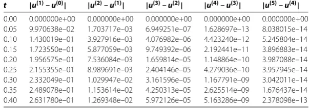
In order to illustrate fast convergence of Newton’s iterations we provide numerical ex-amples with D = ,D= ., D= ., and u, v being sample piecewise polynomial
functions taking values in [., .]. We check the differencesuk+–ukandvk+–vkfor
k= , , , , . Our computer programs are performed by implicit finite difference meth-ods with stepsh=h= .; see Table (direct iterations), Table (Newton’s iterations).
Appendix
Lemma A. Assume that
z(t)≤
t
C
√
t–sz(s)ds+
t
˜
C
(t–s)αp(s)ds and p(s)≤Ks
m.
Then z(t)≤ ˜K tm+αfor t∈[,T],where
Table 1 Maximal differences between successive approximationsu(k)by direct iterations (3.1) withD1= 1,D2= 0.5,D3= 0.2,h= 0.01,h0= 0.01
t |u(1)–u(0)| |u(2)–u(1)| |u(3)–u(2)| |u(4)–u(3)| |u(5)–u(4)|
0.00 0.000000e+00 0.000000e+00 0.000000e+00 0.000000e+00 0.000000e+00 0.05 1.023328e–01 3.742852e–03 1.383520e–04 7.409068e–06 3.256123e–07 0.10 1.476173e–01 6.990620e–03 2.908263e–04 1.835346e–05 1.004908e–06 0.15 1.783626e–01 9.324930e–03 4.031573e–04 2.746097e–05 1.675459e–06 0.20 2.028066e–01 1.096861e–02 4.788241e–04 3.397007e–05 2.215127e–06 0.25 2.239067e–01 1.206830e–02 5.253484e–04 3.806322e–05 2.601687e–06 0.30 2.425240e–01 1.273201e–02 5.499511e–04 4.011546e–05 2.844953e–06 0.35 2.593736e–01 1.304597e–02 5.585483e–04 4.051817e–05 2.967818e–06 0.40 2.745434e–01 1.307759e–02 5.556250e–04 3.970391e–05 2.985870e–06
Table 2 Maximal differences between successive approximationsu(k)by Newton’s method (4.1) withD1= 1,D2= 0.5,D3= 0.2,h= 0.01,h0= 0.01
t |u(1)–u(0)| |u(2)–u(1)| |u(3)–u(2)| |u(4)–u(3)| |u(5)–u(4)|
0.00 0.000000e+00 0.000000e+00 0.000000e+00 0.000000e+00 0.000000e+00 0.05 9.970638e–02 1.703717e–03 6.949251e–07 1.628697e–13 8.038015e–14 0.10 1.430019e–01 3.927916e–03 4.076982e–06 4.423240e–12 5.245804e–14 0.15 1.723550e–01 5.877059e–03 9.749392e–06 2.192441e–11 3.896883e–14 0.20 1.956575e–01 7.536084e–03 1.659814e–05 1.148864e–10 3.987088e–14 0.25 2.155355e–01 8.989691e–03 2.404146e–05 4.279036e–10 3.957945e–14 0.30 2.332049e–01 1.029947e–02 3.161596e–05 1.167791e–09 3.042011e–14 0.35 2.489078e–01 1.153614e–02 4.250313e–05 2.625514e–09 1.676437e–14 0.40 2.631780e–01 1.269348e–02 5.972126e–05 5.163286e–09 2.378098e–13
Proof We have
z(t)≤
t
C
√
t–sz(s)ds+
t
˜
C
(t–s)αKs
mds
≤
t
C
√
t–sK t˜
m+αds+ t
˜
C
(t–s)αKs
mds
for ≤t≤T and≤α< . We claim that
K Ct˜ m+αT/+CKt˜ m+α
θm
( –θ)αdθ≤ ˜K t
m+α,
˜
K tm+α – CT/≥ ˜CKtm+α
θm ( –θ)αdθ.
It suffices to take
˜
K:=K C˜
– CT/
θm
( –θ)αdθ. (A.)
Competing interests
The authors declare that they have no competing interests.
Authors’ contributions
Acknowledgements
This work was supported by the National Science Center (Poland) decision no. DEC-2011/02/A/ST8/00280.
Received: 31 January 2014 Accepted: 9 April 2014 Published:#PUBLICATION_DATE
References
1. Darken, LS: Diffusion, mobility and their interrelation through free energy in binary metallic systems. Trans. AIME174, 184-201 (1948)
2. Kirkendall, EO: Diffusion of Zinc in Alpha Brass. Trans. AIME147, 104-110 (1942)
3. Holly, K, Danielewski, M: Interdiffusion in solids, free boundary problem forr-component one dimensional mixture showing constant concentration. Phys. Rev. B50, 13336-13346 (1994)
4. van Dal, MJH, Gusak, AM, Cserhati, C, Kodentsov, AA, van Loo, FJJ: Microstructural stability of the Kirkendall plane in solid-state diffusion. Phys. Rev. Lett.86, 3352-3355 (2001)
5. Danielewski, M, Wierzba, B: Thermodynamically consistent bi-velocity mass transport phenomenology. Acta Mater.
58, 6717-6727 (2010)
6. Bellman, R: Methods of Nonlinear Analysis. vol. II. Academic Press, New York (1973)
7. Bellman, R, Kalaba, R: Quasilinearization and Nonlinear Boundary Value Problems. Am. Elsevier, New York (1965) 8. Mlak, W, Schechter, E: On the Chaplyghin method for partial differential equations of the first order. Ann. Pol. Math.
22, 1-18 (1969)
9. Koleva, MN, Vulkov, LG: Two-grid quasilinearization approach to ODEs with applications to model problems in physics and mechanics. Comput. Phys. Commun.181(3), 663-670 (2010)
10. Chaplygin, SA: Collected Papers on Mechanics and Mathematics. Moscow (1954) 11. Kantorovich, LV, Akilov, GP: Functional Analysis in Normed Spaces. Pergamon, Oxford (1964)
12. Friedman, A: Partial Differential Equations of Parabolic Type. Prentice Hall International, Englewood Cliffs (1964) 13. Kiguradze, I: On solvability conditions for nonlinear operator equations. Math. Comput. Model.48, 1914-1924 (2008)
#DIGITAL_OBJECT_IDENTIFIER
Cite this article as:Leszczy ´nski and Wrzosek:Iterative methods for ternary diffusions.Boundary Value Problems