Catchment scale modelling of micro and emerging pollutants

Curriculum 1. Civil and En_{vironmental Engineering}

Elena Diamantini

Catchment scale modelling of micro and

emerging pollutants

Mechanical Engineering

- Do cto

Except where otherwise noted, contents on this book are licensed under a Creative Common Attribution - Non Commercial - No Derivatives

4.0 International License

University of Trento

Doctoral School in Civil, Environmental and Mechanical Engineering http://web.unitn.it/en/dricam

Via Mesiano 77, I-38123 Trento

Doctoral Thesis - April 2018

ELENADIAMANTINI

Catchment scale modelling of micro and

emerging pollutants

Supervisor:

T

he fate and transport of solutes introduced into a watershed and sampled at the catchment

outlet depends on many environmental, chemical and hydro-climatological forces. Moreover, if the solutes are micro and emerging pollutants (i.e. pharmaceuticals), which are non-regulated contaminants not routinely monitored but often-detected in fresh waters, the description of the transport sources and routes becomes an interesting and challenging topic to investigate and describe, especially in conjunction with the well-known travel time transport approach at the

catchment-scale. In fact, with the travel time approach to

pharmaceuticals represents a framework that allows dealing in a unitary and simple way the main two mitigation mechanisms controlling them, which are dilution and biological decay. Moreover, possible consequences on the health of humans and of aquatic organisms have become issue of increasing concern by the scientific community worldwide. The topics have been extensively studied in the last decades, with some recent benchmark contributions. Nevertheless, there is still room for further development for emerging contaminant models and there is still the necessity of complementing the applications with measured data. This doctoral thesis aimed at contributing with new insights into the multi-faceted aspects of solute

transport at catchment-scale, proposing novel solutions, with applications to real-world case studies and including a detailed description of the major aspects that influence the water quality dynamics in rivers. The thesis is divided into three

accurate analysis of existing information is therefore useful and necessary to identify stressors that may act in synergy and to design new field campaigns. In addition, a detailed data analysis of the main water quality variables is presented: advanced statistical analyses (i.e. Spearman rank correlation, Principal Component Analysis, and Mann-Kendall trend tests) were applied to long-term time series of water quality data both in the Adige River Basin and in the Ebro and Sava catchments, aiming at providing an integrated and comparative analysis of recent trends, in order to investigate the relationships between water quality parameters and the main factors controlling them (i.e. climate change, streamflow, land use, population) in the

Mediterranean region. These catchments are included into the EU project “Globaqua ”, dealing with the analysis of the

combined effect of several stressors on the freshwater

ecosystems in Mediterranean rivers. In fact, little attention has been paid to linkages between long-term trends in climate, streamflow and water quality in European basins; nevertheless, such analysis can represent, complementary to a deep

knowledge of the investigated systems, a reliable tool for

decision makers in river basin planning by providing a reliable estimate of the impacts on the aquatic ecosystem of the studied basins. In the second part, sampling campaigns performed in our study basin, the Adige catchment, are presented in detail. Special attention is also given to emerging pollutants, whose study on the occurrence patterns and spatiotemporal variability in the Adige River Basin has been conducted in conjunction with population patterns and touristic fluxes. In the third and last part, novel theoretical solutions of the well-known

W

hen I started this PhD, I was not completely consious of the multitude difficulties that I would have encountered on the path. Nevertheless, I did not realise how the PhD could represent a training process both as a researcher and as a woman; only now I can assert that surely it has been a truly life-changing experience for me and it would not have been possible to achieve without the support of many people. Foremost, I would like to express my limitless gratitude to my supervisor, prof. Alberto Bellin for his scientific contribution but, most of all, for his support, guidance and encouragement, in particular during the last period of my PhD path.

I gratefully acknowledge the Department of Civil and

Environmental Engineering at the University of Trento for both the financial support and for helping me disentagle the

bureaucracy.

A very special acknowledgement goes to the people of my reasearch group: Bruno, Diego, Oscar, Alessandra, Giorgia and Gabriele. Thank you for sharing your work, your life experiences and for all the good advices.

During these three amazing years I made a lot of unexpected friends, many of whom were also my office mates and my colleagues: Karina, Simone, Ines, Elisa and Marialaura. I will always remember all the time we had spent toghether and I hope we may meet again some time in the future. Surely I am forgetting someone, so please excuse me.

A heartfelt thank goes to my old but not “dated ”friends: Renato, Martina, Roberta and Alice.

me and encouraging me to follow my dreams; thank you for all your love and support and mostly thanks for all of the sacrifices that you have made on my behalf. As I said you some years ago, long-distances do not constitute an obstacle to help each other and support all our difficulties. Your solace, you ability to

listening and supporting, and your motivation were fundamental in these years.

Page

List of Tables ix

List of Figures xi

1 Introduction 1

1.1 Data analysis of existing water quality variables of

European rivers . . . 4

1.2 Contamination sources and distribution patterns of pharmaceuticals in the Adige River Basin . . . . 6

1.3 Catchment scale transport model of micro and emerging pollutants . . . 8

2 Study basins, data and methods 13 2.1 Study basins . . . 13

2.2 Data . . . 16

2.2.1 Existing water quality variables . . . 16

2.2.2 Experimental sampling campaigns . . . 22

2.2.3 Data for transport model . . . 27

2.3 Methods . . . 30

2.3.1 Statistical analyses . . . 30

3.1.1 Trends in drivers . . . 43 3.1.2 Correlation analysis . . . 46 3.1.3 Mann-Kendall trend test . . . 50 3.2 Contamination sources and distribution patterns

of pharmaceuticals and personal care products in the Adige River Basin . . . 62 3.2.1 Occurrence and spatial distribution of

se-lected PPCPs in winter . . . 62 3.2.2 Occurrence and spatial distribution of

se-lected PPCPs in summer . . . 69 3.3 Transport model of micro and emerging pollutants 80 3.3.1 Inference of the model parameters . . . 80 3.3.2 Application at catchment scale . . . 89

4 Conclusions 97

4.1 Driver detection of existing water quality trends in the Adige, Ebro and Sava catchments . . . 97 4.2 Contamination sources and distribution patterns

of pharmaceuticals and personal care products in the Adige River Basin . . . 99 4.3 Transport model of micro and emerging pollutants 100

TABLE Page

2.1 Water quality variables included in the study, mean values and ranges in the period 1990-2015. . . . 19 2.2 Coefficients for the definition of™and©. . . 34

3.1 Mean discharges for each sampling site and for both sampling campaigns: Q_{f eb} are the average values of hourly water discharges in the period 15/02-18/02, whereas Q_lug are the average values of hourly water discharges in the period03/07-05/07 . . . 63 3.2 List of the pharmaceutically active compounds and the

associated pharmaceutical classes detected in the Adige Basin samples. . . . 64 3.3 Resident population and touristic fluxes reffered to

each sampling site - winter sampling . . . 65 3.4 Resident population and touristic fluxes reffered to

each sampling site - summer sampling . . . 66 3.5 Theoretical load coefficients (∞) and coefficients of

de-cay (∑) for the 5 pharmaceuticals. . . . 86 3.6 List of the 26 WWTPs of the Adige River basin used

FIGURE Page

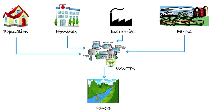
1.1 Main sources of micro and emerging pollutants (i.e., pharmaceuticals and personal care products) in the aquatic ecosystem. . . . 7

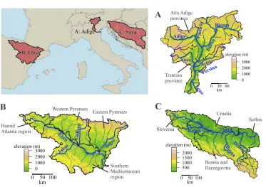
2.1 Map presenting the locations of the study river basins: A) Adige B) Ebro and C) Sava with main regions and tributaries. Digital elevation models (DEMs) are also presented as coloured maps. . . . 14

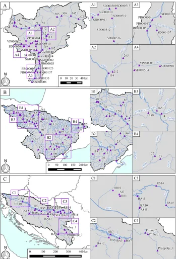
2.2 Locations of water quality sampling stations for Adige (A), Ebro (B) and Sava (C), respectively. Identifiers refer to the original codes as retrieved from the case-specific water agencies. For the station codes see [53]. Right-side picture enlargements show regions with a high station density. . . . 21

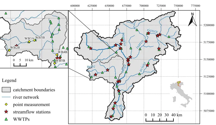
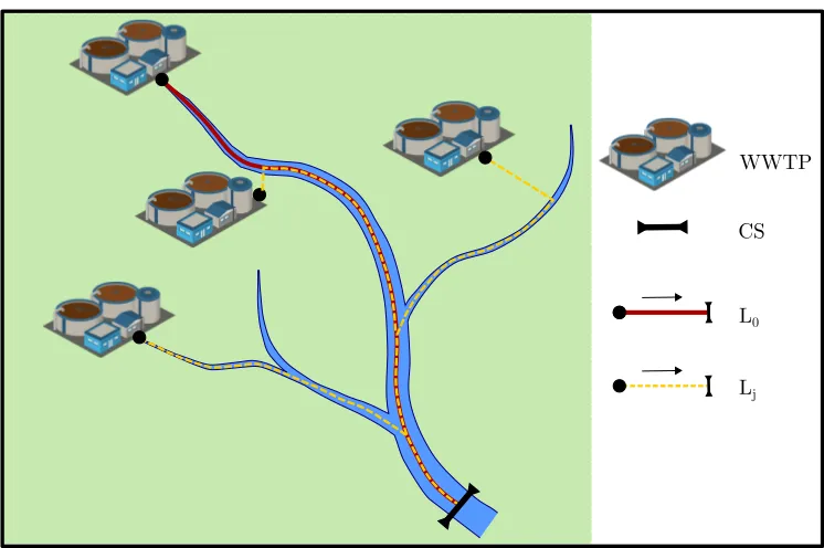
2.4 Map of the Adige River basin and its main tributaries with a zoom of the Noce River basin (upper panel). Green triangles represent the main WWTPs whereas red stars the main streamflow gauging stations. Only for the Noce basin, yellow diamonds symbolize point measurements of the two sampling campaigns (i.e., February and July 2015). . . . 30 2.5 Example of the model scheme: WWTPs that release

con-taminant to both the main stem and its tributaries are considered as point injections of pharmaceuticals. The distance between each WWTP and the river is calcu-lated as the shortest orthogonal line between the two points. The distance between the release and the Con-trol Section (CS) is defined as L0 if the WWTP is

lo-cated in the initial section of the basin whereas L_j if the WWTP belongs to tributaries of the main stem or if it is situated downstream the initial section. . . . 41

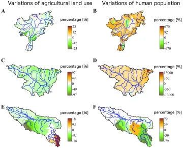
3.1 Sen’s slope trend magnitudes of monthly specific stream-flow (left) and monthly air temperature (right) for Adige (A, B), Ebro (C, D) and Sava (E, F), respectively. Changes for both drivers refer to the period 1990-2015. In order to make the time series of the three basins comparable, streamflow time series were normalised by the drainage area at the sampling point. . . . 44 3.2 Relative changes in the proportion of agricultural land

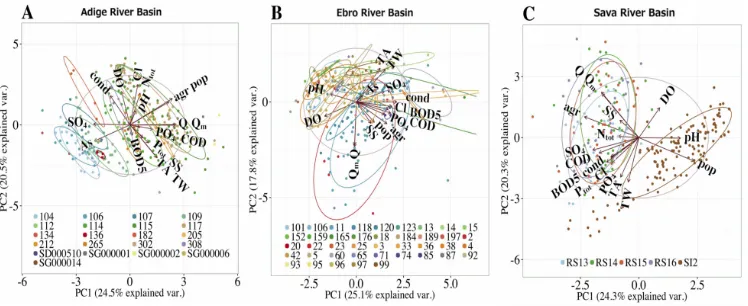
3.3 Matrices of mean Spearman correlation between vari-ables and drivers (black rectangles) for Adige (A), Ebro (B) and Sava (C) river basins obtained by averaging the correlation coefficients identified for each sampling location; red and blue dots correspond to negative and positive correlations, respectively. Small dots with light colour intensity represent low correlations while big dots with darker colours correspond to higher corre-lations. The rows in the correlation matrices referring to the drivers, which are agricultural land use (agr), population (pop), monthly mean water discharge (Qm) and monthly mean temperature (TA), are included in a rectangular box. . . . 47

3.5 MK mean trends (expressed as annual percentages of variation with respect to mean concentrations) on a moving time window of 10 years in the period 1990-2015 for the 6 water quality variables averaged over all the water quality stations of each basin. The abscissa shows the initial time of the 10 years window; there-fore, the trend associated to the year 1990 is computed over the time window 1990-1999, and the trends for the following years up to 2006 are determined accord-ingly. Thick lines represent the mean trend whereas light colours indicate uncertainty bands expressed by standard deviation. . . . 51

3.6 Significant MK trends over the period 1990-2015 for the stations of Adige (A), Ebro (B) and Sava (C) river basins, respectively. Direction of triangles expresses the Sen’s slope trend sign, whereas colours represent the driver with the maximum absolute value of Spearman corre-lation with the water quality parameter. Lines inside each triangle indicate a negative correlation between variables and the respective drivers; the absence of lines indicates positive correlations. . . . 54

3.7 Pie charts with percentages of pharmaceuticals con-centrations detected in surficial waters during winter sampling campaign, associated to the sampling loca-tions within the Adige River Basin. Pharmaceuticals were aggregated by class. . . . 67

3.9 Pie charts with percentages of pharmaceuticals concen-trations detected in sediments during winter sampling campaign. Pharmaceuticals were aggregated by each family. . . . 69

3.10 Concentrations of pharmaceuticals detected in sedi-ments during winter campaign, specified for each sam-pling point. . . . 70

3.11 Pie charts with percentages of pharmaceuticals con-centrations detected in surficial waters during summer sampling campaign. Pharmaceuticals were aggregated by each class. . . . 71

3.12 Total concentrations of PCPs in water samples at all sampling locations: summer period. Notice the loga-rithmic scale of the ordinate. . . . 72

3.13 Pie charts with percentages of pharmaceuticals con-centrations detected in sediments during summer sam-pling campaign. Pharmaceuticals were aggregated by each class. . . . 73

3.14 Concentrations of pharmaceuticals detected in sedi-ments during summer sampling campaign, specified for each site. . . . 73

3.16 Error matrices of the 5 selected pharmaceuticals for both winter and summer campaigns. Each dot repre-sents the value of the objective function (L) for each pair of∞and k selected using the Latin Hypercube

proce-dure. Green dots represent high values of L whereas red dots low L values. The best set of parameters is selected among the minimum of the red dots. . . . 88 3.17 River mean concentrations of (A) diclofenac, (B)

keto-profen (C) clarithromycin (D) irbesartan (E) sulfamethox-azole in the Adige catchment relatively to the year 2015. Points and the relative progressive numbers are associ-ated to each WWTP included in the simulation. For the progressive numbers see Table 3.6. Blue colors represent low simulated mean concentrations (range of0_°100 ng/L) whereas red ones represent high simulated mean concentrations (range of1,000_°2,500ng/L). . . . 92 3.18 Concentrations patterns of the 5 selected

pharmaceu-ticals in 10 illustrative streamflow gauging stations within the Adige River Basin in the 2015. Different col-ors represent different pharmaceuticals. . . . 95

C

HA

P

T

1

I

NTRODUCTION

The anthropogenic pressure on water resources is growing worldwide, and reducing its effects on the ecosystem is one of the major challenges to target in the near future

[20, 100, 115, 136, 188]. Acquaintance of the complex ties between hydrological, geochemical and ecological stressors in large river basins (e.g., 10,000 km2or more) is still erratic and further researches are needed to support decisions about water resources management at the catchment scale [12, 36, 158, 191]. Even more complex but appropriate operational strategies may be prioritized,considering economical and societal constraints [25, 183].

on freshwater ecosystems is also an open issue for large catchments. In particular, the inclusion of feedback

mechanisms, which associate ecosystem functioning and anthropogenic activities to water resources management and chemical fluxes [81], represents a challenge. In order to examine these three topics, i.e., changes in the hydrological traits of large catchments, the fate and transport of pollutants in the

environment and the interaction with the ecosystem (including human activities), it is crucial to have access to all available information. In particular, it is necessary, for gaining a global perspective, to integrate data collected by water authorities and environmental protection agencies operating in the river basin, whose results are published in both peer reviewed journals as well as in technical reports and other types of gray-literature (e.g.[182]). Nevertheless, a data integration of other chemicals not routinely monitored but detected in surficial waters must be planned and perfomed.

The present thesis is structured as follows:

° Chapter 2 presents a description of the study basins (2.1), of the available data (2.2), including the information gathered through ad-hoc sampling campaigns, and introduces the statistical methods adopted for the analyses and the

mathematical framework of a novel transport model (2.3);

° Chapter 3 shows the main outcomes of the driver detection of water quality trends in three large European river basins (3.1), a survey on the contamination sources and

distribution patterns of pharmaceuticals and personal care products in a large Alpine river basin (3.2) and the

° Chapter 4 finally draw the conclusions of the main research topics presented in the previous chapters.

In detail, in the first part of this thesis, we provided a review of the "state-of-art" of water quality in surficial waters of three large European river basins among the six included in the GLOBAQUA project [136]. The selection of these basins was realised according to differences in hydro-climatic conditions and land use management, and to their contrasting resilience to climate change. The description of the studied basins is

presented in Sec. 2.1. Particular attention was drawn to the Adige River, selected as study site for most of our analyses. An accurate decription of the three watersheds and their main stressors was presented, beliving that a detailed analysis of existing information is useful and necessary to identify the main stressors that may play in synergy. Moreover, we explored the complex interaction between water quality trends and the main stressors (from now on also called as drivers) observable at large scales and influencing the quality of surficial waters, by

analysing whether observed changes are consistent with their drivers. From this part, we published a review article [39] and two papers [53, 116] in a top journal in the field of science and engineering .

occurrence patterns of contaminants in relation to their sources (tourist arrivals, resident population), and at relating the

temporal variability (summer-winter) of pharmaceuticals and personal care products (PPCPs) to the varying environmental variables (water flow, temperature), in water and sediments. From this part, we published two papers [102, 119].

Finally, in the third and last part of the thesis we defined a new parsimonious, in term of parameters, in-stream transport model which includes and counterbalances the simultaneous effects of dilution, dispersion and decay of pharmaceuticals in surface waters. As a validation, the model is applied to the main

pharmacological classes of our main study cacthment, the Adige River Basin. Two manuscripts describing these methodology and with some applications are in preparation.

1.1 Data analysis of existing water quality

variables of European rivers

The ecological and chemical status of freshwater has attracted significant attention in the last decades (e.g.,[4, 185]). Water bodies hosting important ecosystems are subject to

anthropogenic and climatic stressors often acting in synergy. In order to estimate the effects of these actions aiming at

improving the ecological status of freshwater ecosystems,

monitoring networks have been implemented in the majority of European basins, providing a quite extensive database of water quality parameters [21]. Despite this wealth of data, the

connection between the main drivers and water quality

capability of understanding ecosystem responses to multiple stressors [64], and as a consequence, the possibility for water and land use managers to determine suitable adaptive strategies for mitigating their effects. Many studies described observed changes in chemical, ecological or hydrological variables (e.g., [27]), but few studies attempt to attribute causes of pattern variations [112]. Other works attempted to explain

concentration patterns by using measurements of single experimental sampling campaigns without considering long temporal variations (e.g.,[102]). Moreover, few studies evaluated long-term trends in water quality indicators at single gauging stations or detect alterations in the spatial patterns, chiefly because of data fragmentation and sampling discontinuity [108, 189]. In this first part of the present thesis, we explores the complex interplay between water quality trends and the main drivers discernible at large scales and affecting surface water quality, by analysing whether observed changes are consistent with the drivers of change. To this aim, three large European river basins among the six included in the GLOBAQUA project [136] are studied: Adige, Ebro and Sava. The selection of these basins is made according to differences in hydro-climatic conditions and land use management, and to their contrasting resilience to climate change [116]. The main objectives of the first part are:

(i) analysing long term water quality trends in each selected river basin;

(i i) identifying links between observed patterns of

(i i i) comparing the studied basins with respect to their vulnerability and resilience to the identified drivers of change.

1.2 Contamination sources and distribution

patterns of pharmaceuticals in the Adige

River Basin

Beyond the analysis of the classical measured physico-chemical water parameters in rivers, it is worth including and analysing also solute emerging pollutants, whose concentrations in the environment are of increasing concern. With this term, we include synthetic or naturally occurring chemicals, not

commonly monitored in the environment but which have the potential to enter the acquatic environment and cause known or suspected adverse ecological and human health effects. The term "emerging" is also used to describe not the pollutant itself, but rather a new "emerging concern", i.e., newly demonstrated toxic effect and/or mechanism of action of an old pollutant [19]. They are categorised into more than 20 classes related to their origin. The prominent classes are: pharmaceuticals, personal care products (PPCPs) (i.e., prescription drugs, non-prescription drugs, veterinary drugs and consumer chemicals typically found in fragrances, sun-screen agents, lipsticks, shampoos, hair colors and cosmetic products [28, 49]), pesticides, disinfection

by-products wood preservation and industrial chemicals. In particular, PPCPs are considered emerging contaminants and can enter the aquatic ecosystem through multiple pathways, including human excretion, unused drugs and products, agricultural and livestock practices [28, 95, 141, 160, 179].

wastewater treatment [71, 87, 176]. Because of this continuous release into the aquatic environment, PPCPs may act as

pseudo-persistent contaminants [59], and as such may cause undesired and unexpected effects on the living organisms and environment [50, 61, 63, 174].

Figure 1.1:Main sources of micro and emerging pollutants (i.e.,

phar-maceuticals and personal care products) in the aquatic ecosystem.

PPCPs in the aquatic environment have been recognized as one of the most urgent environmental issues during the last decade [94]. Concentrations of PPCPs range fromng L°1toµg L°1, while

their occurrence in water varies across different regions and seasons [98, 130, 173]. Moreover, the relevance of PPCPs

associated with touristic activity in Alpine ecosystems is largely unknown. So far, the impact of tourism on river water quality has mostly been approached through the monitoring of the physicochemical and microbiological parameters [9, 23]. Even though several studies have reported concentrations of PPCPs in large rivers [127], papers regarding the occurrence of PPCPs in the Alpine streams are limited in number (see e.g., [151].

Alpine regions requires further investigation. In this context, our experimental catchment, the Adige River Basin, may be

considered a representative basin with intense touristic activity both in summer and winter months. As a consequence, strong seasonality on consumption and use of PPCPs and their drain to the river system is likely to be expected. Waste water treated effluents have been identified as the main sources of

contamination in the Adige catchment, while extensive

hydropower exploitation [194], which has induced significant alterations of the streamflow regimes in both the main stem and tributaries [117] is likely to enhance the sensitivity of the river ecosystem to PPCP loads. Therefore, the present study aims at:

(i) defining the occurrence patterns of contaminants in relation to their sources (tourist arrivals, resident population);

(i i) relating the temporal variability (summer-winter) of PPCPs to the varying environmental variables (water flow,

temperature), in water and sediments.

The mathematical framework at the basis of this analysis is described in Sec. 2.3.1, while the results are presented in Sec. 3.2.

1.3 Catchment scale transport model of micro

and emerging pollutants

The presence of pharmaceuticals in the environment has posed a wealth of attention in the last decades, as these non regulated emerging contaminants are not frequently monitored but often detected in fresh waters in the range of nanograms to

micrograms per litre [2, 59, 104, 152]. It is a common knowledge that the main route of entry of pharmaceuticals as well as

removal efficiency is dependent on the treatment processes and technology [75, 145, 156]. Owing to the concurrent effects of the increase in the use of drugs, often due to an increase in

population and an improvement of health conditions, and the low pharmaceuticals removal efficiency of wastewater treatment plants, ubiquitous concentrations of pharmaceuticals in fresh waters have been detected. Possible consequences on the health of humans and of aquatic organisms have become issues of increasing concern by the scientific community worldwide [28, 85, 165]: disruption of human endocrine functions,

developmental defects in fish and other organism, alterations in the survival, growth, and reproduction of a species, and the promotion of antibiotic resistance are just few examples

[30, 40, 83]. For those reasons, the European Union, through the Directive 2013/139/EU, attempted to prevent the diffusion of pharmaceuticals in the aquatic environment by defining environmental quality standards and by pinpointing priority substances that could represent a potential risk. Furthermore, attempts to evaluate predicted concentrations in fresh waters have been made through many emerging contaminant models, among which the two most widely applied GIS-based models are PhATE (Pharmaceutical Assessment and Transport Evaluation [11]) and GREAT-ER (Geography-Referenced Regional Exposure Assessment Tool for European Rivers [60]). In order to be applied and corroborated, the two models need a huge amount of data in field conditions often difficult to obtain in field studies or in non-instrumented large basins [77]. It is well known that when modeling emerging contaminants the available information is limited and, therefore, simpler models are usually more useful than complex ones [7]. Nevertheless, more refined and higher tiered models will presumably result in more accurate

data and more computing time [60]. Moreover, spatial

consumption variation through population, due to differences between resident population and transient (i.e., tourist fluxes) is still missing [8]. In fact, very few studies have analyzed temporal and seasonal variations [47, 114, 157] in both predicted

concentrations and in the estimation of the decay constant, both linked with touristic fluxes. The study of the fate and

transport of pharmaceuticals in rivers, especially in catchments subject to significant touristic fluxes, which may induce

fluctuations in the contaminant load, is in its infancy [43]. For those reasons, there is still potential for further development of emerging contaminant models and there is still the necessity of complementing the applications with measured data [7].

Within this framework, the core of the present thesis aims at

(i) defining a new parsimonious, in term of parameters, in-stream transport model which includes and counterbalances the concurrent effects of dilution,

dispersion and decay of pharmaceuticals in surface waters.

(i i) applying the proposed transport model to the main pharmacological classes in a large Alpine river basin.

Its strength is that the only source needed to model

pharmaceuticals is represented by human resident population and touristic fluxes when present, the latter varying seasonally, both considered as a proxy of the sewage effluents. Human population and touristic fluxes data are easily available and this let the model be applied to every catchments even large and non-instrumented, overcoming the lack of data. Moreover, the model can be easily coupled with existing hydro-climatological models to predict streamflow and water temperatures in

C

HA

P

T

2

S

TUDY BASINS

,

DATA AND METHODS

2.1 Study basins

The Adige River Basin The Adige river rises from a spring in proximity of the Resia lake at the elevation of 1,586 m a.s.l. and after 409 km it ends in the Adriatic sea at Porto Fossone between Brenta estuary and Po river delta. With a contributing area of 12,100 km2, the Adige is the third largest Italian river (after Po and Tiber) and the second longest (after Po). The mean water discharge registered at Boara Pisani gauging station (in the proximity of Rovigo municipality, near the catchment outlet) is about 202 m3/s [52], with peaks usually registered in the period from June to September [146], showing the typical behavior of Alpine catchments.

Figure 2.1:Map presenting the locations of the study river basins: A) Adige B) Ebro and C) Sava with main regions and tributaries. Digital elevation models (DEMs) are also presented as coloured maps.

valley that holds its name. The Adige receives the contribution of the Isarco river, close to Bolzano, and the contributions of both the Noce and Avisio rivers just upstream of Trento, where the drainage area of the Adige river rises, thanks to these

contributions, to 9,810 km2. Finally, it crosses the Lagarina valley until Verona (drainage area of 11,100 km2) and then it turns east again and flows through the Padana plain without receiving other significant contributions. Because of the lack of significant contributions in the lower reach, hydrological studies have been conducted chiefly in the northern part of the

catchment (i.e., Province of Trento and Province of Bolzano). The river basin is divided into 7 main subbasins: Passirio, Isarco-Talvera, Rienza, Noce, Avisio, Fersina, Leno (see Figure 2.1A). In particular, the Noce River is one of the main tributary of the Adige main stem. With a length of 82 km and a total

Ortles-Cevedale and Adamello Presanella groups and flows first to East, but in its middle course it turns to South-East and enters the river Adige close to the municipality of Mezzolombardo a few kilometers North of the city of Trento [117]. The Adige river basin contains 550 lakes, most of which have a surface smaller than 1 ha and of glacial origin [15]. The biggest natural lake is Caldaro, followed by Anterselva, Braies and Carezza in the Province of Bolzano, Lake Tovel and Terlago in the Province of Trento.

The Ebro River Basin The Ebro River Basin is mainly located in the north-eastern part of Spain (Figure 2.1B). With a catchment area of 85,362 km2, the Ebro is the largest river basin of Spain. The basin extends from the Pyrenees and the Cantabrian Range in the north (maximum altitude of more than 3,000 m a.s.l.) to the Iberian Range in the South and the Coastal Range in the East [112]. The Ebro River has a length of 910 km and it drains into the Mediterranean Sea with a mean streamflow of 425 m3/s. Segre, Cinca, Aragón, Gallego, Jalon and Zadorra are the main tributaries of the Ebro River. Long-term mean annual air temperature is 11.4±C and mean annual precipitation is 620 mm (both evaluated in the time span 1920_°2000; [161]. The climate is mostly continental-Mediterranean, since it ranges from semi-arid in the centre of the river valley to oceanic in the Pyrenees and Iberian Mountains.

and Herzegovina (40%), Serbia (15.4%), Montenegro (7.5%), and a minor portion in Albania (0.1%). It is 945 km long and it drains into the Danube in Belgrade (Serbia). Climatic conditions along the river course range from alpine to continental. Long term annual mean temperatures, evaluated between 1971 and 2000, range from 6±C in the mountain regions to 13±C close to the river mouth [139]. Mean annual precipitation, evaluated

between 1961 and 1990, ranges from 800 mm to 1,600 mm [140].

2.2 Data

As anticipated in the introductory chapter, in the first part of the present thesis, we performed a complete data analysis of both surficial water quality variables obtained mainly from the Environmental protection agencies and existing

hydro-climatological data, by using advanced statistical tools. To this aim, we compared the three European river basins

presented in Sec. 2.1. Data used for these first parts are described in Sec. 2.2.1. For the second part of the thesis, the description of the experimental activities performed in the Adige catchement is provided in Sec. 2.2.2, whereas data used in the last parts of the thesis, for the application of the transport model to the Adige catchment, are presented in Sec. 2.2.3.

2.2.1 Existing water quality variables

For reasons of comparability between the three basins, the study period was set from 1990 to 2015: restriction to the time frame was necessary because of the limited availability of

during the study period) were considered in all the three basins to perform trend analyses. Data were organised into two groups: variables and drivers. The former included water quality data used to detect the trends, while the latter included selected important factors available continuously in time at the European scale, i.e., instantaneous and monthly aggregated streamflow, monthly aggregated air temperature, population density and percentage of agricultural land use. The percentage of artificial areas such as "urban fabric", "industrial, commercial and transport units", "mine, dump and construction sites" and "artificial, non-agricultural vegetated areas" (cf. Corine Land Cover class information), was discarded from the analysis due to the similarity in the spatial patterns with population density. Hence, the driver population density was assumed as an indicator of the overall anthropogenic impact. Other determining features were not included in the statistical analyses because of the difficulty to obtain them at monthly time scale and for all the investigated catchments. These include treated and untreated waters, livestock density, industrial

outflows, mining activities, crop choices, and intensity of agricultural production, which may be considered in future studies at smaller scales (e.g., specific regions of large river basins). Nevertheless, annual data of livestock and phosphate fertilisers for the three basins were used in order to support the discussion. Data were downloaded from the Italian institute of statistics (ISTAT,ht t p :

//ag r i.i st at.i t/sag_i s_pd wout/j sp/Intr oduzi one.j sp, 2016) for the Adige basin and from the Food and Agriculture Organization of the United Nations (FAOSTAT,

2003_°2015 and 2002_°2016, respectively, but aggregated at regional scale, which is wider than the Adige catchment of about 3,000 km2. For the Ebro, the data refer to the whole area of Spain. Phosphate fertiliser data are available for the period 2002_°2014 and livestock data for the period 1990_°2014. Finally, for the Sava, data are aggregated at each national scale (i.e., Croatia, Serbia, Montenegro, Slovenia, and Bosnia and Herzegovina) over periods that vary depending on the country. For phosphate fertilisers, the longest period is 2002_°2014, while for livestock density, the longest period is 1992_°2011 only for Bosnia and Herzegovina, Croatia and Slovenia.

Physico-chemical variables were available at monthly resolution at 45, 42 and 22 monitoring stations in the Adige (Figure 2.2A; http://www.appa.provincia.tn.it;

http://www.provincia.bz.it/agenzia ambiente/), Ebro (Figure 2.2B; http://www.datossuperficiales.chebro.es:81/WCASF/) and Sava (Figure 2.2C; http://www.icpdr.org/wq-db/), respectively. The dataset used in this work includes only variables, selected from larger sets of parameters, that are in common among the three basins: pH, water temperature (TW), electrical

conductivity (cond) and concentrations of arsenic (As),

biological oxygen demand (BOD5), chemical oxygen demand (COD), dissolved oxygen (DO), total nitrogen (Ntot), phosphates (PO4), total phosphorus (Ptot), chloride (Cl), suspended solids (SS) and sulphates (SO4). All variables are expressed in mg L°1 except pH [_°], electrical conductivity [µScm°1] and water and

Table 2.1:Water quality variables included in the study, mean values and ranges in the period 1990-2015.

Instantaneous streamflow time series (Q) were retrieved from the hydrological offices of the Provinces of Trento

(ht t p: //w w w.f lood s.i t/publi c/i ndex.php) and Bolzano (ht t p: //w w w.pr ovi nci a.bz.i t/hydr o/i ndex_i.asp) for the Adige, and the Confederación Hidrográfica del Ebro (CHE) for the Ebro. For the Sava, daily streamflow were obtained from the Global Runoff Data Centre portal (GRDC,ht t p:

//w w w.ba f g.de/GRDC/E N/Home/homepag e_node.html), the TransNational Monitoring Network (TNMN

ht t p: //w w w.i cpdr.or g/w q_°db/) and national water agencies of the countries crossed by the Sava (Environmental Agency of the Republic of Slovenia, ARSO,w w w.ar so.g ov.si; Hrvatske vode,w w w.vod a.hr; and Republic

Hydrometeorological Service of Serbia,w w w.hi dmet.g ov.r s). When streamflow is not available at the water quality monitoring station, it is inherited from the closest gauging station, after rescaling with the contributing area. However, if streamflow measurements are not available at all the available gauging stations in the same period of water quality sampling, or the closest gauging station is too far away, the respective

concentrations are discarded prior to analysis [116]. Coupled with Q time series, monthly aggregated data (Q_m) were also introduced as a proxy of the seasonality of the hydrological cycle. Monthly time series of air temperature (TA) were extracted from the version 12.0 of the 0.25 [±C] resolution E-OBS gridded

a more detailed small-scale analysis of industrial activities, including mine production and agriculture, may provide additional insights, available data currently do not allow this type of analysis. Population data at an interval of 5 years from 1990 to 2015 were obtained from NASA

Socioeconomic-Data-and-Applications-Center (downloaded from

http://beta.sedac.ciesin.columbia.edu/data/collection/gpw-v4/sets/ browse, 2017). For each river basin, drainage areas at the sample locations were determined from the European-wide digital elevation model provided by the GMES RDA project (downloaded from

http://www.eea.europa.eu/data-and-maps/data/eu-dem, 2017). Annual population and agriculture data were then aggregated at the level of the single sub-basin by linearly interpolating

between the two closest years with information in the dataset.

2.2.2 Experimental sampling campaigns

Pharmaceuticals and personal care products (PPCPs)

concentrations in the Adige River Basin were obtained during two extensive sampling campaigns performed in 2015 (February 15th - 18th and July 3r d - 5th, 2015) in twelve selected sites (see Figure 2.3). The list with the code, name and reasons of the selection is the following:

• WB1 (i.e.: 1): Bresimo in the Noce catchment. Reference site in almost pristine conditions;

• WB2A and WB2B (i.e.: 2A and 2B): downstream WWTP of the Tonale pass in the Noce catchment. Example of

• WB3A and WB3B (i.e.: 3A and 3B): downstream WWTP of Mezzana in the Noce catchment. Example of headwater impacted by both WWTP release and hydropeaking;

• WB4B (i.e.: 4B): downstream S. Giustina reservoir in the Noce catchment. Lower course of the Noce at

Mezzocorona, downstream of two reservoirs in series, one with large capacity;

• WB5B (i.e.: 5B): downstream Mezzocorona power plant in the Noce catchment. Lower course of the Noce at

Zambana, downstream WB4B and the restitution of a large hydropower plant;

• WB6B (i.e.: 6B): located in the main stem of the Adige at Faedo upstream the city of Trento and the main tributaries in the Trentino region (Noce, Avisio and Fersina);

• WB7A, WB7B, WB7C and WB7D (i.e.: 7A, 7B, 7C, 7D): four sites between Mattarello and Rovereto, downstream the city of Trento, in the Adige main stem. Example of

headwater impacted by human activities.

For the sake of simplicity, the prefix "WB" (i.e. Water Body) in Figure 2.3 was omitted.

Sediment samples were collected with a small inox spade from the uppermost 10 cm sediment layer of both left and right banks and then mixed. Hence, they were sieved on site with a 2 mm mesh sieve. Samples were subsequently stored in high-density polyethylene (HDPE)_Æ88 1 L bottles. Liquid samples, taken on the top of the water level, were collected on the left, center and right river side and then mixed. Water samples for the analysis of pharmaceutically active compounds (PhACs) were stored in 1 L gray PE bottles, while water samples for the personal care

bottles. Afterwards, samples were transported to the laboratory in a refrigerated isothermal container (dry ice) and stored at°20 ±_{C until extraction. Water temperature and specific electrical}

conductivity at the standard temperature of 25±C were

measured with an Aquatroll 200 multi-parameter probe, while turbidity was measured by a Ponsel IR optical turbidimeter. River velocity was measured by a Decatur Electronics Europe Inc. radar gun 2016. Regarding sample preparations and analysis, all chemical standards used in this research were of high purity grade (_>90%). Following the preparation,

standardswere stored on_°20±C. Fresh stock antibiotic solutions were prepared every month due to their limited stability while the stock solutions for the rest of substances were renewed every three months. In particular, regarding the pharmaceutically active compounds (i.e., PhACs), the analysis in water samples was conducted following the method developed by [74]. The analyses were carried out with an off-line solid phase extraction (SPE) followed by ultrahigh- performance liquid

chromatography coupled to triple quadrupole linear ion trap tandem mass spectrometry (UHPLC-QqLIT-MS2).

Chromatographic separations were carried out with a Waters Acquity Ultra-PerformanceT M liquid chromatography system, coupled to a 5,500 QTRAP hybrid triple quadrupole-linear ion trap mass spectrometer (Applied Biosystems, Foster City, CA, USA) with a turbo Ion Spray source. Moreover, the target

analytes were eluted from the column into the chromatograph with the LC-mobile phase, and the separation was achieved with two binary pump systems (Milford, MA, USA), using an Acquity HSS T3 column (50 mm x 2.1 mm i.d., 1.8µmparticle size) for

electrospray ionization (NI), both purchased fromWaters Corporation. Electrospray Ionization (ESI) and the reaction monitoring (SRM) modes were selected for the MS2 detection. Prior to the instrument analysis, standard mixture containing all isotopically labeled standards was added in the extracts as an internal standard. Quantification was carried out by isotope dilution. The analysis of PhACs in sediment samples was carried out according to the method developed by [93]. Previously freeze-dried and homogenized sediment samples were extracted by pressurized liquid extraction (PLE) using an ASE 300

Accelerated Solvent Extractor (Dionex, Sunnyvale, CA, USA) equipped with 11 mL stainless extraction cells. The extracts of sediment obtained by PLE (_ª22mL) were diluted in 500 mL of HPLC water (methanol_<5%) and processed by SPE using the Oasis HLB cartridges (200 mg, 6 mL). The resulting extracts were evaporated under a gentle stream of nitrogen and reconstituted with the internal standard solution to a final volume of 1 mL. The analyses of the samples were carried out by UHPLC-MS2 in the same analytical platform as for the water samples. The analysis of PCPs in water samples was conducted following the method developed by [67]. The analyses were carried out by on-line solid phase extraction-high performance liquid

chromatography-tandem mass spectrometry (SPE-HPLC-MS2). The analyses were carried out on a Transcend LX System

5µmparticle size) analytical column from Merck preceded by a

guard column LiChroCART 4-4 Purospher STAR RP-18 ec (5µm particle size). Atmospheric Pressure Photo- Ionization (APPI) and SRM modes were selected for the MS2 detection. Before the instrument analysis, a standard mixture containing all

isotopically labeled standards was added in the extracts as an internal standard. Quantification was carried out by isotope dilution. PCPs in sediment samples were determined according to the method by [66], using frozen-dried and homogenized samples. After the addition of the surrogate standards to the samples, the target analytes were extracted by PLE in an ASE-350 Accelerated Solvent Extractor (Thermo Fisher Scientifics). The resulting extracts were brought to 25 mL with MeOH and

aliquots of 2 mL were then filtered using a 0.45µmnylon syringe

filter into LC-vials. These solutions were allowed to evaporate under a gentle stream of nitrogen and reconstituted with the internal standard solution to a final volume of 1 mL. The analyses of the samples were carried out by HPLC-MS2 in the same analytical platform as for the water samples, disabling the on-line configuration. Other experimental conditions were the same as those for water analysis.

2.2.3 Data for transport model

Pharmaceuticals concentrations in the Noce sub-basin were obtained during the same two extensive sampling campaigns performed in 2015 described in the previous section. We

the following (see Figures 2.3 - 2.4, [119]): WB2B - downstream WWTP of the Tonale pass, WB3A and WB3B - downstream the WWTP of Mezzana, WB4B - downstream S. Giustina reservoir and WB5B - downstream Mezzocorona power plant Among the measured pharmaceuticals, a subset of only 5 compounds was selected for the application of the transport model with the criteria of the highest concentrations in both the sampling campaigns. The only exception is Diclofenac, which was

detected only in Febraury sample but it was included because it belongs to the "watch list" of 2013/39/EU. The 5

pharmaceuticals are the following

(https://pubchem.ncbi.nlm.nih.gov/compound):

• Diclofenac: non-steroidal anti-inflammatory drug with antipyretic and analgesic actions;

• Ketoprofen: non-steroidal anti-inflammatory drug, analgesic and antipyretic;

• Clarithromycin: semisynthetic macrolide antibiotic;

• Sulfamethoxazole: sulfonamide bacteriostatic antibiotic. Its broad spectrum of activity has been limited by the development of resistance;

• Irbersartan: nonpeptide angiotensin II antagonist with antihypertensive activity.

Regarding the first-attempt values of the two parameters in the model considered for calibration, the theoretical load coefficient (∞i) was estimated through the available data from WHO

Collaborating Centre for Drug Statistics Methodology (World Health Organization; http://www.whocc.no/) and AIFA (Agenzia Italiana

First-attempt estimation of the coefficient of decay (k_i) were performed through previous available studies.

Location of WWTPs were obtained from Agenzia per la Depurazione of the Province of Trento (https://

adep.provincia.tn.it/Agenzia-per-la-Depurazione-ADEP) and from Province of Bolzano (http: // www.provincia.bz.it/agenzia-ambiente/acqua/cartine-schede.asp for Alto Adige Province). The distances between each WWTP and the measuring points were defined through QGIS, an open source Geographic

Information System (http://www.qgis.org/it/site/).

Resident population and tourist presences were obtained from the census offices of Trento http://www.istat.it/it/ and

https://astat.provincia.bz.it and Bolzano, for the territories of the two provinces. Resident population is considered constant for each year while tourist presences are subject to monthly fluctuation. Both were assigned to each WWTP: according to the municipality served, population data were therefore aggregated. Daily streamflow time series (Q) were retrieved from the

hydrological offices of the Provinces of Trento

(ht t p: //w w w.f lood s.i t/publi c/i ndex.php) and Bolzano (ht t p: //w w w.pr ovi nci a.bz.i t/hydr o/i ndex_i.asp). For the application at the catchment scale, monthly time series were obtained through aggregation of daily streamflow values.

Water temperatures (WT) were provided by the Environmental Protection Agencies of the provinces of Trento

(http://www.appa.provincia.tn.it) and Bolzano

Figure 2.4:Map of the Adige River basin and its main tributaries with a zoom of the Noce River basin (upper panel). Green triangles represent the main WWTPs whereas red stars the main streamflow gauging stations. Only for the Noce basin, yellow diamonds symbolize point measurements of the two sampling campaigns (i.e., February and July 2015).

2.3 Methods

2.3.1 Statistical analyses

R coefficients were calculated in order to identify correlations as general descriptors of the interplay between water quality parameters and drivers. Principal Component Analysis (PCA) is a powerful technique of multivariate data analysis useful for identifying patterns in data [167, 190]. In the present work, PCA was applied separately to the complete dataset (both variables and drivers) of each study basin in order to screen temporal and spatial patterns and to select meaningful synthesis variables facilitating the ensuing analyses. PCA was also used to validate the results of Spearman rank correlation, with the further advantage of encompassing spatial information. Since water quality data follow skewed distributions, trend analyses were performed with the nonparametric Mann-Kendall (MK) test in all river basins [99, 120]. The MK-test does not require a priori assumptions of the underlying distributions and should be preferred to parametric trend tests in the analysis of multiple datasets [88]. In order to calculate the sign and magnitude of trends, Sen’s slope estimator was determined from the

MK-statistics because it does not require the underlying

probability distribution to be Gaussian and it is less sensitive to outliers than the Ordinary Least Square [166]. The statistical significance of trends is defined using a significance level of

Æ=0.1 for Kendall’s p-value. MK trends and Sen’s slope estimator were computed for time series of water quality variables with at least 24 measurements. All statistical and graphical analyses were performed using R statistical software packages (ht t ps: //w w w.r_°pr o j ect.or g).

Regarding the statistical analyses performed in the second part of the thesis, preliminary data analyses to explore the

compounds in each family for each sampling location to

perform pairwise correlation with the tourist arrivals (February and July 2015), and the resident population in each municipality. Pairwise correlations were performed for water and sediment samples. For each calculated probability (p), the significance threshold was set at 0.05.

2.3.2 Transport model: mathematical framework

In the following, we present the mathematical framework developed for the definition of a novel transport model for pollutants in surficial waters. Firstly, we introduce the general catchment scale transient model, and then we applied the steady state version to model pharmaceuticals in the Adige River Basin. The steady state model inherits the same mathematical framework of the transient one but introducing some

assumptions and semplifications.

General transient model Let us consider a parcel of water traveling from its entry point in the hydrological system, the source, and a compliance plane, containing the position where it is detected. The parcel contains an initial mass¢m0 of a reactive solute which is transported within the hydrological system and may undergo chemical transformation. Under this hypothesis, transport can be modeled by the following governing equation:

@Cr

@t =

@ @ª

∑

ÆLv(ª,t)@Cr

@ª °v(ª,t)Cr

∏

+R(ª,t) (2.1)

whereCr [M/L3] is the solute concentration,ª[L] is the

Reactive Advection Dispersion Equation (RADE) written in an orthogonal coordinate system moving with the solute’s particle (see e.g. [17]), where we neglected diffusive flux transverse to the trajectory line [123].

We assume now that the velocity can be approximated as follows:

v(ª,t)=v₀(ª)¡(t) (2.2)

wherev₀is the velocity in a reference stationary state and¡

describes the non-stationary effect introduced by the boundary conditions. A similar hypothesis was introduced in the work by [170]. This class of velocity fields has the property that the trajectory of the particle does not change in time, since it is dictated byv0, while the change in the velocity caused by changes of boundary conditions propagates instantaneously along the entire trajectory. This type of velocity field, is

mathematically convenient and it is consistent with the Instantaneous Unit Hydrograph theory based on the width function, which assumes that flow moves along a fixed drainage network dictated by topography [121]. Nevertheless,

steady-state approximation does not entail that the transport velocity can be spatially constant. In order to implement this refinement, we also introduce the assumption that the velocity varies spatially according to the following power law expression proposed by [107]:

vp =©(A)Q™p(A) (2.3)

expressing thep_°th quantile of the velocityvp [m s°1], as a function of the same quantile of water dischargeQ_p [m3s°1]. In Equation (2.3), A [km2] is the contributing area and©and™are

quantile. The expressions of©and™provided by [54], by using

a dataset of 85 gauging stations in Kansas and Oklahoma, were calculated by the following expression:

©(A)=exp£_°°ÆCA+ØCAln(A)

¢

+°ÆQ+ØQln(A)¢™CA

§

(2.4)

with

™CA(A)=

∑_∞

CA+±CAln(A)

∞Q+±Qln(A) ∏1/2

(2.5)

and finally the exponent™is given by:

™(A)₌1_°™CA(A) (2.6)

In all these expressions A[km2] is the contributing area and the other coefficients are reproduced in the table 2.2 (see also Table 3 of the paper by [54]).

Table 2.2: Coefficients for the definition of™and©.

Hydraulic geometry Æ Ø ∞ ±

factors

CA °3.1802 0.6124 0.8404 0.1130

Q °5.5428 0.7992 2.6134 0.0012

The expression (2.3) is a generalization of the power law

expressionv/Qm introduced in the pioneering work of [107], who noticed that the exponentmvaries in dependence of the contributing area. Under the commonly accepted

approximation that at the network scale the contributing area increases stepwise at the nodes of the network, we assume the velocity spatially uniform within the channels. However,

By substituting the expression (2.2) into Equation (2.1) we obtain:

@Cr

@t =¡(t)

@ @ª

∑

ÆLv0(ª)@Cr

@ª °v0(ª)Cr

∏

+R(ª,t) (2.7)

We limit here to the biogeochemical reaction which can be represented as an irreversible first order decay of the type

R(ª,t)=°kC_r(ª,t), where the first order decay rate may be both

positive, in case of degradation occurring in the liquid phase, and negative, in case of solute dissolution from the solid matrix. In the latter case dissolution is not rate limited [109]. Equation (2.7) can be transformed in the ADE for a passive solute by introducing the following transformation:

Cr(ª,t)=C(ª,t) exp[°k t],

@C

@t =¡(t)

@ @ª

∑

ÆLv0(ª)@C

@ª °v0(ª)C

∏

(2.8)

whereC [M/L3] is the concentration of a passive tracer sharing the same trajectory with the target reactive solute.

By introducing the following transformation:T ₌R_tt₀¡(t0)d t0,

wheret₀is the time at which the particle has been injected into the system, we obtain:

@C

@T =

@ @ª

∑

ÆLv0(ª)@C

@ª °v0(ª)C

∏

(2.9)

We introduce now the travel time:

ø=

Zª

0

dª0

v₀(ª0) (2.10)

@C

@T +

@C

@ø =

ÆL v0(ø)

@2C

@ø2 (2.11)

By introducing the hypothesisv₀(ø)=v₀₌const ant, Eq. (2.11) becomes:

@C

@T +

@C

@ø =

ÆL v0

@2C

@ø2 (2.12)

After introducing the following characteristic timet_{a =}L₀/v₀, wherev₀[L/T] is the mean velocity andL₀is a characteristic length of the hydrological system, the transport equation (2.12) becomes:

@C

@T§ +

@C

@ø§ =

1 Pe

@2C

@ø§2 (2.13)

where,Pe=L0/ÆL is the Peclèt number. In Equation 2.13 T§₌T v0/L0andø§=øv0/L0are the dimensionless time and travel time, respectively. The solution of the equation (2.13) for a continuous time varying injection can be obtained as

convolution of the kernel function∞M and the release function m(t) expressing the variation in time of the released mass. The kernel function is obtained by solving the Equation (2.13) with initial condition∞M(0,ø§)=0, while the boundary conditions are:∞M(T§,0)=±(T§) (instantaneous injection of a unitary mass atø§₌0) and limø§!1∞M(T§,ø§)=0 [103] (cf. eq. 11):

∞M(T§,ø§)= ø

§ q

4ºT§3

Pe

exp ∑

°Pe(T§_°ø§)2

4T§

∏

(2.14)

f_M(T§)₌

Z₁

0 ∞M(T

§_,ø§_)f

ø(ø§)dø§ (2.15)

where fø(ø§) is the dimensionless probability density function of

the travel time in the stationary case.

The travel time pdf assumes the following expression [45]. The general dimension [1/T] equation of f_ø(ø) is the following:

f_ø(ø)=

µ

µ3_ø

2ºæ2_øø3

∂1/2

exp µ

°µø(ø°µø)2

2æ2_øø

∂

(2.16)

whereµø[T] is the first order moment andæø[T2] is the second

order moment. They assume the following expressions:

µ§_ø= L

L0 (2.17)

and

æ§_ø2= 2æ 2

u

<v₀2_> I_vL

L2₀ =ص §

ø (2.18)

whereæ2_u andIv are the variance and the integral scale of the velocity field, the hydrological carrier of the solute, and

Ø=2æ2_uIv/(<v2₀>L0) is a dimensionless parameter describing how the variance of travel time increases with the distance from the source. The distancesL andL₀assume different meaning depending on the hydrological system considered. For the case of a single channelL0=L is the length of the channel, such that

µ§_ø=1 andæ§_ø2₌Ø. On the other hand, in a channel belonging to a network,L₀may be set to the average length of of the

following expression:v₀₌cQf, whereQ is a representative water discharge at the catchment’s outlet.

The transfer function for the transient caseg(t) can be derived as follows:

g(t)= fM(T§)

t_a

dT

d t (2.19)

The solution in terms of concentration can be expressed by the following equation:

C(t)₌QM(t)

Q(t) (2.20)

whereQ(t) is the streamflow andQ_M(t) is the mass flux, which turns out to be:

Q_M(t)₌

Zt

0 m(t°t

0_)g(t°t0_{)d t}0 _(2.21)

Application and discussion of this mathematical framework will be perfomed at catchment scale and will be presented in a future paper.

Steady-state application for pharmaceuticals We model

transport process of contaminants along the river network by means of the following one-dimensional Advection Dispersion Reaction Equation (ADRE) [17]:

@C

@t +v

@C

@x =DL

@2C

@x2 +R (2.22)

whereC [M/L3] is the solute concentration,x [L] is the

D_L [L2/T] is the local dispersion coefficient andR [_°] is the sink/source term representing the chemical reactions. Equation (2.22) is applied to a single stream under the simplifying

hypothesis that flow is stationary and that the velocity is constant. The Equation (2.22) is the same as Equation (2.1). The solute decays according to a first-order irreversible reaction R_=°k C, wherekis the reaction rate. By introducing the

following transformationC(x,t)₌C˜(x,t)e°k t_{, Equation (2.22)} reduces to the classical Advection Dispersion Equation (ADE) in the transformed concentration ˜C:

@C˜

@t +v

@C˜

@x =DL

@2C˜

@x2 (2.23)

The model is completed by suitable initial and boundary

conditions. The initial condition is of zero concentration along the streamC(x,0)₌0. A suitable upstream boundary condition, mimicking the typical release conditions at the waste water treatment plants is of continuous mass injectionM(t) at the positionx₀. In addition, we assume that the stream is indefinite with the boundary condition atx! 1of zero mass flux. This condition is equivalent to assuming that the downstream boundary condition does not affect mass flux.

Owing to the linearity of the Equation (2.22) the mass fluxQM of the solute at a given control sectionx along the stream assumes the following expression:

Q_M(x,t)₌

Z_t

0 ˙

M(t₀)g_M(x,t_°t₀)d t₀ (2.24)

g_M(x,t)₌g(x,t)e°k t (2.25)

withg [T°1] representing the solution of the Equation (2.23) for an instantaneous injection of a unitary mass of solute:

˜

CF(x0,t)= ±(t°t0)

Q (2.26)

where ˜CF =QM/Q [M/L3] is the flux concentration (i.e., the ratio between the mass fluxQ_M and the water dischargeQ) and±(·) [T°1_{] is the Dirac delta. Finally,g is the solution of the Equation} (2.23) for an instantaneous injection of a unitary mass [103]:

g(x,t)_{= p}x°x0 4ºDLt3

exp

∑

°(x°x0°v t)

2

4D_Lt ∏

(2.27)

In the general case of more than one release point along the river network, and taking advantage of the linearity of the transport equation (2.23) the expression (2.24) can be generalized as follows:

QM(t)= Zt

0 C0(t0)Q0(t0)gM(L0,t°t0)d t0+

N X

j=1

Zt

0 ∞jPj(t0)gM(Lj,t°t0)d t0

(2.28)

network (from now on it will be called as theoretical load coefficient) andPj(t) is the number of persons at timet contributing to the section j.

WWTP CS L0

Lj

Figure 2.5:Example of the model scheme: WWTPs that release

contami-nant to both the main stem and its tributaries are considered as point injections of pharmaceuticals. The distance between each WWTP and the river is calculated as the shortest orthogonal line between the two points. The distance between the release and the Control Section (CS) is defined as L0 if the WWTP is located in the initial section of the basin

whereas Lj if the WWTP belongs to tributaries of the main stem or if it is situated downstream the initial section.

The mass per unit time and person can be expressed as follows:

∞j =

(ÆDØ)j

¢T (2.29)

whereÆ[°] is the assimilation factor, corresponding to the fraction of doseD [M/d ay] that is released by the human body,

Ø[°] is the percentage of usage of the targeted active principle and¢T is the transformation factor of time to make the units