R E S E A R C H
Open Access
Delayed phenomenon of loss of stability of
solutions in a second-order quasi-linear singularly
perturbed boundary value problem with a
turning point
Zheyan Zhou
*and Jianhe Shen
* Correspondence: [email protected] School of Mathematics and Computer Science, Fujian Normal University, Fuzhou 350007, People’s Republic of China
Abstract
Based on the method of differential inequalities, by constructing the upper ad lower solutions suitably, delayed phenomenon of loss of stability of solutions in a second-order quasi-linear singularly perturbed Dirichlet boundary value problem with a turning point is found in this paper. An illustrating example is performed to verify the obtained results.
Keywords:Upper and lower solutions, singular perturbation, turning point, delay of loss of stability
§1 Introduction
In real-world applications, there are numerous examples, from biology, chemistry, neu-rophysiology, fluid dynamics, automation, semiconductor laser, etc., are described in dynamical systems with singular perturbation. The process evolving more than one scale in time and/or space is a typical feature of such type of dynamical systems.
The studies of singular perturbation can be traced back to nineteenth century stimu-lated greatly by celestial mechanics at that time. The Lindstedt-Poincarémethod could be regarded as the first invention to deal with the secular term problems, which is one of the two broad categories of singularly perturbed problems [1,2]. Another broad cate-gory of singularly perturbed problems is the boundary layer problems [1,2]. The idea of boundary layer was proposed by Prandtl in the setting of fluid dynamics and aerody-namics. Matching principle was an invention of Prandtl to obtain uniformly valid asymptotic solutions of boundary layer problems.
In the process of developing the theory of singular perturbation, Tikhonov’s limit theory [3,4] and Fenichel’s geometric theory [5,6] are two seminal works. Both the two theories tell us that the solutions of singularly perturbed problems tend to the stable solutions of the corresponding reduced problems with the small parameter approach-ing to zero under the normally hyperbolic condition. Since then, under this essential condition of normal hyperbolicity, the theory of singular perturbation finds applica-tions in many problems including boundary value problems [7], existence of solitons [8], and biological models [9], etc.
However, there are many practical situations in which the normal hyperbolicity of the reduced solutions lose. That is, in geometrical speaking, there exist turning points on the critical curve. The existence of turning points leads to several new phenomena in singularly perturbed systems such as exchange of stability and delay of exchange of stability [10]. In general speaking, both exchange of stability and delay of exchange of stability have tight relationship with relaxation oscillations and the latter may lead to canards.
Delay of loss (or exchange) of stability is a typical characteristic of canards detected first in singularly perturbed systems before 30 years ago by the technique of nonstan-dard analysis [11]. Eckhaus [12] applied stannonstan-dard asymptotic analysis and found the canard phenomenon too. From then on, canard has been studied extensively and sev-eral methods including matching asymptotic expansion and blow-up, etc., have been developed. Nowadays, it has been well known that canards are not the exotic objects, but occur frequently in a great deal of real-world applications including chemical reac-tions [13] and neuron dynamics [14] and so on.
An easy and interesting example for explaining canard solutions was provided by O’Malley in [15,16],
εy=xy, y(−1) =y0,
which is a first-order linear singularly perturbed initial value problem, in which x= 0 is the turning point. Shchepakina et al. [17] gave also several systems for illustrating canards. However, as far as the authors know, there are rare contributions concerning canards in nonlinear singularly perturbed boundary value problems. In fact, the solu-tion of a second-order linear two-point boundary value problem as follows, contained in the monograph of Kevorkian and Cole [1], is a canard,
εy−xy+y= 0,−1≤x≤1; 0< ε1, y(−1) = 1, y(1) = 2,
in which, x= 0 is the turning point. This canard was approximated by matching asymptotic expansion with the aid of the variational approach.
In this paper, based on the method of differential inequalities, by constructing the upper and lower solutions suitably, delayed phenomenon of loss of stability of solu-tions in the following second-order quasi-linear Dirichlet boundary value problem with a turning point is studied in details,
εy+yy+y= 0, a≤x≤b; 0< ε1, (1)
y(a) =A, (2)
y(b) =B, (3)
in which, the prime denotes the derivative with respect to x, 0 <ε≪ 1 is a small parameter,a, b, A, andBare constants witha< 0 <band
a+b= 0, A+B= 0. (4)
The paper is arranged as follows. In the next section, the asymptotic solution of (1-3) is constructed formally. The uniform validity and the error of the asymptotic solution are given in Section 3, which form the main results of the present paper. By the dyna-mical behavior of the asymptotic solution, we know that the solution of (1-3) approxi-mated by this asymptotic solution has the feature of delay of loss of stability, i.e., it is a canard. In Section 4, an illustrating example is provided for verifying the correctness of the main results in the paper.
Remark 1. If the solution of boundary value problem (1-3) changes sign in the inter-val (a, b), then it is said that boundary value problem (1-3) has a turning point.
Remark 2. Although there have been many works concentrating on singularly per-turbed problems with turning points, however, as far as the authors know, it seems so far that rare works are concerning with canard solutions in quasi-linear singularly per-turbed boundary value problems.
§2 Construction of the asymptotic solution
Setε= 0 in Equation (1), we obtain the reduced equation
yy+y= 0, (5)
which has a family of solutions
u(x) =−x+C, (6)
whereCis a constant of integration to be determined and a particular solutionup(x)
≡ 0.
Obviously, the trivial solution up(x)≡0 is lack of attraction. Hence, in general, it is
not reasonable to expect that there exist the solutions of (1-3) to be attracted by this particular solution.
On the other hand, by direct linear stability analysis, it can be seen that the solutions defined in (6) are attracted forx<Cand repelled forx>C. Hence, x=Cis viewed as a turning point, where a<C<b is assumed. However, in the next section, utilizing the method of upper and lower solutions, we will prove that there exists at least one solu-tion of (1-3) tending to one of the family of solusolu-tions (6) on the whole interval (a, b) with ε® 0. This is the delayed phenomenon of loss of stability of solutions occurring particularly in singularly perturbed systems with turning points.
The solutions defined in (6) can be regarded as the outer solutions. Generally, they cannot satisfy the boundary conditions (2) and (3). Consequently, there will be two boundary layers at the ended points of the interval. Hence, for obtaining the uniformly valid asymptotic solution, corrections must be performed at the regions of boundary layers.
Introduce a fast time scale,
τ1= x−a
ε ∈[0, +∞),
by which, Equation (1) and boundary condition (2) can, respectively, be transformed into the following forms,
d2y dτ12 +y
dy dτ1
and
y(0) =A. (8)
Making ε®0 in (7) yields
d2y dτ2 1
+ydy dτ1
= 0 (9)
which is solvable. The solution of Equation (9) satisfying condition (8), denoted by
VL(τ1), can be regarded as the zero-order approximation to the solution of (7) and (8). In other words, VL(τ1) is a zero-order approximation to the left boundary layer. Of course, at present, this zero-order approximation contains a constant to be determined by matching.
Let dVL dτ1
=P, thend 2V
L
dτ12 = dP dτ1
=PdP dVL
. Accordingly, Equation (9) is reduced to
P dP dVL
+PVL= 0 (10)
admittingP≡0 which is discarded, and
dP dVL
=−VL, (11)
which finally yields
P=−V 2
L
2 +C1,
i.e.,
dVL
dτ1 =−V
2
L
2 +C1, (12)
whereC1is a nonzero constant of integration.
Denote2C1=a21, in whicha1 ÎR. Hence, C1> 0 is meant. Consequently, Equation (12) can be rewritten as
dVL
V2
L −a21 =−1
2dτ1. (13)
Integrating both sides of Equation (13) yields
VL−a1 VL+a1
=±M1e−a1τ1,
whereM1 > 0 is a constant of integration. There are two cases to be discussed. Case I: |VL| > |a1|. In this case, we have
VL(τ1) =a1
1 +M1e−a1τ1 1−M1e−a1τ1
=a1
1 +e−a1(τ1+d1)
1−e−a1(τ1+d1) =a1
ea11(τ1+d1)+e−a21(τ1+d1)
ea11(τ1+d1)−e−a21(τ1+d1)
,
=a1 coth a1
2(τ1+d1)
which is a hyperbolic coth function with
VL(τ1) =− 2a21
ε
M1e−a1τ1 (1−M1e−a1τ1)2
=−a 2 1 2εcsch
2a1
2(τ1+d1)
<0, (14)
in which, d1is a constant determined by
M1=e−a1d1. (15)
Case II: |VL| < |a1|. In this case,
VL(τ1) =a1
1−M1e−a1τ1
1 +M1e−a1τ1 =a1tanh
a 1
2(τ1+d1)
.
Direct calculations show that
VL(τ1) = 2a21
ε
M1e−a1τ1 (1 +M1e−a1τ1)2
= a 2 1 2εsech
2a1
2(τ1+d1)
>0, (16)
whered1is defined in Equation (15).
Obviously, it follows from Equations (14) and (16) that the functionVL(τ1) given in cases I and II is, respectively, the monotone decreasing and increasing functions.
Matching between the outer solutions and the left boundary layer correction requires that
VL(+∞) =u(a).
Thus, if a1 < 0, since
lim τ1→+∞
a1coth a1
2(τ1+d1)
= lim τ1→+∞
a1tanh a1
2(τ1+d1)
=−a1,
then
−a1=u(a) =−a+C>0. Ifa1 > 0, since
lim τ1→+∞
a1coth a1
2(τ1+d1)
= lim τ1→+∞
a1tanh a1
2(τ1+d1)
=a1,
then
a1=u(a) =−a+C>0.
Now, it can be seen that both the a1< 0 anda1 > 0 cases are possible for matching. Therefore, without loss of generality, the a1 > 0 case can be adopted. Consequently, we have the hyperbolic coth function
VL(τ1) =u(a)
1 +M1e−u(a)τ1
1−M1e−u(a)τ1 =u(a) coth
u(a)
2 (τ1+d1)
(17)
and the hyperbolic tanh function
VL(τ1) =u(a)
1−M1e−u(a)τ1
1 +M1e−u(a)τ1 =u(a) tanh
u(a)
2 (τ1+d1)
. (18)
By settingτ1 = 0 in Equations (17) and (18) and taking Equation (8) into account, we obtain from (17) and (18), respectively, that
A=u(a)1 +M1 1−M1
(19)
and
A=u(a)1−M1 1 +M1
, (20)
by which, the constant M1 is determined, i.e., equivalently, the constantd1in (15) is determined. Till now,VL(τ1) defined in (17) and (18) have been determined completely. Similarly, matching between the outer solutions and the right boundary layer correc-tion requires that
VR(−∞) =u(b).
In the same way, two boundary layer functions possible to be the corrections on the right turn out to be
VR(τ2) =u(b)
1 +M2e−u(b)τ2 1−M2e−u(b)τ2
=u(b) coth
u(b)
2 (τ2+d2)
(21)
and
VR(τ2) =u(b)
1−M2e−u(b)τ2 1 +M2e−u(b)τ2
=u(b) tanh
u(b)
2 (τ2+d2)
, (22)
in which, u(b) = -b +C< 0,
τ2= x−b
ε ∈(−∞, 0]
is another fast time scale, and d2 is a constant to be determined by the following equality
M2=e−u(b)d2.
Similarly, the function VR(τ2) defined in Equations (21) and (22) is, respectively, the monotone decreasing and increasing functions.
Finally, like the deductions of (19) and (20), we have, respectively, that
B=u(b)1 +M2 1−M2
(23)
and
B=u(b)1−M2 1 +M2
(24)
by which, the constant M2, i.e., the constant d2 is determined. Consequently, the functionVR(τ2) in Equations (21) and (22) is completely known.
depending on the practical situations like the boundary conditions. In the following of the paper, we will show that the hyperbolic coth functions defined in Equations (17) and (21) must be selected to be the left and right boundary layer corrections, respectively.
Consequently, so far the formally asymptotic solution is given by
yasy(x,ε) =u(x) +VL(τ1) +VR(τ2), (25) in which, u(t),VL(τ1), and VR(τ2) are defined in Equations (6, 17), and (21), respec-tively, and the constantC in Equation (6) will be determined later. In the following section, based on the theory of differential inequalities, by constructing the upper and lower solutions suitably, we will prove that this asymptotic solution is uniformly valid with certain order. Consequently, by the dynamical behavior of the asymptotic solution (25), delay loss of stability of solution in (1-3) can be seen, i.e., existence of canard solutions in (1-3) is known and this canard is approximated uniformly by the asympto-tic solution (25).
§3 A lemma and the main results
To prove the main results of the current paper, the following lemma is needed. Lemma 1 [18] Consider second-order nonlinear boundary value problems with Dirichlet boundary conditions,
y=f(x,y,y), x∈(a,b) y(a) =A, y(b) =B
in which a, b, A, andBare constants.
For this boundary value problem, if the following conditions hold,
(1) there exist the upper and lower solutions, i.e., there are functionsb(x),a(x)ÎC2
[a,b] withb(x)≥a(x) such that
β≤f(x,β,β), x∈(a,b),
β(a)≥A, β(b)≥B and
α≥f(x,α,α), x∈(a,b),
α(a)≤A, α(b)≤B,
(2) the function f(x, y, y’) satisfies the Nagumo condition with respect tob(t) anda (t), then there exists at least one solutiony(x)ÎC2[a,b] with the following estimate:
α(x)≤y(x)≤β(x), x∈[a,b].
Based on Lemma 1, we turn to prove the following theorems.
Theorem 1 There exists at least one solution of boundary value problem (1-3) such that
y(x,ε)−yasy(x,ε)≤γ ε, x∈[a,b], (26)
wheregis a positive constant,yasy(x,ε) is given by Equation (25) in which
u(x) =−x,
By Theorem 1 and the dynamical behavior ofyasy(x,ε), the following Theorem 2 can be concluded directly.
Theorem 2 There exist at least one solution of boundary value problem (1-3) with the following asymptotic behavior:
lim
ε→0y(x,ε) =−x, x∈(a,b).
Theorems 1 and 2 together mean Theorem 3 as follows.
Theorem 3 Boundary value problem (1-3) has at least one canard solution, whose zero-order approximation is given by Equation (25).
Proof of Theorem 1Define the upper and lower solutions as follows:
β(x,ε) =u(x) +VL(τ1) +VR(τ2) +x4γ ε (27) and
α(x,ε) =u(x) +VL(τ1) +VR(τ2)−x4γ ε, (28) in which, gis a positive constant.
Since the right-hand side function in Equation (1) satisfies the Nagumo condition, thus, to obtain Theorem 1, it is left to verify that the upper and lower solutions (31) and (32) satisfy the condition (1) in Lemma 1.
Firstly, we prove the following inequality:
εβ+ββ+β≤0. (29)
In fact,
εβ+ββ+β
=ε
¨
VL ε2 +
¨
VR ε2 + 12x
2γ ε + (u(x) +V
L+VR+x4γ ε)
u(x) +V˙L
ε +
˙
VR ε + 4x
3γ ε
+u(x) +VL+VR+x4γ ε
= 12x2γ ε2+u(x) +VR+x4γ ε
V˙L ε +
u(x) +VL+x4γ ε
V˙R ε
+4x3γ εu(x) +VL+VR+x4γ ε
= 1
ε
u(x) +VR+x4γ ε
˙
VL+ (u(x) +VL+x4γ ε)V˙R
+ 4x3γ ε2u(x) +V
L+VR+x4γ ε
+ 12x2γ ε3,
(30)
in which as well as in the following of the paper, the prime and the dot always denote the derivations with respect to the slow scale x and the fast scales τ1, τ2, respectively.
We want to prove that the quantity defined in Equation (30) is not positive. The proof is completed by dividing the interval [a, b] into five parts.
Part I.xÎ[a, a+δ1), whereδ1> 0 is a sufficiently small constant independent ofε. In this case, it can be deduced from Equation (17) that
VL(τ1)|x=a =VL(0) =AandV˙L(τ1)|x=a =V˙L(0) =−
2u2(a)M 1 (1−M1)2
which are both constants. Similarly, we can derive from Equation (21) that
VR(a) =u(b)1 +M2e −u(b)a−εb
1−M2e−u(b)a−εb
=u(b) +u(b) 2M2e −u(b)a−εb
1−M2e−u(b)a−εb
=u(b) + O
e−u(b)a−εb , (32)
in which, for εsufficiently small,O(e−u(b)a−εb
)denotes a quantity that is exponentially small and negative, and
˙
VR(a) =−
2u2(b)M2e−u(b)
a−b
ε
1−M2e−u(b)
a−b
ε
2, (33)
which is a exponential small quantity too.
Substituting Equations (31-33) into Equation (30) and takinga+b= 0 into account yields
u(x) +VR+x4γ ε
˙ VL+
u(x) +VL+x4γ ε
˙ VR
+4x3γ ε2u(x) +V
L+VR+x4γ ε
+ 12x2γ ε3|x=a
=−
2C+ O
e−u(b)a−εb +a4γ ε
2u2(a)M
1
(1 +M1)2
−−a+C+A+a4γ ε 2u2(b)M2e−u(b) a−b
ε
1−M2e−u(b) a−b
ε
2
+4a3γ ε2
2C+A+ O
e−u(b)a−εb +a4γ ε
+ 12a2γ ε3.
(34)
By comparing the order of the four parts in Equation (34), we can find that, for ε sufficiently small, the sign of Equation (34) is determined by its first part, i.e.,
−
2C+ O
e−u(b)a−εb +a4γ ε
2u2(a)M1 (1−M1)2
. (35)
Hence, if the constant Cin Equation (35) is chosen such that
C≥0, (36)
then
−
2C+ O
e−u(b)a−εb +a4γ ε
2u2(a)M 1 (1−M1)2
<0.
Consequently, whenx =a, the quantity defined in (30) is negative if the inequality (36) holds andεis sufficiently small. Hence, there exists a sufficiently small constantδ1 > 0 independent ofεsuch that the quantity defined in (30) is negative forxÎ [a, a+
δ1).
On the contrary, we can see that when the following differential inequality to be proved,
εα+αα+α≥0, (37)
in which, a(x,ε) is defined in Equation (28), it is required that
Accordingly, the inequalities (36) and (38) together yield
C= 0. (39)
Therefore, in what follows, C= 0 is set in Equation (6). Thus,u(x) = -xturns out to be the reduced solution.
Part II.x= 0.
In this case, since the boundary values in (2-3) satisfy
A+B= 0,
it then follows from Equations (19) and (23) that
0 =−a1 +M1 1−M1−
b1 +M2 1−M2
=b
1 +M1 1−M1−
1 +M2 1−M2
= 2b M1−M2 (1−M1)(1−M2)
,
in which, a= -bhas been noted, which finally implies that
M1=M2. (40)
Consequently, by settingx= 0 in Equation (30), one gets
1
ε
u(0) +VR
−b ε ˙ VL −a ε +
u(0) +VL
−a ε ˙ VR −b ε =1 ε VR −b
ε V˙L
−a
ε +VL
−a
ε V˙R
−b ε =1 ε ⎡ ⎢ ⎢ ⎢ ⎣−2a2b
1 +M2e
−b2 ε
1−M2e
−b2 ε
M1e
−a2 ε
1 +M1e
−a2 ε
2−2ab21 +M1e
−a2 ε
1−M1e
−a2 ε
M2e
−b2 ε
1 +M2e
−b2 ε 2 ⎤ ⎥ ⎥ ⎥ ⎦ = 0,
in which, a= -bandM1 =M2 have been taken into account. Thus, whenx= 0, the inequality (29) holds.
Part III.xÎ[a=δ1, 0].
Taking the cases in Parts I and II into account, if the inequality (29) does not hold uniformly in this region, then there must be at least one point x* Î (a=δ1, 0) such that
H(x∗,ε)>0,H(x∗,ε) = 0 andH(x∗,ε)≤0, in which
H(x,ε) = 1
ε
−x+VR+x4γ ε
˙ VL+
−x+VL+x4γ ε
˙ VR
+4x3γ ε2−x+VL+VR+x4γ ε
+ 12x2γ ε3.
However, for εsufficiently small, sinceV˙L,V˙RandVL+VRare exponentially small in
this region, thus, it can be shown by direct calculations that
H(x∗,ε) =ε[−12γ(x∗)3+ O(ε)]>0, which is a contradiction.
In this region, the proof of the inequality (29) is parallel to Part I completely. Like the deductions of Equations (31-33), the values ofVL(τ1)|x=b,V˙L(τ1)|x=b,VR(τ2)|x=b, and
˙
VR(τ2)|x=bcan be calculated. Consequently, we can see that, when x = b, the other
parts in Equation (30) are the higher-order small quantities compared with its second part. Thus, the sign of Equation (30) is determined by its second part, which is a nega-tive quantity. Accordingly, the inequality (29) is proved.
Part V. xÎ (0,b - δ2,], In this region, the proof of the inequality (29) is parallel to Part III completely.
So far the proof of the differential inequality (29) has been finished for xÎ[a,b]. In the same way, the differential inequality (37) can be proved.
In what follows, we turn to prove the inequalities on the boundaries. For ε suffi-ciently small, we have
β(a,ε) =u(a) +VL(0) +VR
a−b
ε +a4γ ε
=u(a) +A+u(b) + O
e−u(b)a−εb +a4γ ε =A+ O
e
b(a−b)
ε +a4γ ε
≥A≥α(a,ε) =u(a) +VL(0) +VR
a−b
ε −a4γ ε
in which, u(a) = -a, u(b) = -b, anda+b = 0 have been used. Similarly, it can be proved that
β(b,ε)≥B≥α(b,ε).
Therefore, according to Lemma 1, we have
α(x,ε)≤y(x,ε)≤β(x,ε), x∈[a,b], and accordingly, Theorem 1 is derived.
Remark 3. From the proof of Theorem 1, we know that the construction of the upper and lower solutions defined in (27) and (28), respectively, is essential. The error term x4gεintroduced in (27) and (28) seems necessary for discussing the existence of canard solutions in singularly perturbed problems (1-3).
§ 4 An illustrating example
Consider a second-order quasi-linear singularly perturbed Dirichlet boundary value problem as follows,
εy+yy+y= 0, −1<x<1; 0< ε1, y(−1) = 2,
y(1) =−2
yasy(x,ε) =−x+
1 +M1e
−1−x
ε
1−M1e
−1−x
ε
− 1 +M2e
x−1 ε
1−M2e
x−1 ε
, (41)
in which, M1 andM2 are, respectively, determined by
2 = 1 +M1 1−M1 ,
and
−2 =−1 +M2 1−M2 .
Consequently,
M1=M2= 1
3 (42)
are derived.
Substituting Equation (42) into (41) yields
yasy(x,ε) =−x+
1 + 13e−1ε−x
1−13e−1ε−x − 1 +
1 3e
x−1 ε |
1−13ex−ε1|
. (43)
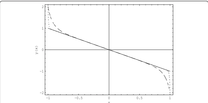
The asymptotic solution (43) is simulated in Figure 1 with different values of ε. In the figure, the solid, dashing, and dotted lines represent, respectively, the reduced solu-tion, the asymptotic solutions with ε= 0.1 andε= 0.01. From this figure, we can see that
(1) delayed phenomenon of loss of stability of solutions really occurs, that is, exis-tence of canards in this boundary value problem is verified. This canard solution is approximated by (43) with the accuracy of zero-order;
-1 -0.5 0 0.5 1
x -2
-1 0 1 2
y
x
(2) with ε®0, the asymptotic solution approaches more and more to the reduced solution in the whole interval (a,b). Therefore, the zero-order approximation is suffi-ciently accurate for the small ε.
Authors’contributions
The authors wrote this article in collaboration and with same responsibility. All authors read and approved the final manuscript.
Competing interests
The authors declare that they have no competing interests.
Received: 6 March 2011 Accepted: 14 October 2011 Published: 14 October 2011
References
1. Kevorkian, JK, Cole, JD: Perturbation Methods in Applied Mathematics. Springer, New York (1981)
2. Verhulst, F: Methods and Applications of Singular Perturbations: Boundary Layers and Multiple Timescales Dynamics. Springer, New York (2005)
3. Tikhonov, AN: On the dependence of solutions of differential equations on a small parameter. Math. Sb.73, 575–586 (1952)
4. Tikhonov, AN: Systems of differential equations containing a small parameter. Math. Sb.64, 193–204 (1948) 5. Fenichel, N: Geometric singular perturbation theory for ordinary equations. J. Diff. Equs.31, 53–98 (1979) 6. Christopher, KRT: Geometric singular perturbation theory. Lecture Notes Math.1609, 44–118 (1995)
7. Lin, XB: Heteroclinic bifurcation and singularly perturbed boundary value problems. J. Diff. Equs.84, 319–382 (1990) 8. Beck, M, Doelman, A, Kaper, TJ: A geometric construction of traveling waves in a bioremediation model. J. Nonlinear
Sci.16, 329–349 (2006)
9. Hek, G: Geometric singular perturbation theory in biological practice. J. Math. Biol.60, 347–386 (2010)
10. Butuzov, VF, Nefedov, NN, Schneider, KR: Singularly perturbed problems in cases of exchange of stabilities. J. Math. Sci. 1210, 1973–2079 (2004)
11. Callot, JL, Diener, F, Diener, M: Le Problème de la“chasse au canard”. C. R. Acad. Sci. Paris.286, 1059–1061 (1978) 12. Eckhaus, W: Relaxation oscillations including a standard chase on French ducks. Lecture Notes Math.985, 449–494
(1983)
13. Xie, F, Han, M, Zhang, W: Canard phenomena in oscillations of a surface oxidation reaction. J. Nonlinear Sci.15, 363–386 (2005)
14. Horacio, G.,et al: A Canard mechanics for localization in systems of globally coupled oscillators. SIAM J. Appl. Math.63, 1998–2019 (2003)
15. O’Malley, RE Jr: Singular Perturbation Methods for Ordinary Differential Equations. Springer, New York (1991) 16. Lin, P, O’Malley, RE Jr: The numerical solution of a challenging class of turning problems. SIAM J. Sci. Comput.25,
927–941 (2003)
17. Shchepakina, E, Sobolev, V: Integral manifolds, canards and black swans. Nonlinear Anal. TMA.44, 897–908 (2001) 18. Chang, KW, Howes, FA: Nonlinear Singular Perturbation Phenomena: Theory and Application. Springer, New York (1983)
doi:10.1186/1687-2770-2011-35
Cite this article as:Zhou and Shen:Delayed phenomenon of loss of stability of solutions in a second-order
quasi-linear singularly perturbed boundary value problem with a turning point.Boundary Value Problems2011 2011:35.
Submit your manuscript to a
journal and benefi t from:
7Convenient online submission
7 Rigorous peer review
7Immediate publication on acceptance
7 Open access: articles freely available online
7High visibility within the fi eld
7 Retaining the copyright to your article