Department of Mathematics
Doctoral School in
Mathematics
C
omplexity in
I
nfinite
G
ames on
G
raphs
and
T
emporal
C
onstraint
N
etworks
D
octoral
D
issertation
Author
Carlo Comin
Advisor
Co-Advisor
Complexity in Infinite Games on Graphs
and Temporal Constraint Networks
A dissertation
presented to the Doctoral School in Mathematics
of the University of Trento
in partial fulfilment of the requirements for the
Ph.D. Degree
Sous la co-tutelle de
LIGM, Universit´e Paris-Est Marne-la-Vall´ee
by
Carlo Comin
January 2017
Advisor
Co-Advisor
Prof. Romeo Rizzi
D.d.R. St´ephane Vialette
University of Verona, Italy Universit`e Paris-Est Marne-la-Vall´ee, France
Referee
Referee
Prof. Luke Hunsberger
Prof. Angelo Montanari
Abstract
This dissertation deals with a number of algorithmic problems motivated by automated temporal planning and formal verification of reactive and finite state systems. Particularly, we shall focus on game theoretical methods in order to obtain improved complexity bounds and faster algorithms.
In thefirst paperwe introduceHyper Temporal Networks (HyTNs), a strict gen-eralization of Simple Temporal Networks (STNs), to overcome the limitation of considering only conjunctions of constraints but maintaining a practical effi-ciency in the consistency check of the instances. STNs provide a powerful and general tool for representing conjunctions of maximum delay constraints over ordered pairs of temporal variables. HyTNs are meant as a light generalization of STNs offering an interesting compromise. On one side, there exist practical pseudo-polynomial time algorithms for checking consistency and computing feasible schedules for HyTNs; the computational equivalence between check-ing consistency in HyTNs and determincheck-ing winncheck-ing regions in Mean Payoff Games (MPGs) is also pointed out. On the other side, HyTNs offer a more powerful model accommodating natural constraints that cannot be expressed by STNs like“Trigger off exactlyδmin before (after) the occurrence of the first (last) event in a set.”
Then, we turn our attention to the Conditional Simple Temporal Network (CSTN) model, a constraint-based graph-formalism for conditional temporal planning. Three notions of consistency arise for CSTNs: weak, strong, and dynamic. Dynamic consistency is the most interesting notion, but it is also the most challenging and it was conjectured to be hard to assess. CSTNs are an extension of Simple Temporal Networks (STNs) [44]. In the second paper we introduce and study theConditional Hyper Temporal Network (CHyTN)model, a natural extension and generalization of both the CSTN and the HyTN model, obtained by blending them together. We show that deciding whether a CSTN is dynamically-consistent iscoNP-hard; and that deciding whether a CHyTN is dynamically-consistent isPSPACE-hard, when the input instances are allowed to include both multi-head and multi-tail hyperarcs. Then, we offer the first deterministic (pseudo) singly-exponential time algorithm for the problem of checking the dynamic consistency of such CHyTNs, also producing a dynamic execution strategy whenever the input CHyTN is dynamically-consistent. The presentation of such connection is mediated by the HyTN model. In order to analyze the time complexity of the algorithm, we introduce a refined notion of dynamic consistency, namede-dynamic consistency, and present a sharp lower
transits from being, to not being, dynamically-consistent.
Theε-DC notion turns out to be interesting per se, and the proposedε
-DC-Checking algorithm rests on the assumption that reaction-time satisfies ε>0;
leaving unsolved the question of what happens whenε=0. In thethird paper,
we introduce and study π-DC, a sound notion of DC with an instantaneous reaction-time(i.e., one in which the planner can react to any observation at the same instant of time in which the observation is made). Firstly, we demon-strate by a counter-example that π-DC is not equivalent to 0-DC, and that
0-DC is actually inadequate for modeling DC with an instantaneous reaction-time. This shows that our previous results do not apply directly, as they were formulated, to the case ofε=0. Then, our previous tools are extended in order
to handleπ-DC, and the notion ofps-treeis introduced, also pointing out a
re-lationship betweenπ-DC and HyTN-Consistency. Thirdly, a simple reduction
from π-DC to DC is identified. This allows us to design and to analyze the
first sound-and-complete π-DC-Checking procedure, whose time complexity
remains (pseudo) singly-exponential in the number of propositional letters. Next, an arena is a finite directed graph whose vertices are divided into two classes, i.e.,V=V∪V#; this forms the basic playground for a plethora of 2-player infinite pebble games. In thefourth paper, we introduce and study a re-fined notion of reachability for arenas, namedtrap-reachability, where Player attempts to reach vertices without leaving a prescribed subset U⊆V, while Player#works against. It is shown that every arena decomposes into strongly-trap-connected components (STCCs). Our main result is a linear time algorithm for computing this unique decomposition. This theory has direct applications in solving Update Games (UGs) faster. Dinneen and Khoussainov showed in 1999 that deciding who’s the winner in a given UG costsO(mn)time, where
n is the number of vertices and m is that of the arcs. We solve that problem inΘ(m+n)linear time. Finally, the polynomial-time complexity for deciding Explicit McNaughton-M ¨uller Games is also improved, from cubic to quadratic. Then, in the fifth paper we offer a Θ(|V|2|E|W) pseudo-polynomial time
and Θ(|V|)space deterministic algorithm for solving the Value Problem and Optimal Strategy Synthesis in Mean Payoff Games. This improves by a factor log(|V|W) the best previously known pseudo-polynomial time upper bound of Brim,et al. In thesixth paperwe further strengthen the links between Mean Payoff Games (MPGs) and Energy Games (EGs). We offer a fasterO(|V|2|E|W)
pseudo-polynomial time and Θ(|V|+|E|) space deterministic algorithm for solving the Value Problem and Optimal Strategy Synthesis in MPGs. This improves significatly over our previous Θ(|V|2|E|W)time algorithm, also in
practice. Moreover, we study structural aspects concerning Optimal Positional Strategies (OPSs) in MPGs. We observe aunique complete decomposition of the space of all OPSs,optΓΣM0 , in terms of so-calledextremal-SEPMs in reweighted Energy Games; this points out what we called the “Energy-Lattice XΓ∗ of
Acknowledgements
First and foremost I wish to thank my thesis advisor, Prof. Romeo Rizzi, for his guidance and for the time and efforts he dedicated to my training during this journey. He has been a constant source of friendly support and inspiration without whom this thesis would not exist. Romeo has been the greatest mentor from all points of view.
I was lucky and honored to have been one of his students.
I wish to thank my co-advisor,D.d.R. St´ephane Vialette, for supporting me at UPEM and for having accompanied me throughout my stay in France. I came into contact with an outstanding research environment and with the best research seminars I had ever experienced. I also thank him for his advices which supported my path.
I wish to thank the external referees of this dissertation,Prof. Luke Hunsbergerand
Prof. Angelo Montanari, as well asDr. Pietro Sala andDr. Nicola Gigante, for their careful review and for their valuable comments which helped improving both the content and quality of the manuscript.
I thank Dr. Anthony Labarrefor kindly sharing with me his office at UPEM for a period of time and for having worked together during my stay and later on.
Thanks to theAlgoB Groupat UPEM,Dr. Philippe Gambette,Dr. Karel Bˇrinda,
Dr. Emerite Both Neou, as well asDr. Massimo Cairoand all the Doctoral Fellows of the XXIX cycle in Maths at University Trento, for making this unique experience and for being great and friendly colleagues.
Lastly, I would like to thank my family for all their love and encouragement.
A special thank goes to my mother, words cannot express all the sacrifices she has made on my behalf. I hope one day to be able to make a sense of all these.
Contents
1 Introduction and Context 5
1.1 Contributions and Organization . . . 6
1.2 Constraint Satisfaction Problems . . . 8
1.2.1 Temporal Constraint Networks . . . 10
1.2.2 Simple Temporal Networks . . . 11
1.3 Algorithmic Game Theory . . . 13
1.3.1 Topological Banach-Mazur Games . . . 14
1.3.2 Gale-Stewart Games . . . 15
1.3.3 Borel Determinacy Theorem . . . 16
1.4 Modal µ-calculus, ω-Regular and Mean-Payoff Games . . . 17
1.4.1 Syntax and Semantics of the Modalµ-calculus . . . 17
1.4.2 ω-Regular Games . . . 21
1.4.3 From model-checking ofLµ to parity games . . . 25
1.4.4 Mean-payoff games . . . 27
1.4.5 From parity games to mean-payoff games . . . 28
I Temporal Constraint Networks 29 2 Hyper Temporal Networks 30 2.1 Introduction . . . 31
2.1.1 Contribution . . . 32
2.1.2 Organization . . . 32
2.2 Motivating Examples . . . 32
2.3 Background and Notation . . . 38
2.4 HyTN and Consistency Property . . . 39
2.5 Mean Payoff Games . . . 47
2.6 The Reductions . . . 51
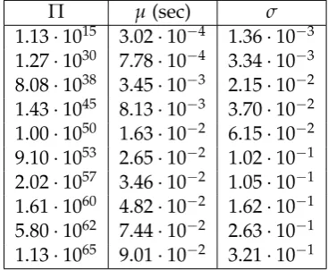
2.7 Computational Experiments . . . 60
2.8 Related Works . . . 70
3 Checking Dynamic Consistency of Conditional Hyper Temporal
Net-works via Mean Payoff Games 74
3.1 Introduction and Motivation . . . 76
3.1.1 Contribution . . . 77
3.1.2 Organization . . . 79
3.2 Background and Notation . . . 79
3.2.1 Simple Temporal Networks . . . 79
3.2.2 Hyper Temporal Networks . . . 79
3.3 Conditional Simple / Hyper Temporal Networks . . . 80
3.4 Algorithmics of Dynamic Consistency . . . 87
3.4.1 e-Dynamic Consistency . . . 95
3.4.2 A (pseudo) Singly-Exponential Time Algorithm for DC and CHyTN-DC . . . 99
3.5 Bounding Analysis on the Reaction Time ˆe . . . 105
3.6 Related Works . . . 112
4 Instantaneous Reaction-Time in Dynamic Consistency Checking of Conditional Simple Temporal Networks 114 4.1 Introduction and Motivation . . . 115
4.1.1 Contribution . . . 115
4.2 Background and Notation . . . 116
4.2.1 ε-Dynamic-Consistency . . . 116
4.3 DC with Instantaneous Reaction-Time . . . 117
4.3.1 The ps-tree: “skeleton” structure forπ-dynamicπ-ESs . . 121
4.3.2 Verifying a c-ps-tree. . . 123
4.3.3 A Singly-Exponential Timeπ-DC-Checking Algorithm . . 127
4.4 Related Works . . . 132
4.5 Conclusion . . . 133
II Infinite Games on Graphs 134 5 Linear Time Algorithm for Update Games via Strongly-Trap-Connected Components 135 5.1 Introduction . . . 136
5.1.1 Background and Notation . . . 137
5.2 Trap-Reachability . . . 137
5.3 Strongly-Trap-Connectedness . . . 140
5.4 TR-Depth-First-Search . . . 142
5.5 Linear Time Algorithm for STCCs . . . 154
5.5.1 Proof of Correctness of Algo. 13 . . . 161
5.6 Application to Update Games . . . 163
5.7 Application to Explicit McNaughton-M ¨uller Games . . . 165
6 Improved Pseudo-Polynomial Upper Bound for the Value Problem
and Optimal Strategy Synthesis in Mean Payoff Games 166
6.1 Introduction . . . 167
6.1.1 Contribution . . . 168
6.1.2 Organization . . . 169
6.2 Background and Notation . . . 169
6.3 Values and Optimal Positional Strategies from Reweightings . . . 175
6.3.1 On Optimal Values . . . 175
6.3.2 On Optimal Positional Strategies . . . 178
6.4 A Θ(|V|2|E|W) time Algorithm for solving the Value Problem and Optimal Strategy Synthesis in MPGs . . . 183
6.4.1 Description of the Algorithm . . . 184
6.4.2 Proof of Correctness . . . 188
6.4.3 Complexity Analysis . . . 192
6.5 Conclusions . . . 194
7 FasterO(|V|2|E|W)-Time Energy Algorithm for Optimal Strategy Syn-thesis in Mean Payoff Games 195 7.1 Introduction . . . 196
7.1.1 Contribution . . . 196
7.1.2 Organization . . . 197
7.2 Background and Notation . . . 198
7.3 A Faster O(|V|2|E|W)-Time Algorithm for MPGs by Jumping through Reweighted EGs . . . 198
7.3.1 Description of Algorithm 15 . . . 199
7.3.2 Correctness of Algorithm 15 . . . 218
7.3.3 Complexity of Algorithm 15 . . . 238
7.3.4 An Experimental Evaluation of Algorithm 15 . . . 239
7.4 Conclusion . . . 242
8 The Energy Structure of Optimal Positional Strategies in MPGs 243 8.1 Introduction . . . 245
8.1.1 Contribution . . . 245
8.1.2 Organization . . . 246
8.2 An Energy-Lattice Decomposition ofoptΓΣM0 . . . 246
1
Introduction and Context
This dissertation provides further evidence that game theoretic arguments help to study algorithmic problems in the area of automated temporal planning and formal verification of finite state non-terminating systems.
Automated temporal planning[44, 59, 88] is a branch of Artificial Intelligence (AI) that concerns the realization of temporal strategies or temporal action se-quences, typically for execution by intelligent agents, autonomous robots and unmanned vehicles. Unlike classical control and classification problems, the solutions are complex and must be discovered and optimized in multidimen-sional space. Planning is also related to decision theory. In known environ-ments with available models, planning can be done offline; solutions can be found and evaluated prior to execution. In dynamically unknown environ-ments, the strategy often needs to be revised online; solutions usually resort to iterative trial and error processes commonly seen in AI.
On the other hand,non-terminatingcomputing systems involving multiple, distributed, and interacting agents [106, 119] abound today and can be found in environments as varied as household appliances, medical equipment, in-dustrial control systems, flight control systems in airplanes, etc. In these con-texts, failures caused by design faults may be very costly and they should be avoided as much as possible. Behaviour of such systems is typically very complex which makes their design and validation a challenge. Formal methods
try to address this challenge by developing formal models of such systems, and methods to specify and reason about their properties. A formal method is of particular interest if it offers not only a rigorous and unambiguous way to describe systems and their intended behaviour, but also provides efficient algorithms allowing to automate (parts of) the design and validation tasks.
We began our research by studying algorithmic problems in automated temporal planning, particularly, our original motivation was the study of cer-tainconditionaltemporal planning problems. At some point, we have identified interesting connections between the algorithmics of these problems and that of some fundamental tasks related to a specific family of infinite 2-player pebble games that are played on finite graphs, i.e., the Mean Payoff Games (MPGs). These games, in addition to being of an independent interest, are intimately related to the semantics of a well-known model of calculus for formal verifica-tion, e.g., the modalµ-calculus. In summary, it turned out that a game theoretic
formulation helps to abstract away from syntactic and semantic peculiarities of modelling formalisms and makes the conditinal temporal constraints problems in question more easily amendable to algorithmic and complexity analysis.
those conditional temporal planning problems, ultimately obtaining faster al-gorithms and improved complexity bounds; and then, on the other side, these first encouraging results have led us to deepen the study of algorithmic and complexity issues in infinite games on finite graphs per se. In the end, we obtained faster algorithms and improved complexity bounds for some of these games, i.e., Update Games, Explicit McNaughton-M ¨uller Games, and finally, for Mean Payoff Games. Our contributions have thus an algorithmic nature, fo-cused on improving state-of-the-art computational complexity upper bounds.
1.1
Contributions and Organization
This dissertation comprises an introductory chapter and then two major parts. Chapter 1 provides context and background notions on the covered subjects, plus an outline of the main contributions (see below).
Part I presents our contributions in automated temporal planning, it con-tains a revised version of the following articles:
• Carlo Comin, Roberto Posenato, Romeo Rizzi. A Tractable General-ization of Simple Temporal Networks and its relation to Mean Payoff Games. Accepted in21st International Symposium on Temporal Representa-tion and Reasoning (TIME 2014). University of Verona, Verona, Italy. Septem-ber 2014.[32]
• Carlo Comin, Roberto Posenato, Romeo Rizzi. Hyper Temporal Net-works. Accepted in Constraints, an International Journal, Springer-US, pp 1-39. March 2016.[33]
• Carlo Comin, Romeo Rizzi. Dynamic Consistency of Conditional Sim-ple Temporal Networks via Mean Payoff Games: a Singly-Exponential Time DC-Checking. Accepted in22nd International Symposium on Tempo-ral Representation and Reasoning (TIME 2015), University of Kassel, Kassel, Germany. September 2015.[34]
• Carlo Comin, Romeo Rizzi. Checking Dynamic Consistency of Con-ditional Hyper Temporal Networks via Mean Payoff Games (Hardness and pseudo-Singly-Exponential Time Algorithm). Accepted in Informa-tion and ComputaInforma-tion, Elsevier. (It will appear during 2017)[40]
• Massimo Cairo, Carlo Comin, Romeo Rizzi. Instantaneous Reaction-Time in Dynamic-Consistency Checking of Conditional Simple Temporal Networks. Accepted in23rd International Symposium on Temporal Represen-tation and Reasoning (TIME 2016), Technical Univeristy of Denmark (DTU), Copenhagen, Denmark, October 2016.[17]
• Carlo Comin, Romeo Rizzi. Linear Time Algorithm for Update Games via Strongly-Trap-Connected Components (A 2-Player Infinite Pebble Game Generalization of Strongly-Connected Components). Submitted. [39]
• Carlo Comin, Romeo Rizzi. Energy Structure and Improved Complexity Upper Bound for Optimal Positional Strategies in Mean Payoff Games. Accepted in 3rd International Workshop on Strategic Reasoning (SR 2015), University of Oxford, Oxford, U.K., September 2015.[35]
• Carlo Comin, Romeo Rizzi. Improved Pseudo-Polynomial Bound for the Value Problem and Optimal Strategy Synthesis in Mean Payoff Games. Accepted inAlgorithmica, Springer-US, pp 1-27, February 2016.[38]
• Carlo Comin, Romeo Rizzi. FasterO(|V|2|E|W)-Time Energy Algorithm
for Optimal Strategy Synthesis in Mean Payoff Games. Submitted. [37]
During the doctoral course, the author of this dissertation also co-authored the following articles; which however do not belong to this dissertation, being motivated by topics in computational biology.
• Carlo Comin, Anthony Labarre, Romeo Rizzi, St´ephane Vialette. Sorting with Forbidden Intermediates. Accepted in 3rd International Conference on Algorithms for Computational Biology (AlCoB 2016), Trujillo, Spain. June 2016 [31]. An extended version of this paper has been submitted to the
IEEE/ACM Transactions on Computational Biology and Bioinformatics.
• Carlo Comin, Romeo Rizzi. An Improved Upper Bound on Maximal
Clique Listing via Rectangular Fast Matrix Multiplication. Accepted in Algorithmica, Springer-US. (It will appear during 2017)[36]
For completeness, we mention another published contribution related to the theory of automata; but the result contained in the article below has not been obtained during the doctoral course, it belongs to author’s MSc thesis.
• Carlo Comin. Algebraic Characterization of the Class of Languages Rec-ognized by Measure Only Quantum Automata. Accepted inFundamenta Informaticae, Annales Societatis Mathematicae Polonae, IOS Press, 335–353, vol 134, 2014.[29]
1.2
Constraint Satisfaction Problems
The notion of constraint is central to a number of human activities and dis-parate processes. A constraint limits (or restricts) the field of possibilities in a certain universe. For example, a school timetable that coordinates students, teachers, lessons, rooms and time slots, must satisfy many constraints, i.e., not all combinations are possible since the involved constraints may be numerous and various. Besides school timetabling, constraint satisfaction problems arise in many enterprise and industrial tasks, ranging from scheduling to configu-ration, circuit design and molecular biology [78]. Also in Artificial Intelligence (AI) and Operations Research (OR),constraint satisfactionis the process of find-ing a solution to a set of constraints imposfind-ing conditions that the variables must satisfy. A solution is therefore a set of values for the variables that sat-isfies all the constraints – that is, a point in the feasible region. Formally, we shall consider the following model:
Definition 1.1([101]). Aconstraint satisfaction problem (CSP)is a triplet,
Φ,(X,D,C),
where:
• X,{X1,X2, . . . ,Xn}is a set of variables;
• D,{D1,D2, . . . ,Dn}is a set of nonempty domains;
• C,{C1,C2, . . . ,Cm}is a set of constraints.
Each variable Xi will take on its value in the nonempty domain Di, i.e., Di is the domain of possibles values of Xi. Each constraint Cj involves some subset of the variables and specifies the allowable combination of values for that subset, i.e., Cj is in turn a pair(Tj,Rj)where Tj⊆X is a subset of k variables and Rj is a k-ary relation on the corresponding subset of domains. A state Ψ of the CSP Φ is defined by an assignment of values to some or all of the variables, i.e.,
Ψ,{Xi=vi,Xj=vj, . . .}, for some vi∈Di,vj∈Dj, . . .
An assignment that doesn’t violate any constraint isconsistent (orfeasible), where a constraint (Tj,Rj)issatisfied if the values assigned to the variables Tj satisfy the relation Rj. Acompleteassignment is one in which every variable is mentioned, and asolutionto a CSP is a complete assignment that satisfies all the constraints.
Notable examples of problems that can be modeled as a CSP include the
eight queens puzzle.
Example 1.1. This is the problem of placing eight chess queens on an8×8chessboard
to find out only which row each of these queens is going to be placed in. Thus we have8variablesX,{Q1,Q2, . . . ,Q8}, each of which can assume the value within the domain Di,{1, . . . , 8}. Given that a feasible solution is a configuration in which no two queens can attack each other, we have the following constraints: horizontally, no two queens should be in the same row, so:
Qi 6=Qj whenever i6=j;
along any diagonal, they should not be the same number of columns apart as they are rows apart, so:
|Qi−Qj| 6=|i−j|whenever i6=j.
Thus there are56constraints. Of course the puzzle can be generalized, with n queens on a chessboard of n×n squares (the reader is referred to e.g. [3] for a survey of known results and research open problems concerning the n-queens puzzle).
The identification of CSPs as a general class is due to Ugo Montanari [88], who also pointed out the notion of constraint network and propagation by path consistency. Recall that a n-ary relation over the variablesX1,X2, . . . ,Xn is any
subset of the corresponding domainsD,D1×D2×. . .×Dn. Let us denote by Rij any binary relation betweenXi andXj, where we allow Rij6=Rjigenerally.
Giveni∈[n], the identity relationIiiexists, defined only between a variableXi
and itself, as follows: Iii,{(d,d)|d∈Di}. Also, it is worth mentioning the
unit relation Uii,Di×Di. The formal definition of constraint network(i.e., a
network of binary constraints) goes as follows.
Definition 1.2([88]). Aconstraint networkN ,(D,{Ri,j}i,j)is made of a family
of sets,
D,{D1,D2, . . . ,Dn},
plus a relation Rij from every set Dito every set Dj, for i,j∈ {1, 2, . . . ,n}. Furthermore, Rii⊆Iii for every i.
A constraint network can be thought of as representing a n-ary relation
ρ, where the n-tuple a∈ρ iff its projections on all the two-dimensional
sub-spaces of Dsatisfy the binary constraints of N. A useful way of visualizing a network is by a directed graph in which vertices v1,v2, . . . ,vn correspond to
sets D1,D2, . . . ,Dn, and an arc (vi,vj) is present iff Rij 6=Uij (when i6= j) or Rii6=Iii [88]. For instance,
Example 1.2. The following n-ary (n=3) relationρis represented by the network in
Fig. 1.1; let Di={xi1,xi2,xi3}for i=1, 2, 3, then let:
ρ,{(x11,x21,x31),(x11,x21,x32),(x12,x23,x31)}.
v1
v3
v2
Figure 1.1: The constraint networkρof Example 1.2.
1.2.1 Temporal Constraint Networks
In [44], network-based methods of constraint satisfaction are extended to in-clude continuous variables, thus providing a framework for processing tem-poral constraints.
Definition 1.3 ( [44]). A temporal constraint network (TN) Γ is a constraint
network involving a set of variables X,{X1,X2, . . . ,Xn} having continuous (real-valued) domains D,{D1,D2, . . . ,Dn}; each variable represents a time point. Fur-thermore, a setCof unary and binary constraints is involved. Each (unary or binary) constraint Cj∈Cis represented by a set of real intervals:
Cj,{I1,I2, . . . ,Ik}=
[a1,b1],[a2,b2], . . . ,[ak,bk] .
Closed, open and semi-open intervals are generally allowed. The intended interpreta-tion going as follows.
• A unary constraint Tii restricts the domain of variable Xi to the given set of intervals; namely, it represents the disjunction:
k _
q=1
aq≤Xi≤bq
.
• Abinaryconstraint Tij constrains the permissible values for the distance Xj− Xi; namely, it represents the disjunction:
k _
q=1
aq≤Xj−Xi ≤bq
.
Constraints are given in acanonical formwhere all intervals are pairwise disjoint.
A TN can be represented by a directed constraint graph, in much the same way as we did above for constraint networks, where vertices represent vari-ables and an arc (Xi,Xj)indicates that a proper constraint Tij is specified; but
X1
X3
X2 [a
1,b 1],[
a2 ,b
2] [c
1,d 1],[
c2 ,d
2]
[e1,f1 ],[e2,
f2], [e3,f3
]
[g1,h1]
Figure 1.2: A Temporal Constraint Network.
Usually, a special time point Z(or X0) is employed to represent the
begin-ning of the world, i.e., for simplicity Zis always scheduled at timetZ=0. All
other times are relative to Z; thus we may treat each unary constraint Tii as a
binary constraint T0i (having the same interval representation).
1.2.2 Simple Temporal Networks
Definition 1.4. Asimple temporal problem (STP)(orsimple temporal network
(STN)) is a TN in which all constraints specify a single interval; namely, for each constraint Cj, there is an interval Ij such that Cj={Ij}.
In STNs, each arc(Xi,Xj)is labeled by an interval[aij,bij], representing the
constraint:
aij ≤Xj−Xi≤bij.
Alternatively, the same constraint can be expressed as a pair of inequalities:
Xj−Xi≤bij andXi−Xj≤ −aij
Notice that solving a STP/STN amounts to solving a set of linear inequalities on theXi, where each inequality involves exactly two variables; thus a
shortest-path algorithm on graphs, such as Bellman-Ford [4, 42, 55], can be applied. Particularly, we shall consider graphs that are directed and weighted on the arcs. Thus,
Definition 1.5. If G= (V,A)is a graph, then every arc a∈A is a triple(ta,ha,wa)
where ta∈V is the tail of a, ha∈V is the head of a, and wa∈Ris the weight of a. Moreover, since we use graphs to represent distance constraints, they do not need to have either loops (unary constraints are meaningless) or parallel arcs (two parallel constraints represent two different distance constraints between the same pair of node: only the most restrictive is meaningful). We also use the notations h(a) for ha, t(a) for ta, and w(a)or w(ta,ha)for wa, when it helps.
The order and size of a graph G= (V,A)are denoted by
respectively. The size is a good measure for the encoding length of G.
Definition 1.6. Acycleof G is a set of arcs C⊆A cyclically sequenced as a0,a1, . . . ,a`−1
so that,
h(ai) =t(aj) ⇐⇒ j= (i+1) mod`;
it is called anegative cycleif w(C)≤0, where w(C)stands for∑e∈Cwe.
Definition 1.7. A graph is called conservative when it contains no negative cycle.
A potential is a function p:V7→R. The reduced weight of an arc a= (u,v,wa) with respect to a potential p is defined as
wap,wa−pv+pu.
A potential p of G= (V,A)is called feasible if wap≥0for every a∈A. Notice that, for any cycle C, wp(C) =w(C). Therefore, the existence of a feasible potential implies that the graph is conservative as w(C) =wp(C)≥0for every cycle C.
So, the Bellman-Ford algorithm [4, 42, 55] can be used to produce inO(nm)
time:
• either a proof thatGis conservative in the form of a feasible potential;
• or a proof that G is not conservative in the form of a negative cycle C
inG.
When the graph is conservative, the smallest weight of a walk between two nodes is well defined, and, fixed a root noder inG, the potentials returned by the Bellman-Ford algorithm are, for each nodev, the smallest weight of a walk fromr to v. Moreover, if all the arc weights are integral, then these potentials are integral as well. Therefore, the Bellman-Ford algorithm provides a proof to the following theorem.
Theorem 1.1 ([4, 42, 55]). A graph admits a feasible potential if and only if it is
conservative. Moreover, when all arc weights are integral, the feasible potential is an integral function.
Thus an STN can be viewed as a weighted graph whose nodes are time-points that must be placed on the real line and whose arcs express mutual constraints on the allocations of their end points.
Definition 1.8. An STN G= (V,A) is called consistent if it admits a feasible
scheduling, i.e., a scheduling s:V7→Rsuch that
s(v)≤s(u) +w(u,v), ∀arc(u,v)of G.
Then we have the following characterization result for STN’s consistency in terms of conservative graphs.
Proof. A feasible scheduling is just a feasible potential. Therefore, this
corol-lary is just a restatement of Theorem 1.1. 2
The reader is referred to [44] for further details and fundamental properties concerning the theory of TNs and STNs.
1.3
Algorithmic Game Theory
As argued in [120], the birth ofAlgorithmic Game Theory (AGT)is often equated with the following three seminal papers, cited in [56] for laying the foundation of growth in AGT:
• Koutsoupias, Papadimitriou, Worst-case Equilibria. STACS 1999: 404-413[74], introduced the notion of “price of anarchy”, a measure of the extent to which competition approximates cooperation, quantifying how much utility is lost due to selfish behaviors on the Internet, which operates without a system designer or monitor striving to achieve the social opti-mum.
• Roughgarden, Tardos: How Bad is Selfish Routing? FOCS 2000: 93-102[100], studied the power and depth of the “price of anarchy” as it applies to routing traffic in large-scale communications networks to optimize the performance of a congested network.
• Nisan, Ronen: Algorithmic Mechanism Design. STOC 1999: 129-140 [91], studied classical mechanism design from algorithmic and complexity-theoretic perspectives.
However the study of algorithmic questions in combinatorial games goes back a long time ago. Perphaps the first combinatorial game described in a math-ematical form (in Europe) dates back to the beginning of the XVII century, to the time whenBachet de M´eziriacproposed in his“Probl´emes Plaisants” the fol-lowing game: two players alternately choose numbers between 1 and 10; the player, on whose move the sum attains exactly 100, is the winner. This kind of game, whose natural generalization nowadays is known as Nim, was also studied by Bouton (1901-2) [11]and it has an extensive literature [6]. In Nim, under the normal play convention, the game is between two players and it is played with n heaps (i.e., a pile of n counters) of any number of objects. The two players alternate by taking (removing), at each turn, any number of objects from any single one of the heaps at their choice. The winning condition is to be the last to take an object. So, Nim can be played as anormal play game, i.e., one in which the player who makes the last move wins. Also, Nim isimpartial
which asserts that every impartial game under the normal play convention is equivalent to animber(i.e., the value of a Nim heap of a certain size) [41].
The nimbersare the ordinal numbers,
0, 1, 2, . . . ,n, . . . ,ω,ω+1,ω+2, . . . ,ω·2,ω·2+1,ω·2+2, . . . ,ω2, . . . ,ω3, . . . ,ωω, . . . ,ωω
ω , . . .
endowed with a new nimber additionandnimber multiplication, which are dis-tinct from ordinal addition and ordinal multiplication; see [41] for more de-tails. Some other connections between positional games and the infinite soon emerged in the literature.
1.3.1 Topological Banach-Mazur Games
The infinite positional games of perfect information were discovered and ini-tially studied in Poland around the ’30s. In 1935Stefan Banach started a note-book, called theScottish Book, where the mathematicians residing in or visiting Lw ´ow proposed various mathematical problems, or conjectures, and also in-dicated their partial or complete solutions. In the same year Stanisław Mazur
proposed an infinite combinatorial game. The game is described in Problem 43 of the Scottish Book; its solution, given by Banach, is dated August 4, 1935. Hence, the game became known as theBanach-Mazur Game. Mazur discovered the game in 1928; however, later on,Ulam[114] gives the year 1935 for its com-plete solution, referring to a conversation in the Scottisch Caf´e, where “Mazur proposed the first examples of infinite mathematical games”). Later on Ulam prepared an English translation of the Scottish Book, see [115].
Definition 1.9(Banach-Mazur Games onR). In aBanach-Mazur Game, played
on the real line, the winning condition is given by a setWin⊆Rof real numbers; in the first move, Player 0 selects an interval d0on the real line, then Player 1 chooses an interval d1(d0, then Player 0 chooses a further refinement d2(d1and so on. Thus a play forms an infinite (proper) chain sequence:
d0)d1)d2)· · ·.
Player 0 wins iff the intersection of all intervals di contains a point ofWin; namely,
Player 0 wins ⇐⇒ \
n∈N
dn∩Win6=∅.
A similar game can be played on a generic topological spaceX. LetV be a family of subsets ofX such that: each V∈Vcontains a nonempty open subset of X; and each nonempty open subset of Xcontains an element V∈V. In the Banach-Mazur game defined on(X,V)with winning condition W⊆X, the two players take turns to choose sets V0)V1)V2)· · · inV, where Player 0 wins iffTn∈NVn∩Win6=∅.
Definition 1.10(Determinacy). A game is said to bedeterminedif one or the other
Concerning the determinacy of these games, the original proof of Banach never appeared. The first published proof is that ofOxtoby Theorem[94], which characterizes determinacy oftopological Banach-Mazur games in terms of topo-logical properties of the winning condition. The term “topological game” was introduced by Berge [5].
Observe that Banach-Mazur’s infinite game can also be played on graphs:
Definition 1.11(Banach-Mazur Games on Graphs). It is given(G,vs), where G=
(V,A)is a directed graph and vs∈V is a distinguished initial vertex, it is assumed that G has no sink vertices. A winning conditionWinis any subset of infinitely long paths in G, each starting at v, i.e., anyWin⊆Paths(G,vs). The game(G,vs,Win) starts at vertex vs with a move of Player 0 and the players strictly alternate. In a move, after a sequence of moves p0,p1, . . . ,pm−1 forming a finite path, p0p1· · ·pm−1, that has already been played, the corresponding Player (i mod 2)prolongs the path by choosing another finite path pi whose initial vertex is the end vertex of pm−1. Thus, a play results into an infinite path:
π,p0p1· · ·pm· · · ∈Paths(G,v),
the winning condition being that:
Player 0 wins ⇐⇒ π∩Win6=∅;
otherwise, Player 1 wins.
This reformulation shows that Banach-Mazur games are an interesting starting point for the exploration of properties of infinite games on graphs. Many infinite games on graphs and their determinacy properties find a natu-ral place in a hierarchy known as the Borel Hierarchy, whereas the fundamen-tal theorem concerning determinacy in infinite games is theBorel Determinacy Theorem; the latter can be formulated in terms ofGale-Stewart Gameswhich are recalled in the next subsection.
1.3.2 Gale-Stewart Games
In 1953David Gale andFrank Stewartintroduced the following positional infi-nite game of perfect informationin [57]. This allowed them to observe fruitful connections between set theory and infinite games, particularly, this led to important applications of the notion of determinacy in the foundations of set theory [83, 90].
Definition 1.12(Gale-Stewart Games). LetΣbe analphabet, i.e., a finite nonempty
set of symbols. A Gale-Stewart game on Σis a pairΓ,(Σ,Win), whereWin⊆Σω
singleplayof the game determines an infinite sequence:
π,(a0,a1, . . . ,an, . . .)∈Σω.
At this point, Player 0 wins ifπ∈Win; otherwise, the winner is Player 1.
Definition 1.13(Open Gale-Stewart Games). Given a word p∈Σ∗, the following
subset[p]⊆Σω is named acone:
[p],{π∈Σω|p is a prefix ofπ}. We say that,
U⊆Σω isopen ⇐⇒ every
π∈U has a prefix p such that[p]⊆U.
IfOis the family of all open subsets ofΣω, then(Σω,O)is called theCantor topology
onΣω. A Gale-Stewart gameΓ,(Σ,Win)is calledopen (closed)wheneverWinis
so in the Cantor topology onΣω.
The main result of Gale and Stewart [57] is dated 1953, going as follows.
Theorem 1.2 (Gale-Stewart Determinacy Theorem [57]). Every open or closed
Gale-Stewart game is determined.
In the next twenty years this result was extended to slightly higher levels of the Borel hierarchy. At some point this led to the question of whether or not the Gale-Stewart game is determined whenever the payoff set isBorel, as recalled next.
1.3.3 Borel Determinacy Theorem
The question of whether Borel Gale-Stewart games are determined was an-swered byDonald A. Martin[81] in 1975. Let us firstly recall some basic notions from topology.
Definition 1.14. Let Γ be a topological space. A Borel set is any set in Γ that
can be formed from open sets through the operations of countable union, countable intersection, and relative complement (set difference).
Notice that the collection of all Borel sets of Γ forms a σ-algebra; indeed,
the Borel sets are the smallestσ-algebra of subsets of Σω containing all open
sets inO.
At this point, Borel sets are classified in the “Borel Hierarchy” according to how many times the operations of complement and countable union are required to produce them from open sets.
Definition 1.15. In theBorel Hierarchythere are three classes for every countable
ordinalα>0:
Σ0
α,Π
0
α, and∆
0
α.
• A set S is inΠ0α iff the complement of S is inΣ0α.
• A set S is inΣ0αforα>1iff there exists a sequence of sets A1,A2, . . .such that each Ai is inΠ0αi for someαi<αand A=∪i≥1Ai.
• A set is in∆0α iff it is both inΣ0α andΠ0α.
Definition 1.16. WhenWinisBorel, the Gale-Stewart game(Σ,Win)is calledBorel.
The Borel Determinacy Theorem states that any Borel Gale-Stewart game is determined, meaning that one of the two players will have a winning strategy for the game.
Theorem 1.3 (Borel Determinacy Theorem [81, 82]). Every Borel Gale-Stewart
game is determined.
As already mentioned, this was proved by Martin [81] in 1975. The origi-nal proof was quite complicated, the same author published a shorter purely inductive proof in 1982 [82].
The Borel Determinacy Theorem provides a framework for the determinacy question of a number of distinct but interrelated infinite game models.
Furthermore, the problem of verifying correctness and temporal aspects of non-terminating computing systems involving multiple, distributed, and interacting agents [106] soon led to the study of interesting model-checking questions [22]. Some of these problems turned out to be equivalent to the de-terminacy question for certain infinite games lying at a low level (3rd level) of the Borel Hierarchy, e.g., theparity games[61,122]. Some of these developments are mentioned in the next subsections.
1.4
Modal
µ-calculus,
ω-Regular and Mean-Payoff Games
1.4.1 Syntax and Semantics of the Modalµ-calculus
The modalµ-calculus is an extension of propositional modal logic, particularly,
it is a logic that combines simple modal operators with fixed point operators to provide a form of recursion. Theµ-calculus originates withDana Scott[105]
andJaco de Bakker[43], later on was further developed by Dexter Kozen[75]. It can be viewed as a logic describing properties oftransition systems, i.e., poten-tially infinite graphs with labeled arcs (transitions) and vertices (states). Tran-sitions are labeled with actions drawn from, A,{a,b,c, . . .}, and states are labeled with sets ofpropositions, drawn fromP,{p1,p2, . . .}.
Thus atransition system can be viewed as a tuple:
M,S,{Ra}a∈A,{Pi}i∈N
,
where S is a set of states, Ra ⊆ S×S is a binary relation defining
(s0,s1),(s1,s2), . . . all lying in Ra. Actually, there is a great interest in efficient
solutions of the model-checking and the satisfiability problems of the modal
µ-calculus, see [13] for a survey. The syntax of modal µ-calculus is formally
recalled next.
Definition 1.17(Syntax of the modalµ-calculus [13,75,105]). LetVarbe a
count-able set of varicount-ables (whose meaning will be sets of states). Aformula αof the modal µ-calculus is defined by the following grammar Lµ:
Lµ,X
p
¬p
α∧β
haiα
[a]α
µX.α
νX.α;
where X∈Var, p∈ P, a∈ A, and α,β range over formulas of Lµ. The formulas
µX.αandνX.αare namedfixpointformulas; and the symbolsµandν are theleast andgreatest fixpoint operators, respectively. Disambiguating parentheses are added when necessary, where[a]andhaibind more tightly than boolean operators,µandν bind loosely.
Example 1.3. The formula (sentence)νY. µX.((p∧ haiY)∨ haiX)
can be written as:
νY.µX.(p∧ haiY)∨ haiX.
One may adopt a series of syntactic tricks to simplify the notation: let us write σX.α for µX.αor νX.α; also, to underline the dependency of the value
of a formulaα on a variable X, σX.α(X)stands for σX.α; in any formula like σX.α(X), we say that X is a bound variable; a variable X isfree in a formula α(X)if it is not bound; asentenceis a formula with no free variables occuring
in it; finally, by α[β/X] we denote the result of substituting β for every free
occurrence of X in α. Note one can always make sure that no variable has
at the same time a free and a bound occurrence in a formula, as clearlyσX.α
is equivalent to σY.α[Y/X]; so, w.l.o.g., bound and free variables are always
different. Also, we can require that every variable is bound at most once in a formula. A formula iswell-namedwhen both of the latter two conditions hold. Moreover, we can even ensure that in every formula µX.α(X) the variable X
appears only once inα(X), asσX.σY.α(X,Y)is equivalent toσX.σX.α(X,X).
Let us proceed by recalling the notion ofunfoldingof a formula, which will be useful in the reminder of this section: fix σ∈ {µ,ν}, any fixpoint formula σX.α(X)is equivalent to its unfolding, namely,α(σX.α(X)); indeed, this
equiv-alence follows directly from the definition of the fixpoint operators µand ν.
Note that there is no negation operation in the syntax, just negations of propo-sitions; however, the operation of the negation of a sentence will turn out to be definable.
A meaning of a formula in a transition system is a set of states satisfying the formula, the meaning of a variable will be also a set of states of the transition system.
Given a transition system,
M,S,{Ra}a∈A,{Pi}i∈N
,
and a valuation,
V:Var→2S,
the meaningJαK M
V of a formulaαof Lµis defined by induction on its structure:
• The meaning of any variable X∈VarisJXK M
V ,V(X);
• The meaning of a propositional constant pi ∈ P and its negation ¬pi ∈ P is defined (respectively) by:
JpiK M
V ,Pi andJ¬piK M
V ,S\Pi.
• Conjunction is interpreted as set intersection:
Jα∧βK M V ,JαK
M V ∩JβK
M V .
• Disjunction is interpreted as set union:
Jα∨βK M V ,JαK
M V ∪JβK
M V .
• The meaning ofhaiαis:
JαK M V ,
s∈S| ∃s0∈S Ra(s,s0)∧s0∈JαK M
V ;
• The meaning of[a]αis:
JαK M V ,
s∈S| ∀s0∈S Ra(s,s0)⇒s0 ∈
JαK M
V ;
• Theµ andν constructs are interpreted as fixpoints of operators on sets of for-mulas. A formulaα(X)with free variable X can be seen as an operator on sets of states, mapping a set S0 to the semantics of α when X is interpreted as S0, namely,
S07→JαKMV[S0/X].
By definition this operator is monotonic, thus it has well defined least and great-est fixpoints by Knaster-Tarski’s fixed point theorem [111].
Then, the meaning ofµandνis defined (respectively) by:
JµX.αK M V ,
\n
S0 ⊆S|JαK M
V[S0/X]⊆S0 o
,
JνX.αK M V ,
[n
S0 ⊆S|S0⊆JαK M V[S0/X]
o
Example 1.4. The formulaνY.µX.(p∧ haiY)∨ haiX means:
“p holds infinitely often on some a-path”.
Concerning the negation operator, as mentioned, it can be expressed within
Lµ in a meaningful way, by induction on the structure of the negated
for-mula [13]:
Definition 1.19(Negation operator for the modalµ-calculus [13]).
¬(¬p),p ¬(¬X),X
¬(α∨β),¬α∧ ¬β ¬(α∧β),¬α∨ ¬β
¬haiα,[a]¬α ¬[a]α,hai¬α ¬µX.α(X),νX.¬α(¬X) ¬νX.α(X),µX.¬α(¬X)
When applying this translation to a formula without free variables (i.e., to a sentence), the final result has all variables occurring un-negated, because of the two negations introduced when negating fixpoint expressions.
Thus, the following holds.
Theorem 1.4([13]). For every sentenceαof Lµ, every transition systemMover the
set of states S, and every valuationV:
J¬αK M
V =S\JαK M V .
We should mention that in 1986 Niwi ´nski [92] introduced a hierarchy of fixpoint terms based on the number of alternations between least and greatest fixpoint operators. Also,EmersonandLei[54] defined a similar notion of alter-nation depthof a formula. While most useful properties can be expressed with few fixpoints, it is the nesting of the two types of fixpoints that is the source of both expressive power and algorithmic difficulties; indeed, the modal µ
-calculus can encode most of the other logics used in verification and still the algorithmics is not harder than the others [13].
Let αbe a well-named formula, thus for every bound variableYwe have a
unique subformula σY.βY in α; let’s say thatY is a µ-variable or a ν-variable
depending on the binderσ. Then, alternation depth can be defined as follows.
Definition 1.20 (Alternation Depth for modal µ-calculus [13, 54, 92]). The
Proposition 1.1([13,54,92]). Fix someσ∈ {µ,ν}. A formulaσX.β(X)has the same alternation depth as its unfoldingβ(σX.β(X)).
The alternation depth will allow us to illustrate the game semantics of the modal µ-calculus in terms of parity game conditions. These are introduced in
the remainder of this section.
Let us mention the complexity of the satisfiability problem for the modalµ
-calculus. Suppose that we want to decide if two given formulas of the modal
µ-calculus are equivalent, i.e., whether the two formulas are satisfied in the
same set of models. Formula equivalence is nothing else than the satisfiability problem: deciding if there exists a model and a state where the formula is true. The following complexity result holds.
Theorem 1.5([51,109]). The satisfiability problem for the modalµ-calculus isExpTime
-complete.
Instead, the model-checking problem of the modalµ-calculus turns out to
lie withinNP∩co-NP, being it equivalent to determining the winner inparity games; which in turn belong to the family ofω-regular games. In the following
we shall recall these games and some of their basic properties.
1.4.2 ω-Regular Games
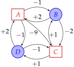
An ω-regular game (Γ,Win) is made of an arena Γ plus a winning
condi-tion Win. An arena is a tuple Γ= (V,E,hV0,V1i) where GΓ ,(V,E) is a
fi-nite directed graph and (V0,V1)is a partition of V into the set V0 of vertices
owned by Player 0 (a.k.a. Player ), and the set V1 of vertices owned by
Player 1 (a.k.a. Player #). A weighted arena is a tuple Γ= (V,E,w,hV0,V1i)
where: (V,E,hV0,V1i)is an arena, and GΓ,(V,E,w) is a finite weighted
di-rected graph. W.l.o.g. it can be assumed that GΓ has no sink, i.e., Nout(v) =
post(v)6=∅ for everyv∈V. Still, we remark thatGΓ is not required to be a bipartite graph on colour classes V0andV1. Fig. 1.3 depicts a simple example
of an arenaΓ.
A B
C D
−1
−2
+1
+2 − 1
−1
+1
+2
−9
Figure 1.3: An arenaΓ.
we find the pebble on some vertexvs∈V, which is called thestarting positionof
the game. At each turn, assuming the pebble is currently on a vertexv∈Vi (for i=0, 1), Playeri chooses an arc (v,v0)∈E and then the next turn starts with the pebble onv0. LetV+ andVω be the set of all finite and infinite sequences
on alphabetV, respectively. Givenπ∈Vω, let Inf(π)be the set of all and only
those verticesv∈Vthat appear infinitely often inπ; namely,
Inf(π),v∈V| ∀j∈N∃k∈Nsuch thatk>jandvk=v .
Generally, awinning condition is anyWin⊆Vω. The pair (Γ,Win,v
s)is called
agame, where it is given initial starting position vs∈V. A playis any infinite
pathπin Γ:
π,v0v1· · ·vn· · · ∈Vω.
The alphabet Ξ(π) of a play π is the set of all vertices v ∈V appearing in π at least once. Player 0 is declared the winner of the play π iff π ∈Win. Generally, it is interesting to considering those winning conditions that reflect the acceptance conditions in ω-automata [61]. We will not describe here the
theory ofω-automata, for which we refer the reader to the excellent reference
text [61], but we just recall the main – so called,ω-regular– winning conditions which can be defined for infinite games on graphs:
• M ¨uller condition: given a family of subsetsF ⊆2V, then:
WinF ,{π∈Vω|Inf(π)∈ F };
• Rabin condition: given a family F , {(E0,F0),(E1,F1), . . . ,(Em−1,Fm−1)},
whereEi,Fi⊆V for everyi, then:
WinF,{π∈Vω| ∃kInf(π)∩Ek =∅∧Inf(π)∩Fk 6=∅};
• Street condition: given a family F , {(E0,F0),(E1,F1), . . . ,(Em−1,Fm−1)},
whereEi,Fi⊆V for everyi, then:
WinF,{π∈Vω| ∀kInf(π)∩Ek 6=∅∨Inf(π)∩Fk=∅};
• Rabin chain condition: given a familyF,{(E0,F0),(E1,F1), . . . ,(Em−1,Fm−1)},
where Ei,Fi ⊆V for every i, and E0(F0(E1(F1(· · ·(Em−1(Fm−1,
then: it goes like the Rabin condition;
• Parity conditions: given a coloring function c:V →N on the vertices, then:
min-parity condition: Winc,{π∈Vω|min(Inf(π))is even};
• B ¨uchi condition: givenF ⊆V, then:
WinF ,{π∈Vω|Inf(π)∩ F 6=∅};
As argued in [61], the winning conditions can be transformed into one another, the transformations being exponential in the size of the transformed arenas. Under this prospect, the main result says that it is enough to consider theparity games (see Chapter 2, Subsection 2.4.2, Theorem 2.7 in [61]).
Concerning automata theory, let us just mention that the M ¨uller condi-tion plays a special role also in the theory ofω-automata, which are (roughly
speaking) finite-state automata takingω-words as input (see [61] for more
de-tails). The usual definitions of deterministic and nondeterministic automata are adapted to the case ofω-input-words by introducing new acceptance –
so-called, ω-regular acceptance – conditions. For this purpose one introduces an
acceptance componentin the specification of the automaton, which may arise in different formats. The acceptance component can be given as a set of states, as a family of sets of states, or as a function from the set of states to a fi-nite set of natural numbers. Indeed, for every ω-regular winning condition
as defined above there is a correspondingω-regularacceptance conditionwhich
leads to specific families of acceptance components. Then one may consider B ¨uchi, M ¨uller, Rabin, Street and Parity ω-automata. A remarkable result of McNaughtonandM ¨ullerasserts:
Theorem 1.6(Determinization of nondeterministic B ¨uchiω-automata [61, 84]).
Every nondeterministic B ¨uchi automaton with n states can be transformed into an equivalent (i.e., one accepting the sameω-language) deterministic M ¨uller automaton with2O(nlogn)states.
Let us proceed by discussing the determinacy properties ofω-regular games.
To this end, we recall next the notions offorgetfulandmemorylessstrategy.
Definition 1.21. For any i∈ {0, 1}, astrategyof Player i is any function,
σi:V∗×Vi→V,
such that for every finite path p0v in GΓ, where p0 ∈ V∗ and v∈ Vi, it holds that
(v,σi(p0,v))∈E. A play v0v1. . .vn. . .isconsistentwith a strategyσ∈Σi if vj+1= σ(v0v1. . .vj)whenever vj∈Vi. A strategy σi ∈Σi is said to befinite memory(or
forgetful) if there exists a finite set M, an element mI∈ M, and two functions,
δ:V×M→M and g:V×M→V,
such that the following holds. When p =v0v1· · ·vl−1 is a prefix of a play which is consistent withσi and the sequence m0,m1, . . . ,ml is determined by m0,mI and mi+1,δ(vi,mi), then it holds that:
A strategy σi of Player i is positional (or memoryless) if it doesn’t need any memory at all; namely, if it is forgetful for some singleton M, one such that|M|=1. The set of all the positional (memoryless) strategies of Player i is denoted byΣM
i .
Definition 1.22. Given a starting position vs∈V, theoutcomeof strategiesσ0∈Σ0
andσ1∈Σ1, denotedoutcomeΓ(vs,σ0,σ1), is the unique play that starts at vsand is consistent with both strategiesσ0∈Σ0andσ1∈Σ1.
Definition 1.23. Given a memoryless strategy σi∈ΣiM of Player i inΓ, then GσΓi =
(V,Eσi,w)is the graph obtained from GΓ by removing all arcs(v,v
0)∈E such that
v∈Vi and v06=σi(v); we say that GσΓi is obtained from G
Γby projectionw.r.t.σ
i.
A B
C D
−2
+2 −
1
−1
+1
+2
−9
Figure 1.4: An arena obtained by projection.
There are several questions to ask when one is confronted with aω-regular
game as introduced above.
• One may ask whether the game is determined, i.e., whether or not one of the players can move so that, regardless of how the other moves, the outcome play will always be winning for him. In that case, one can consider winning strategies and winning regions W0 and W1; where Wi
is the subset of verticesv∈V such that the Player i wins the game that starts atvs=v;
• One may ask whether it is possible to effectively (and maybe efficiently) compute which of the two players wins the game by starting from a given positionvs∈V;
• It is not only interesting to know who wins a game, but also how a winning strategy looks like, i.e., one may ask to automatically synthesize a winning strategy for the winning player.
It can be proved that, in every ω-regular game, both players win
forget-ful. This is called“forgetful (or finite memory) determinacy”of ω-regular games
(for a full proof see Chapter 2, Subsection 2.4.2, Corollary 2.15 in [61]). It is also worth mentioning that in every Rabin game, Player 0 has a memoryless winning strategy on his winning region. Symmetrically, in every Streett game, Player 1 has a memoryless strategy on his winning region (this is Theorem 2.16 in Chapter 2, Subsection 2.4.2, in [61]).
Theorem 1.7 (Determinacy of Parity Games [50, 122]). Parity Games, as well as all of the other ω-regular games, lie at the third level of the Borel Hierarchy, i.e.,
∆0
3=Σ03∩Π03. Hence, they are all determined by the Borel Determinacy Theorem. Particularly,Parity Gamesare memoryless determined.
Proofs of memoryless determinacy of parity games can be found e.g., in [50, 122]. The determinacy and the memorylessness of parity games is exploited in various areas. The word and emptiness problem for alternating tree automata as well as model-checking in modalµ-calculus can be reduced to deciding the
winner of a parity game. In fact, model checking µ-calculus is equivalent via
linear time reduction to determining parity games (for a proof see [50, 53, 61, 118]). Also, parity games offers an elegant tool to simplify Rabin’s proof of the decidability of the monadic second-order theory of the binary infinite tree (see e.g., [16, 50, 99]). In summary, the following result holds.
Theorem 1.8 ([50, 53, 61, 118]). The model-checking problem of modalµ-calculus is
linear-time equivalent to the problem of deciding if Player0 has a winning strategy from a given starting position in a given parity game; the game constructed from a transition system of size m and a formula of size n has size O(mn). Conversely, from a given parity game one can construct an equivalent transition system and a formula; the transition system is of the same size as the parity game.
1.4.3 From model-checking of Lµ to parity games
Let us provide a sketch of the construction from model-checking of modal
µ-calculus to determination of winning regions in parity games. Given a
sen-tence α of the modal µ-calculus, and a state s ∈S of a given transition
sys-tem M = S,{Ra}a∈A,{Pi}i∈N, the model-checking problem asks to decide whether α holds in s, i.e., M,s |=α. We aim at constructing a parity game G(M,α)in which Player 0 admits a winning strategy from a starting position
corresponding tosiff M,s|=α. Actually,G(M,α)is needed also for formulas α with free variables, so valuationsV are also taken into account. So we are
going to define a parity game GV(M,α), where GV(M,α) =G(M,α) when α is a sentence. To outline this construction, given a formula α, let us
con-sider theclosurecl(α)ofα, i.e., the smallest set containingαand closed under
subformulas and unfolding.
The game is defined as follows:
GV(M,α),
VGV(M,α),AGV(M,α),pGV(M,α),hV0GV(M,α),V1GV(M,α)i
,
where the vertex set is:
VGV(M,α),
n
(s,β)|sis a state ofM andβ∈cl(α) o
moreover, concerningV0GV(M,α) andV1GV(M,α):
(s,p)|s∈S\P} ∪
(s,¬p)|s∈S∩P} ⊆V0GV(M,α)
(s,p)|s∈S∩P} ∪
(s,¬p)|s∈S\P} ⊆V1GV(M,α)
where the intended interpretation is that (s,p)∈S× P will be declared win-ning for Player 0 (i.e., it will be a sink for Player 1) iff M,s |= p, i.e., s∈ P; otherwise, it will be winning for Player 1 and thus a sink vertex for Player 0. Symmetrically for(s,¬p). Similarly, concerning variables, one prescribes that:
(s,X)|s∈S\ V(X)} ⊆V0GV(M,α),
(s,X)|s∈S∩ V(X)} ⊆V1GV(M,α);
so that (s,X)∈S×Var will be declared winning for Player 0 (i.e., a sink for Player 1) iffM,s|=X, i.e.,s∈ V(X); otherwise, it will be winning for Player 1 and thus a sink vertex for Player 0.
Also, for everys∈Sand formulasα,β:
(s,α∨β)∈V0GV(M,α),
(s,α∧β)∈V1GV(M,α).
Finally, for everys∈S, for every a∈ Aand formulaβ:
(s,haiβ)∈V0GV(M,α),
(s,[a]β)∈V1GV(M,α).
Concerning positions such as(s,σX.β(X)), since they will have exactly one
outgoing arc in AGV(M,α) (see below), they can be controlled by anyone of the
two players. The arc setAGV(M,α)is defined by induction on the structure ofα:
• every position(s,p),(s,¬p)fors∈Sandp∈ P is a sink, i.e.,Nout(s,p) =
Nout(s,¬p) =∅for everys∈Sand p∈ P;
• similarly, every position(s,X)fors∈S andX∈Varis a sink;
• from positions(s,α∧β),(s,α∨β)there’s one arc to(s,α)and one to(s,β);
• from positions(s,haiβ),(s,[a]β)there’s one to (t,β)whenever(s,t)∈Ra;
• fixσ∈ {µ,ν}, from position(s,σX.β(X))there’s one to (s,β(σX.β(X))).
The priorities, pGV(M,α) :VGV(M,α)→N, are assigned as follows. Here the
interesting formulas are the fixpoint formulas σX.β(X), the µ formulas will
have odd priority and the ν formulas will have it even. All of the others
For anys∈Sand any subformula βofα:
pGV(M,α)(s,β),
2· badepth2 (X)c ifβis of the formνX.γ(X);
2· badepth2 (X)c+1 ifβis of the formµX.γ(X);
0 otherwise.
Notice that the alternation depth ofXis considered, not that ofβ, as this allows
one to assert a monotonicity property that is crucial for proving correctness of the construction (see [13] for the proof). To determine the winner of the game, themax-parity condition is adopted where the highest priority wins.
This concludes the description ofGV(M,α). Whenαis a sentence, it is fine
to denoteGV(M,α) =G(M,α). At this point, the following holds.
Theorem 1.9([13, 50]). For every sentenceαof the modalµ-calculus, for every
tran-sition systemM= S,{Ra}a∈A,{Pi}i∈N, and for every state s∈S:
M,s|=α ⇐⇒ Player 0 has a winning strategy starting from(s,α)inG(M,α).
The problem of deciding the winner of a parity game belongs to the com-plexity classesNP∩co-NP. Marcin Jurdz´ınski[70] proved a tighterUP∩co-UP
complexity bound and developed more efficient algorithms.
Definition 1.24. UP is the complexity class of decision problems solvable in
poly-nomial time on a unambiguousnon-deterministic Turing Machine; namely, one in which there is at most one accepting path for each input. Moreover, co-UP is the complexity class of decision problems whose complement lies inUP.
In summary, the following result holds.
Theorem 1.10 (Complexity of model-checking [52, 54, 70]). The model-checking
problem of the modalµ-calculus lies inNP∩co-NP; particularly, it lies inUP∩co-UP.
1.4.4 Mean-payoff games
In turn, the problem of determining parity games turns out to be reducible in polynomial-time to that of determining another family of infinite games on graphs, which is now recalled.
Definition 1.25 (Mean Payoff Games). A Mean Payoff Game (MPG) [14, 49,
123] is a game played on some arenaΓfor infinitely many rounds by two opponents, Player 0 gains a payoff defined as the long-run average weight of the play, whereas Player1loses that value. Formally, the Player0’spayoff of a play v0v1. . .vn. . .inΓ is defined as follows:
MP0(v0v1. . .vn. . .),lim inf n→∞
1
n n−1
∑
i=0
w(vi,vi+1).
The valuesecuredby a strategyσ0∈Σ0in a vertex v∈V is defined as:
valσ0(v), inf
σ1∈Σ1
MP0 outcomeΓ(v,σ0,σ1)
Notice that payoffs and secured values can be defined symmetrically for the Player 1
(i.e., by interchanging the symbol0with1andinfwithsup).
EhrenfeuchtandMycielski[49] proved that each vertexv∈Vadmits a unique
value, denoted valΓ(v), which each player can secure by means of a memory-less(orpositional) strategy. Moreover, uniformpositional optimal strategies do exist for both players, in the sense that for each player there exist at least one positional strategy which can be used to secure all the optimal values, inde-pendently with respect to the starting positionvs. Thus, for every MPGΓ:
∃σ
0∈Σ0M ∀v∈V
valσ0(v)≥valΓ(v)
,
and,
∃σ
1∈Σ1M ∀v∈V
valσ1(v)≤valΓ(v)
.
Indeed, the(optimal) valueof a vertexv∈Vin the MPGΓ is given [49, 123] by:
valΓ(v) = sup
σ0∈Σ0
valσ0(v) = inf
σ1∈Σ1
valσ1(v).
Definition 1.26(Optimal and Winning Strategies in MPGs). A strategyσ0∈Σ0
is optimal iff valσ0(v) =valΓ(v) for all v∈V. A strategy σ
0 ∈Σ0 is said to be winning for Player 0 iffvalσ0(v)≥0, and σ
1∈Σ1 is winning for Player 1 iff
valσ1(v)<0. Correspondingly, a vertex v∈V is a winning starting position for
Player0iffvalΓ(v)≥0; otherwise it is winning for Player1.
1.4.5 From parity games to mean-payoff games
We are now in the position to recall the reduction from parity games to MPGs.
Theorem 1.11(Reduction from Parity Games to Mean Payoff Games [70]). The
problem of deciding the winner in a Parity Game reduces in polynomial-time to the problem of deciding the winner in a Mean-Payoff Game.
Basically, in such reduction, given a parity gameΓ= (V,A,p,hV0,V1i)with
coloring/priority function p:V→N, one constructs an MPG with the same graph asΓand where all arcs are weighted with the following weight function (see [70]):
w(a),(−|V|)p(u), for every arca= (u,v)∈A.