DEPARTMENT OF INFORMATION ENGINEERING AND COMPUTER SCIENCE
ICT International Doctoral School
Efficient and Effective Solutions
for Video Classification
Ionut Cosmin Duta
Advisor:
Prof. Nicu Sebe University of Trento
Co-Advisor:
Prof. Bogdan Ionescu
University Politehnica of Bucharest
Contents
1 Introduction 3
2 Video classification with densely extracted HOG/HOF/MBH
features: an evaluation of the accuracy/computational
ef-ficiency trade-off 9
2.1 Introduction . . . 10
2.2 Related work . . . 12
2.3 Bag-of-Words for video . . . 14
2.3.1 Descriptor extraction . . . 14
2.3.2 Visual word assignment . . . 19
2.3.3 Classification . . . 21
2.4 Experiments . . . 21
2.4.1 Dataset . . . 22
2.4.2 Visual word assignment . . . 23
2.4.3 Comparison with Laptev et al. . . 25
2.4.4 Subsampling video frames . . . 28
2.4.5 Choice of Optical Flow . . . 32
2.4.6 Recommendations for practitioners . . . 36
2.4.7 Comparison to state-of-the-art . . . 37
3 Efficient Human Action Recognition using Histograms of
Motion Gradients and VLAD with Descriptor Shape
Infor-mation 41
3.1 Introduction . . . 42
3.2 Related work . . . 46
3.3 Proposed HMG method for descriptor extraction . . . 50
3.3.1 Histograms of Motion Gradients (HMG) . . . 50
3.3.2 Speed-up HMG extraction . . . 52
3.4 Proposed SD-VLAD method for descriptor encoding . . . . 54
3.4.1 VLAD representation . . . 55
3.4.2 Shape Difference for VLAD . . . 55
3.5 Experimental Evaluation . . . 59
3.5.1 Datasets . . . 59
3.5.2 Experimental setup . . . 60
3.5.3 Comparison to dense descriptors . . . 61
3.5.4 Feature Encoding . . . 63
3.5.5 Comparison with Improved Dense Trajectories . . . 72
3.5.6 Frame subsampling . . . 73
3.5.7 Real-time video classification . . . 76
3.5.8 Comparison to state-of-the-art . . . 78
3.6 Conclusion . . . 80
4 Spatio-Temporal Vector of Locally Max Pooled Features for Action Recognition in Videos 81 4.1 Introduction . . . 82
4.2 Related work . . . 86
4.3 Proposed ST-VLMPF encoding method . . . 87
4.4 Local deep features extraction . . . 91
4.5.1 Datasets . . . 94
4.5.2 Experimental setup . . . 95
4.5.3 Parameter tuning . . . 96
4.5.4 Comparison to other encoding approaches . . . 98
4.5.5 Fusion strategies . . . 100
4.5.6 Comparison to state-of-the-art . . . 102
4.6 Conclusion . . . 103
5 Conclusions and Future Work 105
PUBLICATIONS
This thesis consists of the following publications:
• Chapter 2:
Uijlings, J.R.R.; Duta, I.C.; Sangineto, E. and Sebe, N. ”Video classi-fication with Densely extracted HOG/HOF/MBH features: an evalu-ation of the accuracy/computevalu-ational efficiency trade-off”. In Interna-tional Journal of Multimedia Information Retrieval, 4(1):33-44, 2015. Idea previously appeared in:
Uijlings, J.R.R.; Duta, I.C.; Rostamzadeh, N. and Sebe, N. ”Real-time video classification using dense HOF/HOG”. In International Conference on Multimedia Retrieval (ICMR), 2014.
• Chapter 3:
Duta, I.C.; Uijlings, J.R.R.; Aizawa, K.; Hauptmann, A.G.; Ionescu, B. and Sebe, N. ”Efficient Human Action Recognition using His-tograms of Motion Gradients and VLAD with Descriptor Shape In-formation”. In Multimedia Tools and Applications (MTAP), DOI: 10.1007/s11042-017-4795-6, 2017.
Part of the idea previously appeared in:
Duta, I.C.; Uijlings, J.R.R.; Nguyen, T. A.; Aizawa, K.; Haupt-mann, A.G.; Ionescu, B. and Sebe, N. ”Histograms of Motion Gra-dients for Real-time Video Classification” In International Workshop on Content-based Multimedia Indexing (CBMI), 2016.
• Chapter 4:
The papers published during the course of the PhD but not included in this thesis are the following:
• Duta, I.C.; Ionescu, B.; Aizawa, K. and Sebe, N. ”Simple, Efficient and Effective Encodings of Local Deep Features for Video Action Recogni-tion”. In International Conference on Multimedia Retrieval (ICMR), 2017.
• Duta, I.C.; Ionescu, B.; Aizawa, K. and Sebe, N. ”Spatio-temporal VLAD Encoding for Human Action Recognition in Videos”. In Inter-national Conference on Multimedia Modeling (MMM), 2017.
• Duta, I.C.; Nguyen, T.A.; Aizawa, K.; Ionescu, B. and Sebe, N. ”Boosting VLAD with Double Assignment using Deep Features for Action Recognition in Videos”. In International Conference on Pat-tern Recognition (ICPR), 2016.
• Mironica, I.; Duta, I.C.; Ionescu, B. and Sebe, N. ”A modified vector of locally aggregated descriptors approach for fast video classifica-tion”. In Multimedia Tools and Applications (MTAP), 75(15):9045-9072, August 2016.
Chapter 1
Introduction
Video understanding is one of the long-standing goals of the computer vision and multimedia communities. The ability to automatically under-stand video content opens the door to a huge pool of potential applica-tions such as automatic video analysis, video indexing and retrieval, video surveillance, virtual reality, human-computer interaction, robot learning, etc. Video is one of the most notorious multimedia content for entertain-ment and communication. A statistical study1 reveals that on YouTube there are currently updated more than 300 hours of video every minute, each day YouTube users watch more than a billion hours of video. This explosive growth in video content continues to have a fulminant increase, for instance Cisco forecast2 mentioned that the IP video would account for 80% of all IP traffic by 2019. Given this fulminant growth in video content, the capability of computers to perform video classification becomes very challenging and crucial for various purposes such as search, recommenda-tion, ranking, etc.
Computers are far behind humans in understanding video content. Be-sides the enormous amount of video content, it is very challenging to per-form video classification due to many reasons such as large intra-class
varia-1
https://www.youtube.com/yt/about/press/
tions, viewpoint changes, background clutter, high dimension of video data, low video resolution, camera motion, etc. All of these make video classifi-cation a very challenging and computationally demanding task, however, video classification has received a sustained attention from the research community due to the unlimited potential of real-life applications.
The aim of this PhD thesis is to make a step forward towards teaching computers to understand videos in a similar way as humans do. In this work we tackle the video classification and/or action recognition tasks. This thesis was completed in a period of transition, the research commu-nity moving from traditional approaches (such as hand-crafted descriptor extraction) to deep learning. Therefore, this thesis captures this transition period, however, unlike image classification, where the state-of-the-art re-sults are dominated by deep learning approaches, for video classification the deep learning approaches are not so dominant. As a matter of fact, most of the current state-of-the-art results in video classification are based on a hybrid approach where the hand-crafted descriptors are combined with deep features to obtain the best performance. This is due to several factors, such as the fact that video is a more complex data as compared to an image, therefore, more difficult to model and also that the video datasets are not large enough to train deep models with effective results.
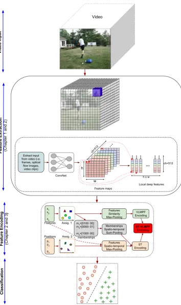
x1 x2 ⋮ xn p1 p2 ⋮ pn VLMPF Encoding ST Encoding ST-VLMPF Encoding m1=[0100⋯00]
m2=[0000⋯01]
⋮ mn=[1000⋯00]
memberships Features Positions Assig. 1 Assig. 2 Memberships Spatio-temporal Sum-Pooling Features Similarity Max-Pooling Features Spatio-temporal Max-Pooling Video ConvNet ch=512 ch=512 h w
h x w
Feature maps
Local deep features Extract input
from video (i.e. frames, optical flow images,
video clips)
Video Input
Feature Extraction (Chapter 1 and 2)
Feature Encoding (Chapter 2 and 3
)
Classification
This thesis is mainly based on three works. The first work focuses on descriptor extraction, which is an important step in the video classification pipeline. The second and the third works tackle the feature encoding part which is highly dependent on the descriptor extraction step. At the end, the feature encoding approach drastically influences the classifier performance. One of the bottlenecks of the video classification pipeline is represented by the feature extraction step, where most of the approaches are extremely computationally demanding, what makes them not suitable for real-time applications. In this thesis, we tackle this issue, propose different speed-ups to improve the computational cost and introduce a new descriptor that can capture motion information from a video without the need of computing optical flow (which is very expensive to compute). Another important component for video classification is represented by the feature encoding step, which builds the final video representation that serves as input to a classifier. During the PhD, we proposed several improvements over the standard approaches for feature encoding. We also propose a new feature encoding approach for deep feature encoding. To summarize, the main contributions of this thesis are as follows3:
• We propose several speed-ups for descriptor extraction, providing a version for the standard video descriptors that can run in real-time. We also investigate the trade-off between accuracy and computational efficiency.
• We provide a new descriptor for extracting information from a video, which is very efficient to compute, being able to extract motion infor-mation without the need of extracting the optical flow.
• We investigate different improvements over the standard encoding approaches for boosting the performance of the video classification
pipeline.
• We propose a new feature encoding approach specifically designed for encoding local deep features, providing a more robust video represen-tation.
The remainder of this thesis is organized as follows:
• In Chapter 2, we present our work on descriptor extraction for video classification, where we address one of its issues: high computational cost. Specifically, the contributions are: (1) We propose several speed-ups for densely sampled HOG (Histogram of Orientated Gradients), HOF (Histogram of Optical Flow) and MBH (Motion Boundary His-tograms) descriptors and release Matlab code; (2) We investigate the trade-off between accuracy and computational efficiency of descriptors in terms of frame sampling rate and type of Optical Flow method; (3) We investigate the trade-off between accuracy and computational efficiency for computing the feature vocabulary, using and compar-ing most of the commonly adopted vector quantization techniques: k-means, hierarchical k-means, Random Forests, Fisher Vectors and Vector of Locally Aggregated Descriptors (VLAD).
responses, reuse subregions of aggregated magnitude responses, and frame subsampling, which make the pipeline more efficient. (4) We propose an integration of our descriptor and encoding method in a specifically designed video classification framework which allows for real-time performance while maintaining the high accuracy of the re-sults.
• Chapter 4 continues the work on feature encoding. Specifically, the contributions are: (1) Provide a new encoding approach specifically designed for working with deep features. We exploit the nature of deep features, with the goal of capturing the highest feature responses from the highest neuron activation of the network. (2) Efficiently incorpo-rate the spatio-temporal information within the encoding method by taking into account the features position and specifically encode this aspect. Spatio-temporal information is crucially important when deal-ing with video classification. (3) Provide an action recognition scheme to work with deep features, which can be adopted to obtain impres-sive results with any already trained network, without the need for re-training or fine tuning on a particular dataset. Furthermore, our framework can easily combine different information extracted from dif-ferent networks. In fact, our pipeline for action recognition provides a reliable representation outperforming the previous state-of-the-art approaches, while maintaining a low complexity.
Chapter 2
Video classification with densely
extracted HOG/HOF/MBH
features: an evaluation of the
accuracy/computational efficiency
trade-off
1
A widely used framework in video classification is based on Bag-of-Words using local visual descriptors. Most commonly these are Histogram of Ori-ented Gradient (HOG), Histogram of Optical Flow (HOF) and Motion Boundary Histogram (MBH) descriptors. While such approach is very powerful for classification, it is also computationally expensive. This work addresses the problem of computational efficiency. Specifically: (1) We propose several speed-ups for densely sampled HOG, HOF and MBH de-scriptors and release Matlab code; (2) We investigate the trade-off between accuracy and computational efficiency of descriptors in terms of frame sam-pling rate and type of Optical Flow method; (3) We investigate the trade-off
1Uijlings, J.R.R.; Duta, I.C.; Sangineto, E. and Sebe, N. ”Video classification with Densely
extracted HOG/HOF/MBH features: an evaluation of the accuracy/computational efficiency
between accuracy and computational efficiency for computing the feature vocabulary, using and comparing most of the commonly adopted vector quantization techniques: k-means, hierarchical k-means, Random Forests, Fisher Vectors and VLAD.
2.1
Introduction
The Bag-of-Words method [14, 72] has been successfully adapted from the domain of still images to the domain of video by using local, visual, space-time descriptors (e.g. [46, 19, 41, 66, 67, 86]). Successful applications range from Human Action Recognition [46, 44, 63] to Event Detection [73] and Concept Classification [74, 73]. However, analyzing video is even more computationally expensive than analysing images. Hence, in order to deal with the enormous, growing amount of digitalized video it is important to have not only accurate, but also computationally efficient methods.
this evaluation chapter makes the following contributions:
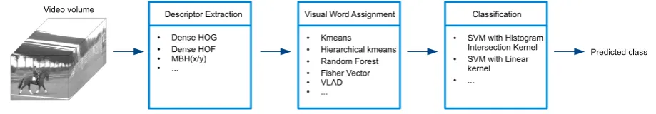
!"#$%&'#$(&)*++ ,#+&"%-'."(/0'"*&'%.1 2%+3*)(4."$(5++%617#1' 8)*++%9%&*'%.1
! ,#1+#(:;< ! ,#1+#(:;= ! >?:@0ABC ! DDD
! E7#*1+ ! :%#"*"&F%&*)(G7#*1+ ! H*1$.7(=."#+' ! =%+F#"(2#&'." ! 2I5, ! DDD
! J2>(K%'F(:%+'.6"*7 L1'#"+#&'%.1(E#"1#) ! J2>(K%'F(I%1#*"
G#"1#) ! DDD 2%$#.(M.)37#
Figure 2.1: General framework for video classification using a Bag-of-Words pipeline. The methods evaluated in this work are instantiated in this diagram.
Fast Dense HOG/HOF/MBH. We exploit the nature of densely
sampled descriptors in order to speed up their computation. HOG, HOF and MBH descriptors are created from subvolumes. These subvolumes can be shared by different descriptors similar to what was done in [83]. In this work we generalize their idea of reusing subregions to 3 dimensions. Matlab source code is available2.
Evaluation of frame subsampling. Videos consist of many frames,
making them computational expensive to analyze. However, subsequent frames also largely carry the same information. In this work we evaluate the trade-off between accuracy and computational efficiency when subsampling video frames.
Evaluation of Optical Flow. Calculating optical flow is generally
expensive and takes up much of the total HOF and MBH descriptor ex-traction time. But for optical flow there is also a trade-off between com-putational efficiency and accuracy. Moreover, optical flow methods are generally tested against optical flow benchmarks such as [3, 10], but it is not immediately obvious that methods which perform well on these bench-marks would automatically also yield better HOF and MBH descriptors.
Therefore in this work we evaluate optical flow methods directly in our task of interest: video classification. Specifically, we compare the opti-cal flow methods of Lukas-Kanade [49], Horn-Schunk [32], Farneb¨ack [28], Brox 04 [8], and Brox 11 [9].
Evaluation of descriptor encoding. The classical way of
transform-ing a set of local visual descriptors into a stransform-ingle fixed-length vector is by using a k-means visual vocabulary and assign local descriptors to the mean of the nearest cluster (e.g. [14]). However, both hierarchical k-means and Random Forests [53, 83] are viable fast alternatives. Furthermore, the Fisher Vector [61] significantly outperforms classical k-means representa-tion in many tasks, whereas VLAD [35] can be considered a simplified non-probabilistic version of the Fisher Vector [64] and it is computationally more efficient. In this work we evaluate the accuracy/efficiency trade-off of all five methods above in the context of video classification.
2.2
Related work
in this chapter we implemented and evaluated the descriptors which are most widely used: HOG, HOF and MBH.
Wang et al. [90] evaluated several interest point selection methods and several spatio-temporal descriptors. They found that dense sampling meth-ods generally outperform interest points, especially on more difficult datasets. As this result was earlier found in image analysis [37, 65], this work focuses on dense sampling for videos. In [90] the evaluation was on accuracy only. In contrast, this work focuses on the trade-off between computational effi-ciency and accuracy.
Wang et al. [86] proposed to use dense trajectories. In their method, the local video volume moves spatially through time; it tries to stay on the same part of the object. Additionally, they use changes in optical flow rather than the optical flow itself. They show good improvements over normal HOG, HOF and MBH descriptors. Nevertheless, combining their dense trajectory descriptors with both normal HOG, HOF and MBH descriptors still gives significant improvements over dense trajectories alone [39, 86]. In this work we focus on HOG, HOF and MBH. Note that we evaluate the accuracy/efficiency trade-off for several optical flow methods which may be of interest also when using dense trajectories.
The Fisher Vector [61] has been shown to outperform standard vector quantization methods such as k-means in the context of Bag-of-Words. On the other hand, the recently proposed VLAD descriptors [35] can be seen as a non-probabilistic version of Fisher Vectors which are faster to compute [35, 64]. In this work we evaluate the accuracy/efficiency trade-off using Fisher Vector and VLAD in the context of video classification.
2.3
Bag-of-Words for video
In this section we explain in detail the pipeline that we use. We mostly use off-the-shelf yet state-of-the-art components to construct our Bag-of-Words pipeline, which is necessary for a good evaluation. Additionally, we explain how to create a fast implementation of densely sampled HOG and HOF descriptors, and also implicitly for MBH, being MBH based on HOG and Optical Flow. We make the HOG/HOF/MBH descriptor code publicly available.
2.3.1 Descriptor extraction
Fast dense HOG/HOF descriptors
For both HOG and HOF descriptors, there are several steps. First one needs to calculate either gradient magnitude responses in horizontal and vertical directions (for HOG), or optical flow displacement vectors in hor-izontal and vertical directions (for HOF). Both result in a 2-dimensional vector field per frame. Then for each response the magnitude is quantized in o orientations, usually o = 8. Afterwards, one needs to aggregate these responses over blocks of pixels in both spatial and temporal directions. The next step is to concatenate responses of several adjacent pixel blocks. Fi-nally, descriptors have to be normalized and sometimes PCA is performed to reduce their dimensionality, often leading to computational benefits or improved accuracy.
To calculate gradient magnitude responses we use HAAR-features. These are faster to compute than Gaussian Derivatives and have proven to work better for HOG [15]. Quantization in o orientations is done by dividing each response magnitude linearly over two adjacent orientation bins.
We use the classical Horn-Schunk [32] method for optical flow responses as a default. We use the version implemented by the Matlab Computer Vision System Toolbox. Additionally, we evaluate four other optical flow methods: Lucas-Kanade [49], also using the Matlab Computer Vision Sys-tem Toolbox, the method of F¨arneback [28], using OpenCV3 with the mex-opencv interface4, Brox 04 [8], and Brox 11 [9] using the author’s publicly available code.
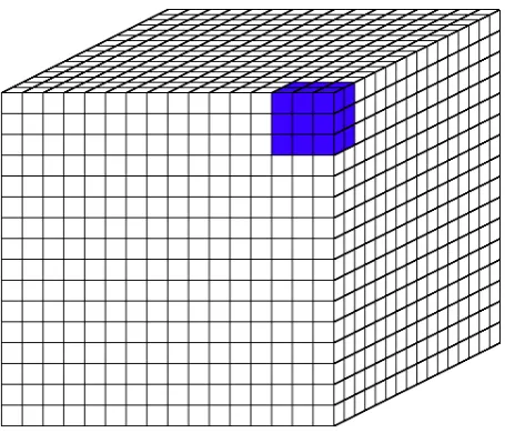
Both HOG and HOF descriptors are created out of blocks. By choosing the sampling rate identically to the size of a single block, one can reuse these blocks. Figure 2.2 shows an example on how a video volume can be divided into blocks. Once responses per block are computed, descriptors
3http://opencv.org
Figure 2.2: Blocks in a video volume can be reused for descriptor extraction. In our work descriptors consist of 3 by 3 blocks in space and 2 blocks in time, shown in blue.
can be formed by concatenating adjacent blocks. In this work we use descriptors of 3 by 3 blocks in the spatial domain and 2 blocks in the temporal domain, as shown in blue in Figure 2.2, but these parameters can be easily changed. Hence each block is reused 18 times (except for the blocks on the borders of the video volume).
To aggregate responses over space we use the Matlab-friendly method proposed by [83]: Let R be an N × M matrix containing responses in a single orientation (be it gradient magnitude or optical flow magniture). Let BN and BM be the number of elementary blocks from which HOG/HOF
features are composed. Now it is possible to construct (sparse) matrices O and P of respectively BN ×N and M ×BM such that ORP = A, where A
is a BN ×BM matrix containing the aggregated responses for each block.
single block. For more details we refer the reader to the work of [83]. In this work, we extract descriptors on a single scale where blocks consist of 8 by 8 pixels by 6 frames, which at the same time is our dense sampling rate. Descriptors consist of 3 by 3 by 2 blocks. Both for HOG and HOF the magnitude responses are divided into 8 orientations, resulting in 144 dimensional descriptors. PCA is performed to reduce the dimensionality by 50% resulting in 72 dimensional vectors. Afterwards, normalization is performed by the L1-norm followed by the square root, which effectively means that Euclidean distances between descriptors in fact reflect the often superior Hellinger distance [1].
Motion Boundary Histograms descriptor
Another commonly used descriptor for video classification tasks is Motion Boundary Histogram (MBH), proposed by Dalal et al. [16], who proved its robustness to camera and background motion. The intuitive idea of MBH is to represent the oriented gradients computed over the vertical and the horizontal optical flow components. The advantage of such representation is that constant camera movements tend to disappear and the description focuses on optical flow differences between frames (motions boundaries).
In more detail, the optical flow’s horizontal and vertical components are separately represented using two scalar maps, which can be seen as gray-level “images” of the motion components. Histograms of oriented gradients are then computed for each of the two optical flow component images, using the same approach used for computing HOG in still images. Taken into account only flow differences, the information about changes in motion boundaries is kept and the constant motion information is removed, which leads to the cancelation of most of the effects of camera motion.
components, histograms of oriented gradients are computed on each image component using the same efficient approach and the same parameters shown in Section 2.3.1. Also the block-based aggregation step is analogous to what described in Section 2.3.1.
The outcome of this process is a pair of horizontal (MBHx) and vertical (MBHy) descriptors [16], each one composed of 144 dimensions. We sep-arately apply PCA to both MBHx and MBHy and we obtain two vectors of 72 dimensions each. The (PCA-reduced) MBHx and MBHy vectors can then be either separately used in the subsequent visual word assignment and classification stages (Figure 2.1) or combined in order to get a unique descriptor. In [86] the authors state that late fusion of MBHx and MBHy gives a better performance than concatenating the two descriptors before the visual word assignment step. Hence in this work we will report results for MBHx and MBHy separately, and a late fusion of the two which we simply denote as MBH. This late fusion combines the outcomes of the two (independent) classifications with equal weights. Finally, in Section 2.4.6, we will also show results concerning a late fusion strategy involving all the descriptors (MBHx, MBHy, HOG and HOF).
Existing HOG/HOF descriptors
We use the existing implementation of Laptev et al. [46]. We use the default parameters as suggested by the authors, which compared to our descriptors are as follows: They perform a dense sampling at multiple scales. At the finest scale, blocks are 12 by 12 pixels by 6 frames, sampling rate is every 16 pixels by every 6 frames. They consider 8 spatial scales and 2 temporal scales for a total of 16 scales, where each scale increases the descriptor size by a factor of √2. In the end, they generate around 33% less descriptors than our single scale dense sampling method.
ori-entations for HOG and 5 oriori-entations for HOF, resulting in respectively 72 and 90 dimensional descriptors.
2.3.2 Visual word assignment
We use five different ways of creating a single feature representation of a set of descriptors extracted from a single video: k-means, hierarchical k-means, Random Forests [7, 31], VLAD [35] and Fisher Vectors [61].
For hierarchical k-means we use the implementation made available by VLFeat [84]. For the regular k-means assignment, we make use of the fact that the descriptors are L2-normalised: Euclidean distances are pro-portional to dot products (cosine of angles) between the vectors. Hence finding the minimal euclidean distance is equivalent to finding the maxi-mal dot product, yet more efficient to compute [83]. For both hierarchical k-means and regular k-means, we use 4096 visual words. For hierarchical k-means, we learn a hierarchical tree of depth 2 with 64 branches per node of the tree (preliminary experiments showed a large decrease in accuracy when using a higher depth with fewer branches, but only marginal im-provements in computational efficiency, data not shown). We normalize the resulting frequency histograms using the square root, which discounts frequently occurring visual words, followed by L1-normalization.
Random Forests are binary decision trees which are learned in a super-vised way by randomly picking several descriptor dimensions at each node with several random thresholds and choose the one with the highest En-tropy Gain. We follow the recommendations of [83], using 4 binary decision trees of depth 10, resulting in 4096 visual words. The resulting vector is normalized by taking the square root followed by L1.
descrip-tors is represented as the gradient with respect to the parameters of the GMM. This can be intuitively explained in terms of the EM algorithm for GMMs: Let Gλ be the learned GMM with parameters λ. Now use the
E-step to assign the set of descriptors D to Gλ. Then the M-step yields
a vector F with adjustments on how λ should be updated to fit the data (i.e. how the GMM clusters should be adjusted). This vector F is exactly the Fisher Vector representation. We follow [61] and normalize the vector using a square root of the absolute values and afterwards keep the original sign ((sign(fi))
p
|fi|), followed by L2. In this work we use two common
cluster sizes for the GMM: 64 and 256 clusters [61]. Without a spatial pyra-mid [47], for our 72 dimensional HOG/HOF/MBHx/MBHy features this will yield vectors of 9,216 and 36,864 dimensions respectively. While not comparable with the dimensionality of other methods, Fisher Vectors (and VLAD) allow for linear Support Vector Machines rather than Histogram Intersection or χ2-kernels. Hence efficiency-wise, the simpler classifiers will compensate for the larger dimension of the feature vectors.
The recently proposed VLAD [35] representation can be seen as a sim-plification of the Fisher Vector [35, 64] in which: (1) a spherical GMM is used, (2) the soft assignment is replaced with a hard assignment and (3) only the gradient of Gλ with respect to the mean is considered (first
order statistics). This leads to a lower dimensional representation, half of the dimensions of a Fisher Vector, in which second order statistics are also used. Following [35] we use for VLAD the same normalization scheme used for Fisher Vectors: We square-root the VLAD vectors while keeping their sign, followed by L2-normalisation. For good comparison to the Fisher Vectors, we use a dictionary of 128 and 512 clusters respectively, leading to features of dimensionality identical to the Fisher Vectors: 9,216 and 36,864 dimensions.
divide each video volume into the whole video and into three horizontal parts which intuitively roughly corresponds to a ground, object, and sky division (in outdoor scenes).
2.3.3 Classification
For classification we use Support Vector Machines which are powerful and widely used in a Bag-of-Words context (e.g. [14, 47, 83, 84]). For k-means, hierarchical k-means, and Random Forests, we use SVMs with the His-togram Intersection kernel, using the fast classification method as proposed by [50]. For the Fisher Vector and VLAD, we use linear SVMs. For both types of SVMs, we make use of the publicly available LIBSVM library [11] and the fast Histogram Intersection classification of [50].
2.4
Experiments
Our baseline consists of densely sampled HOG, HOF and MBH(x/y) de-scriptors, all consisting of blocks of 8 by 8 pixels by 6 frames. For HOF and MBH(x/y), optical flow is calculated using Horn-Schunk. Gradient and flow magnitude responses are quantized in 8 bins. The final descrip-tors consist of 3 by 3 by 2 blocks. PCA always reduces dimensionality of descriptors by 50%. We use a spatial pyramid division of 1 ×1× 1 and 1×3× 1 [47] (we have no temporal division). Normalisation after word assignment is done by either taking the square root while keeping the sign followed by L2 for the Fisher Kernel, or by the square root plus L1 for all other methods. We use SVMs for classification, with either a linear kernel for the Fisher Vectors or histogram intersection kernel for all other visual word assignment methods.
k-means, Random Forests, VLAD and the Fisher Kernel; (2) We compare our densely extracted descriptors with the descriptors provided by Laptev et al. [46]; (3) We evaluate the efficiency/accuracy trade-off by subsam-pling video frames for the descriptor extraction process; (4) For HOF and MBH(x/y) descriptors, we compare five different optical flow implementa-tions: Horn-Schunk, Lukas-Kanade, Farneb¨ack [28], Brox 04 [8] and Brox 11 [9].
All timing experiments are performed on a single core of an Intel(R) Xeon(R) CPU E5620 2.40GHz. We use mainly Matlab, but most tool-boxes used by us have mex-interfaces to c++ implementations for critical functions. All implementations are heavily optimized for speed. Since the computation involves many common operations that use standardized and optimized libraries (e.g. convolutions, matrix multiplications) on large quantities of data, virtually the entire time is spent on core calculations while the overhead is negligible; using only c++ will not result in noticeable differences in the overall timing results presented in this work.
Based on our experiments we provide two recommendations, one for real-time video classification and one for accurate video classification. Fi-nally we give a comparison with the state-of-the-art.
2.4.1 Dataset
standard procedure we perform a leave-one-group-out cross-validation and report the average classification accuracy over all 25 folds. Optimization of the SVM slack parameter is done for every class for every fold on the training set (containing 24 groups).
2.4.2 Visual word assignment
In this experiment we compare the following visual word assignment meth-ods: k-means, hierarchical k-means, Random Forests, VLAD and Fisher Vector. K-means, hierarchical k-means and Random Forests are similar in the sense that the final vector represents visual word counts. To com-pare these methods we ensure that all have 4096 visual words. For k-means this k-means performing clustering with k=4096. For hierarchical k-means we use a hierarchy of depth 2 with 64 branches at each node. The Random Forest consists of 4 trees of depth 10. We choose to base our Fisher Vectors on standard sizes for the number of clusters: 64 and 256 clusters [61, 12]. While Fisher Vectors are of higher dimensionality, the vectors work with linear classifiers. This means that Fisher Vectors are best compared with the other visual word assignment methods in terms of the accuracy/efficiency trade-off. Similarly, we adopted 2 standard clus-ter sizes for VLAD: 128 and 512 dimensions respectively [35] and we used linear classifiers as well.
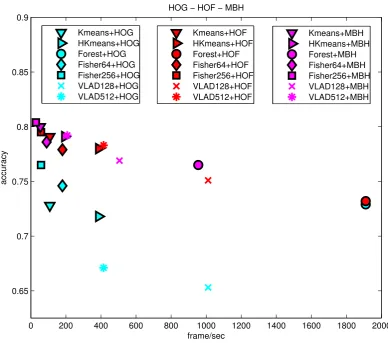
0 200 400 600 800 1000 1200 1400 1600 1800 2000 0.65
0.7 0.75 0.8 0.85 0.9
HOG − HOF − MBH
frame/sec
accuracy
Kmeans+HOG HKmeans+HOG Forest+HOG Fisher64+HOG Fisher256+HOG VLAD128+HOG VLAD512+HOG
Kmeans+HOF HKmeans+HOF Forest+HOF Fisher64+HOF Fisher256+HOF VLAD128+HOF VLAD512+HOF
Kmeans+MBH HKmeans+MBH Forest+MBH Fisher64+MBH Fisher256+MBH VLAD128+MBH VLAD512+MBH
Figure 2.3: Accuracy/Efficiency trade-off for various word assignment methods and fea-tures. For a better readability of the figure, we omitted the results concerning MBHx and MBHy (see Table 3.2).
k-means hk-means RF FV 64 FV 256 VLAD 128 VLAD 512 HOG Acc 0.728 0.718 0.729 0.746 0.765 0.653 0.671 HOF Acc 0.791 0.780 0.732 0.779 0.795 0.751 0.783 MBHx Acc 0.782 0.774 0.738 0.767 0.796 0.749 0.774 MBHy Acc 0.772 0.763 0.739 0.759 0.787 0.737 0.765 MBH Acc 0.800 0.791 0.765 0.786 0.804 0.769 0.792 sec/video 1.81 0.51 0.10 1.10 3.39 0.19 0.47
frame/sec 108 387 1910 180 58 1011 415
Table 2.1: Trade-off accuracy/efficiency for the following visual word assignment methods: k-means, hierarchical k-means (hk-means), Random Forest (RF), Fisher Kernel with 64 and 256 clusters (FK 64 and FK 256). Assignment time for HOG and HOF is the same. In terms of classification time per video, we measure 0.017 seconds per video when using the fast Histogram Intersection based classification for SVMs [50] for k-means, hk-means, and Random Forests. We measure 0.001 seconds per video for the linear classifier used on the Fisher Vector representation with 256 clusters. This means that the classification time is negligible compared to the word assignment time and is of little concern for video classification.
For the remainder of this work, we choose to perform our evaluation on two word assignment methods: the Fisher Vector, which yields the most accurate results, and hk-means, which is the second fastest after Random Forests, while its accuracy for HOF and MBH(x/y) is much higher than using Random Forests.
2.4.3 Comparison with Laptev et al.
com-0 0.1 0.2 0.3 0.4 0.5 0.6 0.7 0.8 0.9 1 HOF+Fisher
HOF+HKmeans HOG+Fisher HOG+HKmeans
accuracy Laptev et al.
Ours
Figure 2.4: Accuracy comparison between [46] and our HOG/HOF descriptors parison because the code in [46] does not include any implementation for MBH features. Results are presented in Figures 2.4 and 2.5 and in Ta-ble 2.2.
hk-means FV 256 efficiency HOG HOF HOG HOF sec/vid frame/sec [46] 0.657 0.590 0.670 0.725 141 1.4 ours 0.718 0.780 0.765 0.795 15 12.8
Table 2.2: Comparing the dense HOG/HOF implementation of [46] and ours. The de-scriptor extraction time is measured for extracting both HOG and HOF features, as the binary provided by [46] does always both. Descriptor extraction time is independent of the visual word assignment method (RF or FV 256).
0 2 4 6 8 10 12 14 16 Laptev et al.
Ours
frame/sec
Figure 2.5: Computational Efficiency comparison between [46] and our HOG/HOF de-scriptors
for [46] and 0.795 accuracy for our implementation. These are accuracy increases of 9% and 7% respectively. Similar differences are obtained using hk-means. Part of the difference can be explained by the fact that we sam-ple differently: because we reuse blocks of the descriptors, our sampling rate is defined by the size of a single block. This means we sample descrip-tors every 8 pixels and every 6 frames at a single scale, whereas [46] samples every 16 pixels and every 6 frames at 10 increasingly course scales. For our method this yields around 150 descriptors per frame or around 29,000 de-scriptors per video whereas [46] generates around 90 dede-scriptors per frame or around 17,500 descriptors per video, which means we generate 66% more descriptors. While this may seem unfair towards [46], in this work we are interested in the trade-off between accuracy and computational efficiency, which makes the exact locations from where descriptors are sampled irrel-evant.
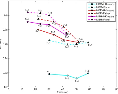
0 10 20 30 40 50 60 70 80 0.7 0.72 0.74 0.76 0.78 0.8 F=1 F=2 F=3 F=6 F=1
F=2 F=3 F=6
F=1 F=2 F=3 F=6 F=1 F=2 F=3 F=6 F=1 F=2 F=3 F=6 F=1 F=2 F=3 F=6 frame/sec accuracy HOG+HKmeans HOG+Fisher HOF+HKmeans HOF+Fisher MBH+HKmeans MBH+Fisher
Figure 2.6: Trade-off accuracy/efficiency when varying sampling rate. F stands for frames per block and it is directly related to sampling rate.
To conclude, our implementation is significantly faster and significantly more accurate than the version of [46].
2.4.4 Subsampling video frames
In video, subsequent video frames largely contain the same information. As the time for descriptor extraction is the largest bottleneck in video classification, we investigate how the accuracy behaves if we subsample video frames and hence speed-up the descriptor extraction process.
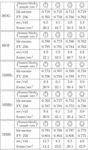
HOG frames/block sample rate 6 1 3 2 2 3 1 6
hk-means 0.718 0.716 0.712 0.719 FV 256 0.765 0.759 0.760 0.762 sec/vid 6.5 4.5 3.9 3.3 frame/sec† 30.2 43.7 50.3 58.9
HOF frames/block sample rate 6 1 3 2 2 3 1 6
hk-means 0.780 0.773 0.766 0.762 FV 256 0.795 0.791 0.784 0.763 sec/vid 8.9 5.9 4.8 3.8 frame/sec† 22.1 33.5 40.7 51.8
MBHx frames/block sample rate 6 1 3 2 2 3 1 6
hk-means 0.774 0.767 0.769 0.758 FV 256 0.796 0.794 0.788 0.771 sec/vid 9.4 6.1 5.0 3.9 frame/sec† 20.9 32.1 39.4 50.7
MBHy frames/block sample rate 6 1 3 2 2 3 1 6
hk-means 0.763 0.757 0.752 0.741 FV 256 0.787 0.785 0.772 0.750 sec/vid 9.4 6.1 5.0 3.9 frame/sec† 20.9 32.1 39.4 50.7
MBH frames/block sample rate 6 1 3 2 2 3 1 6
hk-means 0.791 0.788 0.787 0.772 FV 256 0.804 0.803 0.800 0.775 sec/vid 13.7 8.3 6.5 4.6 frame/sec† 14.3 23.6 30.1 42.9
pixels by 6 frames. To subsample in such a way that every block describes the same video volume regardless of the sampling rate, we do the following: if we sample every 2 frames, we aggregate responses over 3 frames (i.e. of frame 2, 4 and 6). When sampling every 3 frames, we aggregate responses over 2 frames (i.e. frame 2 and 5), and when sampling every 6 frames in which we only consider a single frame per descriptor block (i.e. frame 3). Results are presented in Figure 2.6 and Table 3.7.
For HOG descriptors, subsampling video frames has surprisingly little effect on the accuracy, both for hk-means and Fisher Vectors: using Fisher Vectors, a sampling rate of 1 yields an accuracy of 0.765 while a sampling rate of 6 yields 0.762 accuracy. The result of hk-means is basically constant, with slight oscillations. In terms of computational efficiency, a significant speed-up is achieved: sampling every 6 frames instead of every frame gives a speed-up from 6.5 seconds per video to 3.3 seconds per video.
For HOF descriptors, subsampling has a bigger impact: For the Fisher Vector accuracy is 0.795 using a sampling rate of 1, maintains a respectable 0.791 accuracy at a subsampling rate of 2 frames, while dropping signifi-cantly to 0.763 for sampling every 6 frames. Accuracy with hk-means is less affected and drops from 0.78 at sample rate of 1 to 0.762 at sample rate 6. Again, a good speed-up is obtained by subsampling. While descriptor extraction takes 8.9 seconds when using every frame, a sampling rate of 2 yields a factor 1.5 speed-up while sampling every 6 frames yields a factor 2.34 speed-up.
We observe a particular order of accuracy among these three combina-tions: using the only horizontal component (MBHx) always results in a higher accuracy than using the only vertical component (MBHy), indepen-dently of whether Fisher Vectors or hk-means is used as word assignment method. This sharp difference is probably due to the fact that in the test videos the horizontal motion is more frequent than the vertical one. Moreover, as expected, late fusion of the two components (MBH), always outperforms using MBHx only. Concerning the drop of accuracy depend-ing on the sample rate, for all the three descriptor combinations (MBHx, MBHy, MBH) and both word assignment methods (Fisher Vectors and hk-means), the accuracy loss as a function of the sample rate is similar to what happens with HOF and much higher than HOG. We believe that this is due to the fact that HOG are basically ”static” features, representing the appearance of a given image window independently of possible motion information. As a consequence, they are less affected by optical flow errors (which is used to compute both HOF and MBH(x/y)) and better exploit the redundancy of consecutive video frames.
As for HOG and HOF and also for MBH(x/y) and MBH, we observe a significant computational efficiency gain using subsampling. For instance, sampling every 6 frames yields a factor of 2.4 speed-up for MBH(x/y) and a factor of 3 speed-up for MBH with respect to using all the frames.
2.4.5 Choice of Optical Flow
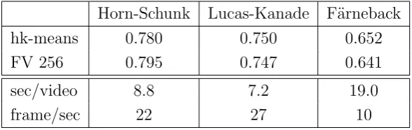
The results reported in the previous section show that both the HOF and the MBH(x/y) descriptors are much more expensive to extract than the HOG descriptors (Table 3.7). This is because calculating the optical flow is computationally expensive. Additionally, not much research has been done on how different optical flow methods affect HOF/MBH descriptors. Therefore in this experiment we evaluate five available optical flow imple-mentations to investigate both their computational efficiency and accuracy. In particular, we compare: (1) Farneb¨ack [28] from OpenCV using the mex-opencv interface, (2) Lucas-Kanade [49] and (3) Horn-Schunk [32] from the Matlab Computer Vision Systems Toolbox, (4) Brox 04 [8] and (5) Brox 11 [9] using the available author’s code.
Results are presented in Tables 2.4 and 2.5. Specifically, while in Ta-ble 2.4 we used the same setting adopted in the other experiments of this work, in Table 2.5 we downscaled the frame resolution of all the videos by a factor of 4 (i.e., using 80 ×60 pixel frames) and we subsampled every 6 frames (see Section 2.4.4). This scale and time subsampling was necessary in order to process our large video dataset with both Brox 04 and Brox 11, two state-of-the-art dense optical flow methods not able to process videos in real time. In fact, processing all the frames of our 6600 videos at full spatial resolution with Brox 11 would require a few months.
Horn-Schunk Lucas-Kanade F¨arneback
hk-means 0.780 0.750 0.652
FV 256 0.795 0.747 0.641
sec/video 8.8 7.2 19.0
frame/sec 22 27 10
Table 2.4: Comparison of different optical flow methods used to compute HOF features. Results obtained with no frame subsampling and at full original spatial resolution (320×
240 pixels).
Horn-Schunk Lucas-Kanade F¨arneback Brox 04 Brox 11
hk-means 0.713 0.681 0.529 0.548 0.552
FV 256 0.718 0.697 0.542 0.638 0.652
sec/video 2.9 2.8 0.76 7.2 12.4
frame/sec 68 69 257 27.4 16
optical flow affects the results by up to 15%(!).
In terms of computational efficiency, Lucas-Kanade is the fastest at 27 frames/second, followed by Horn-Schunk at 22 frames per second, while Farneb¨ack is slower with 10 frames/second. However, while Lucas-Kanade is faster, its trade-off between efficiency and accuracy is not good: As seen in Table 3.7 Horn-Shunk with a frame sampling rate of 2 outperforms the Lukas-Kanade results in Table 2.4 in both speed (33 frames vs 27 frames) and accuracy (0.77 vs 0.75).
Table 2.5 reports results when we subsample frames and reduce the frame size by a factor 4, enabling comparison with the Brox methods. Note that for a fair comparison these times include the computation for reducing the frame sizes (although these times are negligible compared to the total description extraction time). It can be seen that both Brox methods are better than Farneback, but surprisingly not better than the Horn-Shunk and Lucas-Kanade method. One explanation is that this is due to the low resolution of the frames, which makes dense optical flow extraction not sufficiently accurate. Another possibility is that optical flow methods performing better on optical flow benchmarks are not necessarily optimal for use in classification; reducing mistakes in most parts of the flow may introduce artifacts elsewhere that negatively affect results in a classification framework.
In terms of computational efficiency, Brox 11 is the slowest, followed by Brox 04: even subsampled on reduced frames Brox 04 still processes only 27 frames/sec. In contrast to results without downsampling, Farneb¨ack is here the fastest method. Apparently, there is some overhead in the Matlab optical flow implementations.
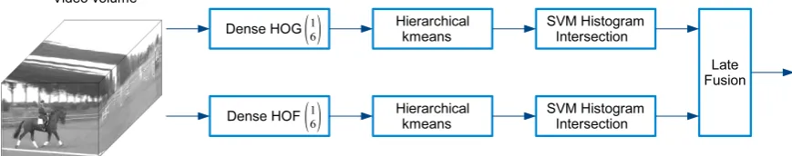
op-Figure 2.7: Recommended pipeline for accurate video classification. This pipeline yields an accuracy of 0.818 on UCF50 while processing 9 frames per second.
Figure 2.8: Recommended pipeline for realtime video classification. This pipeline yields an accuracy of 0.790 on UCF50 while processing 28 frames per second.
2.4.6 Recommendations for practitioners
Based on the results of the previous experiments, we can now give several recommendations when accuracy or computational efficiency is preferred. For calculating Optical Flow, Section 2.4.5 showed that the Matlab im-plementation of Horn-Schunk is always the method of choice. In terms of frame sampling rate, for HOG descriptors we always recommend a sam-pling rate of every 6 frames. For HOF descriptor, if one wants accuracy we recommend a sampling rate of every 2 frames and if one wants com-putational efficiency we recommend a sampling rate of 6. The same holds for MBH(x/y) descriptors. For the word assignment method, the Fisher Vector is the method of choice for accuracy. For computational efficiency there are two candidates: hierarchical k-means and the Random Forest. Observe first that the descriptor extraction time is the most costly phase of the pipeline: Extracting HOF descriptors with a sampling rate of 6 frames takes 3.8 seconds per video to compute. And while the Random Forest is five times faster than hierarchical k-means, the difference is only 0.41 seconds per video, which is very small compared to the descriptor extraction phase. Furthermore, Table 3.2 showed a significant drop of ac-curacy from 0.780 for hierarchical k-means to 0.732 for Random Forests (and a similar drop of accuracy is observed with MBH(x/y)). Therefore we recommend using hierarchical k-means for a fast video classification pipeline.
We found that late fusion of the classifier outputs gave slightly better results than early fusion of the descriptors (e.g. concatenating HOG and HOF). Hence in our recommendations we perform a late fusion with equal weights.
Method Accuracy Wang et al. [86] (2013) 0.856%
This work 0.818%
Reddy et al. [63] (2012) 0.769% Solmaz et al. [75] (2012) 0.737% Everst et al. [26] (2013) 0.729% Kliper-Gross et al. [42] (2012) 0.727% Table 2.6: Comparison with the State-of-the-Art.
descriptors, possibly taking into account the complementarity of appear-ance/motion information of different features, and (2) the fastest solution with a sufficiently good accuracy degree. The final recommended pipelines are visualized in Figures 2.7 and 2.8.
The most accurate pipeline (Figure 2.7) combines all the descriptors we adopted in this work: HOG, HOF, MBHx and MBHy. HOG are ex-tracted using all the frames, while HOF and MBH(x/y) are exex-tracted with a sampling rate of 2. The word assignment method used in this case is the Fisher Vector. Using this pipeline we can process 11 frames per second (for video frames of 320 by 240 pixels) at an accuracy of 0.818 on UCF50. Conversely, our recommended pipeline for computational efficiency (Fig-ure 2.8) is based on late fusion of only HOG and HOF, both extracted with a sampling rate of 6 and using hk-means. This second pipeline can process 28 frames per second at a respectable accuracy of 0.790.
2.4.7 Comparison to state-of-the-art
As can be seen, the method of [86] yields the best results. This method is a combination of Dense Trajectories and STIP features [46]. As our results are better than [46], we expect that a combination of dense trajectories with our method would increase results further. In general, our method yields good performance compared to many recently proposed methods, which shows that we provide a strong implementation of densely sampled HOG, HOF and MBH(x/y) descriptors.
2.5
Conclusion
this work presented an evaluation of the trade-off between computational efficiency and accuracy for video classification using a Bag-of-Words pipeline with HOG, HOF and MBH descriptors. Our first contribution is a strong and fast Matlab implementation of densely sampled HOG, HOF and MBH descriptors, which we make publicly available.
In terms of visual word assignment, the most accurate method is the Fisher Kernel. Hierarchical k-means is more than 6 times faster while yielding an accuracy loss of less than 2% and is the method of choice for a fast video classification pipeline. HOG descriptors can be subsampled every 6 frames with a negligible loss in accuracy, while being 2 times faster. HOF and MBH descriptors can be subsampled every 2 frames with negligible loss in accuracy, being 1.5 - 1.7 times faster. When speed is essential, HOF and MBH descriptors may be subsampled every 6 frames.
Compared to the state-of-the-art, the Dense Trajectory method of [86] obtains better results. Nevertheless, the huge difference for the choice of optical flow methods suggests this would also influence dense trajectories. Furthermore, Dense Trajectories still benefit from a combination with nor-mal HOG, HOF and MBH descriptors [39, 86]. Finally, comparisons with other recent methods on UCF50 shows that we provide a strong implemen-tation of dense HOG, HOF and MBH descriptors to the community.
Chapter 3
Efficient Human Action Recognition
using Histograms of Motion
Gradients and VLAD with
Descriptor Shape Information
1
Feature extraction and encoding represent two of the most crucial steps in an action recognition system. For building a powerful action recogni-tion pipeline it is important that both steps are efficient and in the same time provide reliable performance. This work proposes a new approach for feature extraction and encoding that allows us to obtain real-time frame rate processing for an action recognition system. The motion information represents an important source of information within the video. The com-mon approach to extract the motion information is to compute the optical flow. However, the estimation of optical flow is very demanding in terms of computational cost, in many cases being the most significant processing step within the overall pipeline of the target video analysis application. In
1Duta, I.C.; Uijlings, J.R.R.; Aizawa, K.; Hauptmann, A.G.; Ionescu, B. and Sebe, N.
”Effi-cient Human Action Recognition using Histograms of Motion Gradients and VLAD with
this work we propose an efficient approach to capture the motion infor-mation within the video. Our proposed descriptor, Histograms of Motion Gradients (HMG), is based on a simple temporal and spatial derivation, which captures the changes between two consecutive frames. For the en-coding step a widely adopted method is the Vector of Locally Aggregated Descriptors (VLAD), which is an efficient encoding method, however, it considers only the difference between local descriptors and their centroids. In this work we propose Shape Difference VLAD (SD-VLAD), an encoding method which brings complementary information by using the shape infor-mation within the encoding process. We validated our proposed pipeline for action recognition on three challenging datasets UCF50, UCF101 and HMDB51, and we propose also a real-time framework for action recogni-tion.
3.1
Introduction
Over the recent years an explosive growth in video content has occurred and continues growing. As an example of this fulminant increase, Cisco forecast2 mentioned that the IP video would account for 80% of all IP traffic by 2019. With this huge amount of multimedia content, computational efficiency has become as important as the accuracy of the techniques.
Even though in the past several years there has been an important progress in video analysis techniques, in particular on improving the ac-curacy of human action recognition in videos [86, 88, 70, 82, 51, 52, 87], the current methods in terms of computational time are able to run with 1-3 frames per second. For instance, in [82] is reported that the popular approach in [45] runs with 1.4 frames per second. Fast video analysis is important in many applications and this issue of efficiency became very
important for large-scale video indexing systems or automatic clustering of large video collections.
The Bag of Visual Words (BoVW) framework with its variations [46, 86, 88] has been widely used and showed its effectiveness in video analy-sis challenges. The schematic view for a BoVW pipeline is represented in Fig. 3.1, which contains in general three main steps: feature extraction, feature encoding and classification. In addition to these main steps, the framework contains some pre/post processing techniques, such as PCA, feature decorrelation and normalization, which can influence considerably the performance of the pipeline. The commonly used approach for classifi-cation is employing a fast SVM classifier over the resulted video represen-tations. The encoding step creates a final representation of the video and a very widely used approach is counting the frequency of the visual words. However, recently super-vector based encoding methods, such as Vector of Locally Aggregated Descriptors (VLAD) [36] and Fisher Vector (FV) [61], obtained state-of-the-art results for many tasks.
The video contains two important sources of information: the static information in the frames and the motion between frames. The feature extraction step focuses mainly on these two directions. The first direction has the goal to capture the appearance information in frames, such as His-togram of Oriented Gradients (HOG) [15, 46]. The other direction is based on optical flow fields like Histogram of Optical Flow (HOF) [46] and Motion Boundary Histograms (MBH) [16]. These descriptors are extracted and combined using Space Time Interests Points (STIP) [45], dense sampling [90, 82] or extracting the descriptors along some trajectories [78, 86, 88].
Video volume
Descriptor
Extraction Classification
Descriptor Encoding
Post-processing
Pre-processing
Figure 3.1: The general pipeline for video classification.
method. However, for descriptor extraction and encoding there is still room for improvement. For an efficient video classification system it is necessary that both, descriptor extraction and encoding, to be efficient, otherwise if one of them is not competitive regarding the performance, then the target cannot be reached. As one of the goals of this work is to provide a very efficient system for video classification, we propose new solutions for both steps: descriptor extraction and encoding.
Temporal variation within the videos provides an important source of information about its content. Usually, the temporal information is com-puted with an optical flow method. There is a large number of approaches for extracting the optical flow fields, from relatively classic methods, such as [49, 32] to relatively recent approaches like [28, 8, 97, 9], which use com-plex algorithms to compute the motion information. The main drawback of those methods is the high computational cost. This shortcoming be-comes the bottleneck in many applications. For instance, the authors in [86] report that optical flow takes more than 50% of the total time for fea-ture extraction. We present in this work a new efficient descriptor, called Histograms of Motion Gradients (HMG), which is based on the motion information. The proposed HMG descriptor captures the motion infor-mation using a very fast temporal derivation, which enables us to have similar computational cost as HOG but with a significant improvement in accuracy.
of the research works in computer vision and multimedia [88, 58, 82] the super vector-based encoding methods are shown to outperform the other encoding methods. Vector of Locally Aggregated Descriptors (VLAD) [36] is one of the most popular and efficient super vector-based encoding meth-ods which proved its efficiency in creating the final representation of a video for action recognition tasks. Besides its performance, VLAD has several drawbacks. It considers only the mean to represent a cluster of features and also keeps only the first-order statistics and ignores other source of informa-tion. The mean is not enough to reflect a distribution, but in general, the mean and the standard deviation can be enough to capture the statistics. To address this issue, this work proposes to improve VLAD by keeping the standard deviation information and incorporating shape information as the difference of standard deviations between the altered standard deviation of local descriptors and the standard deviation of the visual word. This new encoding method, Shape Difference for VLAD (SD-VLAD), captures the distribution shape of the features and brings complementary information to the original VLAD.
The main contributions of this work can be summarized with the fol-lowing:
• We introduce a new descriptor (HMG), which captures the motion information using a simple temporal derivation, without the need of using the costly optical flow. We make the code for descriptor extrac-tion available3;
• We propose a new encoding method (SD-VLAD), which captures shape information within the encoding process, providing the best trade-off between accuracy and computational cost. We make the code for descriptor encoding available3;
• We adopt several speed-ups, such as fast aggregation of gradient re-sponses, reuse subregions of aggregated magnitude rere-sponses, and frame subsampling, which make the pipeline more efficient;
• We propose an integration of our descriptor and encoding method in a specifically designed video classification framework which allows for real-time performance while maintaining the high accuracy of the results.
The rest of the chapter is organized as follows. Section 3.2 presents the related work. Section 3.3 introduces our new proposed descriptor with the adopted approaches for improving the efficiency. The new encoding method is presented in Section 3.5.4. The experimental evaluation and the comparison with state-of-the-art are presented in Section 3.5. Finally, Section 3.6 concludes this work.
3.2
Related work
found that dense sampling methods generally outperform interest points, especially on more difficult datasets.
The previously mentioned methods establish the region of extracting for several standard descriptors, such as Histogram of Oriented Gradi-ents (HOG) [15, 46], Histogram of Optical Flow (HOF) [46] and Motion Boundary Histograms (MBH) [16]. The work in [47, 46] considers Spatial Pyramid (SP) approach to capture the information about features loca-tion. The works in [38, 62] focus on improving the efficiency of action recognition by exploring different alternatives for the computation of the standard optical flow.
Recently, the approaches based on Convolutional Neural Networks (CNN) [40, 71, 70, 96, 79, 56, 6] have proven to obtain very competitive results compared to traditional hand-crafted methods. In general, for action recog-nition tasks, these works use the two-stream approach where one network is trained on the static images and another network is trained on the optical flow fields. In the end there is a fusion over the output of both networks to provide the final result. In [25, 20] propose solutions for feature encod-ing specifically designed for deep features. The work in [17] uses a hybrid representation by combining hand-crafted with deep features and takes ad-vantage of different techniques to boost the performance. The work in [93] is fully based on deep features, modeling long-range temporal structure and using a series of good practices to improve the network performance.
and discriminative approaches and aggregates the first- and the second-order statistics. FV is performing a soft assignment which in general gives better performance, however, this affects the computational cost. The work in [43] proposes an extension to Spatial Fisher Vector (SFV) which com-putes per visual word the mean and variance of the 3D spatio-temporal location of the assigned features. VLAD encoding method can be viewed as a simplification of FV which keeps only first-order statistics and per-forms hard assignment, which makes it much faster than FV. SVC method keeps the zero-order and first-order statistics, thus SVC can be seen as a combination between Vector Quantization (VQ) [72] and VLAD.
the encoding process the spatio-temporal information showing a consistent improvement in accuracy.
The work in [2] proposes to use intra-normalization to improve VLAD performance. The impact of this approach is to suppress the negative effect of the high values within the vector, which can dominate the similarity between vectors. The authors propose to L2 normalize the aggregated residuals within each VLAD block. We consider also intra-normalization in our framework. Furthermore, they use vocabulary adaptation as an efficient approach to extend the vocabulary to another dataset. In [1] it is proposed RootSIFT normalization to improve the performance of the framework for object retrieval. This normalization approach is based on the idea to reduce the influence of large bin values, by computing square root of the values.
Frame i
∂t
∂x
∂y
Frame i+1
Motion image
Horizontal image gradient
Vertical image gradient
Figure 3.2: Visualization of the process for capturing the motion information for the HMG descriptor. We initially perform a fast temporal derivation over each two consecutive frames, which provides us the motion image. Then we compute the horizontal and vertical gradients for the resulted motion image. The pixels depicted in blue color represent the negative values after temporal derivation.
extraction and encoding allows us to build a very efficient pipeline for video classification, being able to run at more than real-time frame rate.
3.3
Proposed HMG method for descriptor extraction
In this section we introduce the proposed method for capturing motion information from the video. We present several speed-ups that make the framework very efficient, being able to achieve real-time processing.
3.3.1 Histograms of Motion Gradients (HMG)
the first step of an action recognition framework Fig. 3.1. The illustra-tion of the process of capturing the temporal informaillustra-tion is presented in Fig. 3.2. For each two consecutive frames we first compute the temporal derivation:
T(i,i+1) =
∂(Fi, Fi+1)
∂t (3.1)
where Fi is the frame at time index i.
The temporal derivative is computed very effectively by applying a sim-ple and fast filter window [1 -1] for each two consecutive frames (Fi, Fi+1).
The result of this operation is illustrated in the middle image of Fig. 3.2, where we can observe that the information about the motion between two frames is kept. We can call the output of the applied temporal derivative ”motion image”. Obviously, after applying the temporal derivation some values are negative, depending on the result of derivation between the pix-els in frame i and frame i+ 1, we represent the negative values with blue color in Fig. 3.2.
After the computation of the temporal derivative, we compute the spa-tial gradients of the resulted motion image, which allows us to compute the magnitude and the angle of the gradient responses. In the right part of Fig. 3.2 there are represented the horizontal and vertical gradients, computed with:
X(i,i+1) =
∂T(i,i+1)
∂x , Y(i,i+1) =
∂T(i,i+1)
∂y (3.2)
After we obtain the spatial derivatives, similar as for HOG, we compute the magnitude and the angle:
mag = pX2 +Y2, θ = arctan
Y X
(3.3) where each operation from the above formulas is element-wise.
The result of these operations is a 2-dimensional vector field per each new motion frame. We quantize the orientation (θ) in 8 directions/bins and then we accordingly accumulate the magnitude corresponding to each bin. This is similar to how gradient responses are accumulated in SIFT [48]. The next step is to perform the aggregation of those quantized responses over blocks in both spatial and temporal direction. Then we concatenate the responses over several adjacent blocks. We provide in the next subsec-tion the details about the procedure of dividing the video in blocks and volumes. Afterwords, the pipeline in Fig. 3.1 continues with the next step by applying some pre-processing operations before feature encoding, such as normalization and PCA with decorrelation of features. The next steps after the descriptor extraction are very important for the performance of our descriptor. For instance, the descriptors obtained from the motion im-age may include noise which can result in high peaks that can dominate the entire vector representation. To reduce the negative influence of this aspect, over the initial representation of the descriptors we apply Root-SIFT normalization [1], which penalizes more the high values within the vector, contributing to creating a smoother vector (without large peaks) to represent each local extracted descriptor.
3.3.2 Speed-up HMG extraction
y
x
t
Figure 3.3: The process of dividing the video in blocks and volumes. The part depicted in green represents an illustration of a volume created from 3 by 3 by 2 blocks.
several speed-ups that improve the efficiency of the descriptor extraction process of HMG. The efficiency improvement is performed by taking the advantage of the densely sampled approach and by adopting to our new descriptor several speed-ups presented in [82].
video volume consists of 3 by 3 by 2 blocks, corresponding to x, y and t axis. By choosing the sampling rate equally with the block size, then we can reuse the blocks for making the descriptor extraction efficient. Therefore, the representation for a block is computed only once and then use it for the construction of all the volumes around that block. For instance, each block can be reused for 18 times (excepting the blocks on the borders) for the current size of the video volume: 3 by 3 by 2 blocks.
2) Fast aggregation of responses: After we compute the magnitude and the angle, the resulted responses are aggregated for each block. We adopted the approach in [83]. Basically we compute the aggregation of all the frame pixels by doing just a multiplication of three matrices. After the spatial aggregation of 8 by 8 pixels and the temporal aggregation of 6 frames, each block is characterized by 8 values as we consider 8 orientations for quantization of responses. Having 8 bins and a size of 3 by 3 by 2 for video volume, the original dimensionality of our descriptor is therefore 144.
3) Frame subsampling: For efficiency reasons we evaluate HMG by sub-sampling video frames. Subsequent frames contain redundant information, and the computational cost can be substantially improved by frame sub-sampling. We evaluate the impact on the accuracy and efficiency of our descriptor by skipping frames. A detailed analysis of the trade-off between accuracy and computational time is presented with the experimental re-sults.
3.4
Proposed SD-VLAD method for descriptor
en-coding
3.4.1 VLAD representation
VLAD is initially proposed in [36] and can be seen as a simplification of the FV. For the VLAD pipeline first a codebook of k visual words is learned with k-means, M = {µ1, µ2, ..., µk}, which are the means for each cluster.
For each visual word a subset of local descriptors is assigned based on the nearest neighborhood criterion, Xi = {x1, x2, ..., xni}, where x is a feature
vector and ni is the number of assigned features to the i-th visual word.
The idea of VLAD is to accumulate for each visual word the residuals (the differences between the assigned descriptors and the centroid):
vi = ni
X
j=1
(xj −µi) (3.4)
The final VLAD representation is a concatenation of all vectors vi and
the final dimensionality of VLAD is k × d, where d is the dimension of the descriptors. The VLAD performance can be boosted by using intra-normalization [2], which normalize independently each VLAD block vi:
vi
||vi||p
, usually p = 2 (i.e., the L2 norm).
3.4.2 Shape Difference for VLAD
0 1 2 3 4 5 6 7 8 9 10 11 0
1 2 3 4 5 6 7 8 9 10 11
µ
1
µ
2
first dimension of the features
second dimension of the features
features assigned to µ
1
features assigned to µ2
Figure 3.4: An illustrative example when VLAD fails to provide a reliable representation. Each descriptor is assigned to its nearest centroid, µ1 orµ2. Even though the distribution
of the assigned descriptors to each visual word is completely different, the result of VLAD representation (computed with the standard formula (3.4)) is equal with [1 -8] for both,
v1 and v2. In this case, only the computation of the residuals is not enough for obtaining
![Figure 2.4: Accuracy comparison between [46] and our HOG/HOF descriptors](https://thumb-us.123doks.com/thumbv2/123dok_us/529969.2052923/32.595.130.436.496.568/figure-accuracy-comparison-hog-hof-descriptors.webp)
![Figure 2.5: Computational Efficiency comparison between [46] and our HOG/HOF de-scriptors](https://thumb-us.123doks.com/thumbv2/123dok_us/529969.2052923/33.595.100.508.130.222/figure-computational-eciency-comparison-hog-hof-scriptors.webp)