On the Reduction of Optimization Time in Simulation of Oil Reservoirs

(1)

RESEARCH PAPER

On the Reduction of Optimization Time in Simulation of Oil

Reservoirs

Kaveh Mohammadi, Forough Ameli*

School of Chemical Engineering, petroleum and gas, Iran University of Science and Technology, 16846 Tehran, Iran

*Corresponding Author Email: [email protected] ARTICLE INFO

Article History:

Received 16 April 2019

Revised 30 May 2019 Accepted 14 June 2019

Keywords:

Discretization Optimization Reservoir Simulation Fast-SAGD

ABSTRACT

How to cite this article

Mohammadi K, Ameli F. On the Reduction of Optimization Time in Simulation of Oil Reservoirs. Journal of Oil, Gas and Petrochemical Technology, 2019; 6(1): 39-50. DOI: 10.22034/JOGPT

Thermal recovery techniques including Fast-SAGD process increases

the production efficiency of heavy oil reservoirs. Effective parameters in this study included injection and production rates, height of the injection, production, and offset wells, production and injection cycles, and pressure of the offset wells. In this study, optimization studies were performed. The objective function was defined as the cumulative steam injection to the produced oil to recovery factor. As optimization studies is a time- consuming process, discretized form of effective parameters were applied in this study. Three methods of discretization were selected including linear, square, and logarithmic techniques and their results were compared. In this approach, discretization was based on the results of sensitivity analysis without the exact recognition of the reservoir parameters. Applying this technique, the optimization speed increased three times while the accuracy of the results remained constant. The difference between the optimization results in the continuous and discrete states was less than 3%. Moreover, simulation results of the fast-SAGD process with two cycles were presented in terms of RF, CSOR, temperature and pressure distributions, and the produced oil from SAGD and injected steam to the offset well.

1. INTRODUCTION

Three main classes for EOR techniques include thermal techniques [1, 2], chemical processes [3,

4], and injection methods [5]. For the heavy oil samples, thermal methods are more applicable.

The basis for all these thermal techniques is the

injection of hot fluids which leads to the viscosity reduction. A number of more practical techniques for the thermal recovery include Cyclic Steam Stimulation (CSS), Steam Assisted Gravity Drainage (SAGD), in-Situ Combustion (ISC), and Continuous Steam Injection (CSI). In SAGD method, two horizontal wells are drilled in parallel. The upper well is applied for the steam injection and the lower well is utilized for the oil production. This would be possible as heat is transferred from the upper well

(2)

called Fast-SAGD method [15-19]. This process was simulated by Shin and Polikar [20]. Results revealed that the operating costs increased. More oil was produced in Fast-SAGD process and the cumulative steam to oil ratio (CSOR) was reduced in comparison to SAGD method [21]. An optimization study of fast-SAGD process was also performed by Shin and Polikar [19]. Steam injection pressure, rate of steam injection, and location of offset well were optimized. The oil production rate increased 35% and CSOR value reduced, leading to 24% enhancement in the energy efficiency. The optimum pressure of the edge well was obtained by Jeong et al. [15] using artificial neural network technique. A field scale study was done by Rios et al. [22]. The beginning of the CSS process and its impact on NPV was determined using the sensitivity analysis. Kamari et al. [23] also performed a comparative study on Fast-SAGD and SAGD methods in a fractured reservoir. To completely study the sensitivity analysis, the interaction parameter should be considered. For the complicated problems in petroleum engineering, this might be a time-consuming process.

In this study, discrete form of variables was applied to decrease the optimization run time. Decreasing the search space leads to obtaining the optimum point in a shorter time. One possible problem would be decreasing the accuracy

of the results in comparison to the optimum point of the continuous space. To overcome this obstacle, a systematic approach was applied. To maintain the accuracy of the results, sensitivity analysis was performed. The influence of each variable for the optimization was examined on the objective function using the Minitab software. The optimization variables were then transferred from the continuous to the discrete space. The process was simulated using CMG STARS and optimized by the genetic algorithm.

2. Research Method

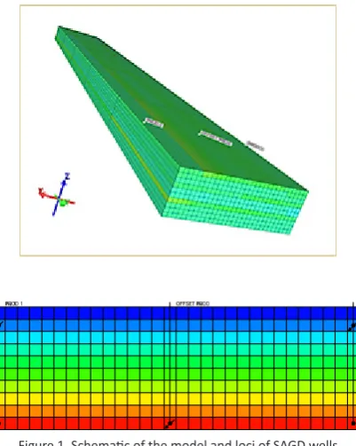
This study was based on Kamari et al. [23] model and consists of 30

×

5

×

10 grid blocks in x,y, and z directions with reservoir size of 150, 1000, and 50 ft, respectively. An offset well and two pairs of injection and production wells were also located in the reservoir. The black oil simulator was applied in CMG STARS. Three pseudo- components were selected for the oil sample characterization namely, CO2–C1, C2–C6, and C7+ with mole fractions of 0.1124, 0.1854, and 0.7022, respectively. The schematic of the model with loci of the SAGD wells is depicted in Figure 1. The characteristics of the Fast-SAGD process are represented in Table 1. The temperature and quality of the injected steam were 600 F and 0.9, respectively. The fluid and rock characteristics are represented in Table 2.

(3)

Table 1. Characteristics of Fast-SAGD process in one-cycle mode [1]

Variable Value

SAGD production well height 4 ft. SAGD injection well height 44 ft. SAGD production well BHP 1100 psi Max SAGD injection well rate 1000 bbl/day Max SAGD injection well pressure 1320 psi Offset well height 4 ft. Offset production well BHP 1100 psi

Soak Time 25 day

Injection onset time 0 month Injection period 6 month

Offset well injection pressure 1950 psi Offset well injection rate 1000 bbl/day

Table 2. Reservoir Rock, Fluid Properties [1]

Parameter Value

Fracture Permeability 2000 md Fracture porosity 0.006% Rock Matrix Porosity 0.195% Matrix Horizontal Permeability 50 md Matrix Vertical Permeability 50 md Matrix Oil Saturation 85% Fracture Oil Saturation 95% Reservoir Pressure 1200 psi Reservoir temperature 140 F Residual Oil Saturation 40% Residual Water Saturation 15%

Viscosity 4000 cp

Formation Thermal Conductivity 24 Btu/day.ft.F Oil Thermal Conductivity 2 Btu/day.ft.F Matrix Heat Capacity 30 Btu/ft^3.F

2.1 Optimization

Genetic algorithm was applied as one of the most practical approaches for optimizing the oil industry problems. Optimization variables included pressure, injection and production rate of offset well, heights of offset and SAGD wells, and injection and production times of the offset well. The objective function of this study was:

Objective function= CSOR/RF

where CSOR represents the ratio of cumulative steam injection to the produced oil and RF stands

(4)

2.2 Discretization

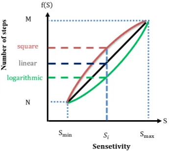
Converting the continuous interval of a variable into several intervals and selecting a point representative of that interval is called discretization.

The number of the nodes is called steps, and the

consecutive distance of each two points is called step length. The discretization leads to increasing the optimization speed. The continuous space for variables x and y is represented as a square. For the discretized form, this space is converted to a number of specified points. The optimum solution may be placed in points other than those are specified in the discretized form. In this case, the actual optimal point would tend to the closest defined point. This would lead to errors in the solution which could be reduced by increasing the discretization steps to an optimum value in terms of the accuracy of the results and run time. For large values of the discretization steps, there is a little difference in the results of continuous and discrete modes and the discretization would not lead to the increased values of speed in the optimization process. As a result, the effect of optimization variables should be defined on the objective function using the empirical and analytical techniques. Empirical techniques are applicable for reservoirs with well-defined characteristics to forecast the reservoir behavior for any variations. For the reservoirs without the fully defined characteristics, analytical approaches are applied to study the model sensitivity to various parameters.

2.2.1 Sensitivity Analysis

In this section, sensitivity analysis of the input parameters is studied for the model outputs. Minitab software was applied for this purpose. A two-level

factorial technique was also applied for defining the number of runs and the analysis of variance for the mathematical analysis of the results.

2.2.2 Defining the number of steps for the discretization

In the next step, a logical connection was established between the sensitivity value for each parameter and the number of steps. For this purpose, three various functions were defined namely, square, logarithmic and linear. These functions are represented as follows [24]:

exp(

)

i i

y

ax

b

y

ax

b

y

ax

b

=

+

=

+

=

+

(1)

These functions are used to define the step number for other parameters using the variables with minimum and maximum effects. In this study, the number of steps allocated to the variables with the least and the most error values were defined as 3 and 20, respectively, using trial and error. Figure 2 represents the number of steps for each function. The minimum number of steps refers to logarithmic function and the maximum number of steps is for the square function. In this section, five cases are considered which are represented in Table 3. Specified values were assigned to the steps of the least and the most values of sensitivity. These are applied for determining the best number of steps for the optimization.

(5)

Table 3. The selected cases for discretization

Min Steps

Max Steps Cases

5

3

Case1

10

3

Case2

20

3

Case3

25 5

Case4

35 10

Case5

2.2.3 Discretization of continuous parameters

Specified number of steps has been calculated using the sensitivity analysis for different cases in Table 3. Variables should be transferred from the continuous to the discrete space. For variable x in the range of 0 to 1, if the number of steps is equal to n, the length of each segment would be:

) 1 ( ) 1

( × −

= _i

i _n n

S (2)

The value of

F

iin a specified segment would

be:

) 1 ( ) 1 1

( × −

−

= _i

i _n n

F (3)

For x in the range of 0 and 1: If :

i i

i

x

S

f

x

F

S

≤

<

+1

→

(

)

=

(4)

Figure 3 represents the discretization of variable x using three steps. In this figure, the values of S are equal to 0, 0.33, 0.66, 1. Moreover, F values are 0, 0.5, and 1. The initial and end point of each range are also considered in the optimization. Therefore, for x between 0 and 0.33, the value of f(x) would be 0, and for the range of 0.33 to 0.66 it would be 0.5. Briefly, using the sensitivity analysis, the effectiveness of each variable on the objective function was determined. Implementing the linear, square, and logarithmic functions, the number of discretization steps would be determined for each of the selected variables. Finally, using the discretization equations, continuous variables were transferred to the discrete space.

Figure 3. Displaying the discretization of variable x using 3 steps

3. Results and Analysis

3.1 Sensitivity Analysis of the model

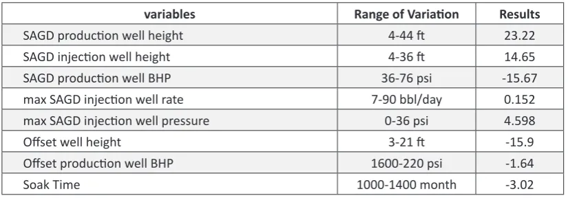
Effectiveness of each of the selected variables is

represented in Table 4 in which various parameters and their effects are shown on the objective function.

Table 4. Sensitivity analysis results

variables Range of Variation Results

SAGD production well height 4-44 ft 23.22 SAGD injection well height 4-36 ft 14.65 SAGD production well BHP 36-76 psi -15.67 max SAGD injection well rate 7-90 bbl/day 0.152 max SAGD injection well pressure 0-36 psi 4.598

Offset well height 3-21 ft -15.9

Offset production well BHP 1600-220 psi -1.64

(6)

Higher values of sensitivity analysis lead to assigning more nodes to the converted discrete variables. The most sensitivity refers to the height of SAGD injection well, and the minimum sensitivity is assigned to the maximum injection rate of SAGD injection well.

3.2 Comparison of different functions with continuous state

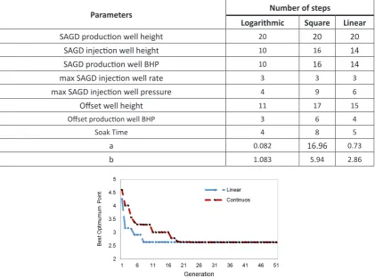
The number of steps allocated to each parameter

in logarithmic, linear, and square functions is reported in Table 5. The maximum number of steps is attributed to the linear function. On the other hand, the logarithmic function introduced the least repetition of the steps. For all cases, the maximum number of the discretization steps is attributed to the height of production well with value of 20 and the minimum number of the discretization steps is for the maximum injection rate for SAGD injection well with the value of 3.

Table 5. The specified number of steps for each of the variables

Number of steps

Parameters

Linear

Square

Logarithmic

20 20

20

SAGD production well height

14

16 10

SAGD injection well height

14 16

10

SAGD production well BHP

3 3

3

max SAGD injection well rate

6 9

4

max SAGD injection well pressure

15 17

11

Offset well height

4 6

3 Offset production well BHP

5 8

4 Soak Time

0.73

16.96

0.082 a

2.86 5.94

1.083 b

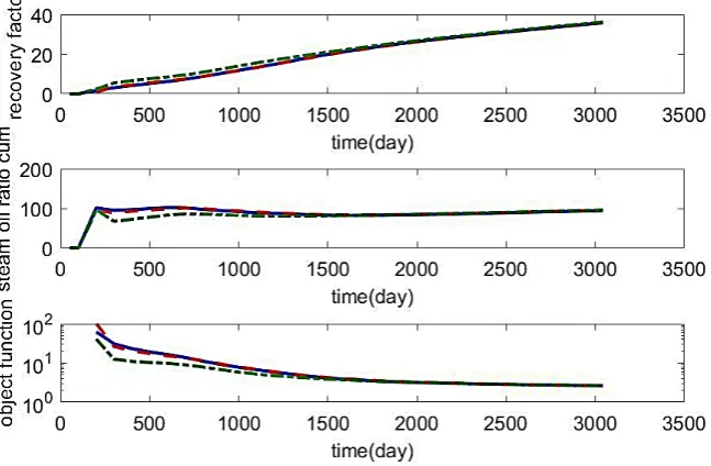
Figure 4. Comparison of the best optimum point in various generations in case 3

Figure 4 represents the accuracy of the results in discretized form for case 3 as the best case in terms of accuracy and the number of repetitions. Values of the best objective functions using the genetic algorithm for the discrete and the continuous states for each generation are represented in this figure. In discrete state, where the linear function was applied to determine the number of steps, results were the same as the continuous state for the least generation. Their difference was

(7)

Table 6. Optimization conditions for the continuous and discrete parameters

Offset production

well BHP (psi) SAGD

production well BHP(psi) Offset

well height

(ft) SAGD

injection well max pressure

(psi) Soak Time

(month) SAGD injection

well max injection rate(bbl/day) SAGD

production well height

(ft) SAGD

injection well height

(ft)

Variable Range 1000-2000

1200-2200 3-21

0-36 0-60

4-44 36-68

4-44

Step Size (x) 100

100 3

3 10

8 8

8

Step Size (2x) 200

200 6

6 20

16 16

16

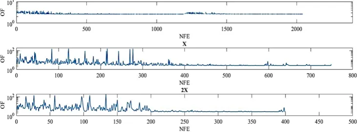
Figure 5 shows the optimization results of the genetic algorithm for the continuous problem and the discretized one with discretization step length of x and 2x. As represented in this figure, the number of function evaluations (NFE) for the continuous state is approximately 2000, while for the discretized states with length of x and 2x, this parameter would be 750, and 400, respectively. This means that the optimization speed for the discrete variables is more in comparison to the continuous state. As most of the recalled data

by the optimization procedure are repetitive, omitting them would increase the optimization speed furthermore. So, not only the number of NFE is reduced, but also the number of saved data in databank would reduce. Figure 6 indicates that for this state, the number of saved data for the continuous and two discrete cases are 2000,360, and 140, respectively. This algorithm would not affect the optimization speed in the continuous state, as all the variables have the same variations.

Figure 5. Results of objective function for the continuous and discrete variables

(8)

To compare the results of the continuous and discrete variables, the recovery factor and CSOR values were compared in various conditions. The error values for each technique were also compared. Figure 7 represents the values of the discrete and continuous parameters for the recovery factor, CSOR, and the recovery factor,

respectively. These curves are depicted for the optimum values. It is inferred from the figures that the discretization error was for the first 1500 days in which the offset well was injected and the pressure and injection rates were different in the various discretization conditions.

Figure 7. Values of the discrete and continuous parameters for the RF, CSOR, and the objective function

Table 7 reports the error values of the recovery

factor and CSOR for the two periods of 5 and 8 years from beginning of the process.

Table 7. Error value for the continuous and discrete parameters

r value for RF in 8 years r value for RF in

5 years r value for CSOR in

8 years r value for CSOR in

5 years

Continuous

1 1

Discrete x 0.9999

0.9991 0.9955

0.9961

Discrete 2x 0.9978

0.9932 0.9385

0.9698

It is inferred from the table that by increasing the step size, the error value would increase. But it is not significant. On the other hand, these results were obtained for the reduced values of NFE.

3.3 Simulation results for the fast-SAGD process with two cycles

In this simulation, the first injection cycle was 18 months, the soak time was 2 months, and the production cycle was 6 months. The second cycle included a 6-month steam injection, a 2-month soak time, and production till the end

(9)

Figure 8. Curves of RF (blue), CSOR (red), and injection cycles in offset well (green)

As the injection pressure of the offset well is more than that of SAGD well, the average reservoir pressure also increased in different injection cycles. In Figure 9, the green and blue curves

are the bottom hole pressure and the average reservoir pressures, respectively. As it is clear, for the injection cycles in offset wells the average reservoir pressure also increased.

.

Figure 9. Effect of the injection pressure in offset well on the reservoir average pressure

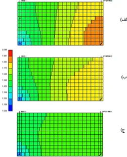
Pressure distribution for the 3rd_{, 6}th_{and 9}th

months after the production are shown in Figure 10. It is clear from this figure that the pressure

front is moving to the SAGD well. The temperature distribution is more uniform in the 12th_month.

(10)

Figure 11 represents the average temperature of the reservoir.

Figure 11. Average reservoir temperature in the injection and production cycles

As the figure clearly shows, the average reservoir

temperature is more for the injection cycles. This is due to the high volume of the injected steam to the reservoir.

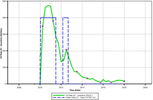
Figure 12. Oil production curve for the produced oil from SAGD well and injected steam to offset well

In addition, as Figure 12 clearly shows for the injection cycles in SAGD well, the produced increases which is due to the high pressure of the injected steam which pushes oil to the SAGD well.

4. Conclusions

1- By applying the new technique, the optimization speed increased three times and the accuracy of the results remained constant. The difference between the optimization results in the continuous and discrete states was less than 3%.

2- In the newly presented approach, the discretization is based on the sensitivity analysis

without the exact recognition of the reservoir parameters. Mathematical analysis was applied to forecast the reservoir behavior and to perform the discretization of the continuous variables.

References

1. Hemmati-Sarapardeh, A., et al., Experimental determination of interfacial tension and miscibility of the CO2–crude oil system; temperature, pressure, and composition effects. Journal of Chemical & Engineering Data, 2013; 59(1): 61-69.

(11)

3. Ayirala, S.C. and D.N. Rao. Comparative evaluation of a new MMP determination technique. in SPE/DOE Symposium on improved oil recovery. Society of Petroleum Engineers; 2006..

4. Namdar Zanganeh, M. and W. Rossen, Optimization of foam enhanced oil recovery: balancing sweep and injectivity. SPE Reservoir Evaluation & Engineering, 2013; 16(01): 51-59.

5. Hashemi-Kiasari, H., et al., Effect of operational parameters on SAGD performance in a dip heterogeneous fractured reservoir. Fuel, 2014; 122: 82-93.

6. Deutsch, C. and J. McLennan, Guide to SAGD (steam assisted gravity drainage) reservoir characterization using geostatistics. Centre for Computational Excellence (CCG), Guidebook Series Vol. 3, University of Alberta, April 2003, 2005.

7. Austad, T., Water-based EOR in carbonates and sandstones: new chemical understanding of the EOR potential using smart water. Enhanced Oil Recovery Field Case Studies, 2013: 301-335.

8. Gates, I.D., et al. Steam injection strategy and energetics of steam-assisted gravity drainage. in SPE International Thermal Operations and Heavy Oil Symposium. Society of Petroleum Engineers; 2005.

9. Gates, I.D. and S.R. Larter, Energy efficiency and emissions intensity of SAGD. Fuel; 2014. 115: 706-713.

10. Kam, D., et al., An optimal operation strategy of injection pressures in solvent-aided thermal recovery for viscous oil in sedimentary reservoirs. Petroleum Science and Technology; 2013. 31(22): 2378-2387.

11. Coskuner, G., A new process combining cyclic steam stimulation and steam-assisted gravity drainage: Hybrid SAGD. Journal of Canadian Petroleum Technology, 2009; 48(01): 8-13.

12. Ghanbari, E., et al. Improving SAGD performance combining with CSS. in International Petroleum Technology Conference. International Petroleum Technology Conference; 2011.

13. Li, D.D. and M.L. Greenfield, High internal energies of proposed asphaltene structures. Energy & Fuels; 2011. 25(8): 3698-3705.

14. Xu, J., et al. Numerical thermal simulation and optimization of hybrid CSS/SAGD process in Long Lake with

lean zones. in SPE Heavy Oil Conference-Canada. Society of Petroleum Engineers; 2014.

15. Jeong, S., et al. Optimal Operation of Fast-SAGD Process Considering Steam Channeling among Vapor Chambers. in The Twenty-third International Offshore and Polar Engineering Conference. International Society of Offshore and Polar Engineers; 2013.

16. Kamari, A., et al., New tools predict monoethylene glycol injection rate for natural gas hydrate inhibition. Journal of Loss Prevention in the Process Industries, 2015; 33: 222-231.

17. Polikar, M., T. Cyr, and R. Coates. Fast-SAGD: half the wells and 30% less steam. in SPE/CIM International Conference on Horizontal Well Technology. Society of Petroleum Engineers; 2000. 18. Sarapardeh, A., et al. Application of fast-SAGD in naturally fractured heavy oil reservoirs: A case study. in SPE middle east oil and gas show and conference. Society of Petroleum Engineers; 2013.

19. Shin, H. and M. Polikar, Review of reservoir parameters to optimize SAGD and Fast-SAGD operating conditions. Journal of Canadian Petroleum Technology, 2007; 46(01).

20. Shin, H. and M. Polikar, Fast-SAGD application in the Alberta oil sands areas. Journal of Canadian Petroleum Technology, 2006; 45(09).

21. Shin, H. and M. Polikar. Experimental investigation of the fast-SAGD process. in Canadian International Petroleum Conference. Petroleum Society of Canada; 2006.

22. Rios, V.D.S., P. Laboissiere, and O.V. Trevisan. Economic Evaluation of Nitrogen Injection on SAGD Process. in SPE Latin American and Caribbean Petroleum Engineering Conference. Society of Petroleum Engineers; 2010.

23. Kamari, A., et al., On the evaluation of Fast-SAGD process in naturally fractured heavy oil reservoir. Fuel; 2015; 143: 155-164.

(12)

یتاقیقحت هلاقم

یتفن نزاخم یزاس هیبش رد یزاس هنیهب نامز شهاک

*

یلماع غورف ،یدمحم هواک

ناریا ،نارهت ،16846 یتسپ دک ،ناریا تعنص و ملع هاگشناد ،زاگ و تفن ،یمیش یسدنهم هدکشناد

هدیکچ

هلاقم تاصخشم

Fast-SAGD

دنیارف لماش تفن دیلوت شیازفا یترارح یاهکینکت

رد .دوش یم نیگنس تفن نزاخم رد دیلوت یرو هرهب شیازفا هب رجنم