R E S E A R C H
Open Access
A generalization of the compression cone
method for integral operators with changing
sign kernel functions
Ankai Liu
1and Wenying Feng
2**Correspondence:[email protected] 2Departments of Mathematics and
Computing & Information Systems, Trent University, Peterborough, Canada
Full list of author information is available at the end of the article
Abstract
In this paper, a new class of order cones in the space of continuous functions is introduced. The result unifies some previous work in studying the existence of solutions for differential equations using the compression cone techniques and fixed point theorems. It is shown that the method is more adaptable, particularly in dealing with changing sign Green’s functions. Applications are illustrated by examples. Limitations of such a new method are also discussed.
Keywords: Boundary value problem; Cone; Existence of solutions; Fixed point index; Green’s function; Integral equation; Kernel function
1 Introduction
Recently, it has been shown that the following Hammerstein integral equation has impor-tant applications in the rapidly developing field of machine learning [2]:
Nu(s) := T
0
g(t,s)fs,u(s)ds. (1)
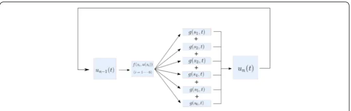
In fact, existence of fixed points for (1) has interesting applications in computing sys-tems. As shown in Fig.1,g is a continuous impulse response,uis the continuous out-put, andf is a controller that generates continuous input from the previous feedback. Convergence of the system is governed by fixed points of the corresponding integral op-erator. Other applications of the integral equation include models of a chemical reactor [7], a thermostat [23], and circuit design [3].
It is known that equation (1) can be seen as an inverse of a differential equation subject to certain boundary conditions. The Green’s function of the boundary value problem (BVP) becomes the kernel of the integral operator. The so-called “compression cone” principle can be used to study existence of fixed points for the integral equation, and therefore the conclusion of existence of solutions for the BVP. For some recent work in higher-order BVPs, we refer to [5,16,20,27] and the references therein. First, the definition of order cone in an abstract Banach space is given below.
Definition 1.1([25], p. 276) LetXbe a Banach space andKbe a subset ofX. ThenKis called an order cone iff:
Figure 1Iterative machine learningun(t) =
Ωg(s,t)f(s,un–1(s))ds
(i) Kis closed, nonempty, andK={0}; (ii) a,b∈R,a,b≥0,x,y∈K⇒ax+by∈K; (iii) x∈Kand–x∈K⇒x= 0.
As a typical example, the following well-known Guo–Krasnoselskii’s fixed point theo-rem is a result of cone compression and expansion.
Theorem 1.2([10]) Let K⊂X be a cone of the real Banach space X.Suppose thatΩ1and
Ω2are two bounded open sets in X such thatθ∈Ω1andΩ1⊂Ω2.Let T:K∩(Ω2\Ω1)→
K be completely continuous.If either
(a) Tx ≤ x forx∈K∩∂Ω1and Tx ≥ x forx∈K∩∂Ω2,or
(b) Tx ≤ x forx∈K∩∂Ω2and Tx ≥ x forx∈K∩∂Ω1
holds,then T has at least one fixed point in K∩(Ω2\Ω1).
To construct the cone in a space such asC[0,T], usually a positive Green’s function for the BVP is required to ensure a positive kernel for the integral operator. Consequently, it leads to existence of positive solutions for the original BVP [12,17,21,23,24,26]. Chang-ing sign solutions have drawn relatively less attention. In the literature [13,14,22], Webb and Infante proved the existence of changing sign solutions when the Green’s function is only positive in a subinterval so that the cone can be defined as follows:
KWI:=
u∈C[0,T] : min
t∈[a,b]u(t)≥δ u
,
whereδ> 0 is obtained from the Green’s function. In [18], Ma used the following cone for changing sign Green’s functions:
KM:=
u∈C[0,T] :u(t)≥0∀t∈[0,T], T
0
u(t)dt≥δ u .
Generally speaking, comparing to positive Green’s functions, it is more difficult to con-struct a suitable cone when the kernel of the integral operator is not positive. In this paper, a bounded linear functionalLis used to define a new type of cones in dealing with chang-ing sign Green’s functions for differential equations:
The idea of construction is a generalization of the previous work. For example,KMcan be directly obtained by takingL(u) =0Tu(t)dt, whileKWIcan be written as union of a family
of cones defined as (2)
KWI=
τ∈[a,b]
Kτ,
whereKτ={u∈C[0,T] :Lτ(u)≥δ u }andLτ(u) =u(τ).
The new class of cones allows us to deal with differential equations with broader types of Green’s functions. Roughly speaking, instead of requiring an upper bound and a lower bound for a given Green’s function, suchLintroduces a different measurement with partial order. We only require Green’s functions to be ‘positive’ in the sense of the new measure-ment.
Applying the generalized cone and fixed point index theory, we obtain new existence results of (1). The sub-linear and super-linear cases are also discussed along with examples to illustrate their applications.
2 Main result
Consider the existence of a fixed point for the integral equation
Nu(s) := T
0
g(t,s)fs,u(s)ds,
whereu∈C[0,T] with standard norm u =maxt∈[0,T]{|u(t)|}.
LetLbe a collection of bounded linear functionalsL:C[0,T]→Rwith norm L ∗= max{u∈C[0,1],u=1}{|Lu|}. We will use the following two sets of assumptions for the kernelg and the nonlinear functionf respectively.
(H1) Assume thatg: [0,T]×[0,T]→Ris continuous and satisfies the Lipschitz
condi-tion with respect tos. There exist a non-trivialL∈L, positive measurable function
Ωwith0TΩ(s)ds<∞, and a constantδ> 0such that, for any givens∗∈[0,T], (H1a) maxt∈[0,T]{|g(t,s∗)|} ≤Ω(s∗);
(H1b) δΩ(s∗)≤k(s∗), wherekis defined ask(s∗) =Lg(t,s∗).
(H2) Assume thatf : [0,T]×R→R+is continuous andM=T1 0 k(s)ds
.
(H2a) There exists0 <r<∞such thatinf0≤t≤T
–r≤x≤r{f(t,x)} ≥ L ∗rM. (H2b) There exists0 <R<∞,R=r, such thatsup0≤t≤T
–R≤x≤R{f(t,x)}<
δRM.
Denote
K:=u∈C[0,T] :L(u)≥δ u , Kr:=u∈C[0,T] :L(u)≥δ u , u ≤r.
It is clear thatKr⊆K⊆C[0,T]. We will prove thatKis a convex cone ofC[0,T]. Further-more, chooseQ>max{r,R}to be large enough, definef˜: [0,T]×R→R+
˜
f(t,x) = ⎧ ⎪ ⎪ ⎨ ⎪ ⎪ ⎩
f(t,x) |x| ≤Q,
f(t,Q) x>Q,
Sincef is continuous,f˜is clearly bounded. DefineN˜ =0Tg(t,s)f˜(s,u(s))ds. The main re-sult is given below.
Theorem 2.1 If(H1), (H2)are satisfied,and
T
0 Lg(t,s)ds> 0,then N has at least one
non-trivial fixed point.
To prove Theorem2.1, we have the following Lemmas2.2,2.3, and2.4from the prop-erties of fixed point index [8]. LetKbe a cone in a Banach spaceX.
Lemma 2.2 If there exists e∈K\{0}s.t.x=Nx+λe for all x∈∂KRand allλ> 0,then the fixed point index i(N,KR,K) = 0 [13].
Lemma 2.3 Let N:K→K be a completely continuous mapping.If Nu=μu for all u∈∂Kr and allμ≥1,then the fixed point index i(N,Kr,K) = 1 [6].
Lemma 2.4 Let P be an open set and N:P→S be a compact mapping.If i(N,P,S)= 0, then N has at least one fixed point in P[15].
In addition, the new Lemma2.5shows thatf˜carries out the same fixed point properties as those off.
Lemma 2.5 If f satisfies the conditions of(H2),then the correspondingf also satisfies˜ (H2).
Moreover,for any u∈C[0, 1]such thatN(u) =˜ u,if u ≤Q,it also satisfies N(u) =u.
Proof From (H2),f˜clearly is continuous on [0,T]×R. For (H2a), we have
inf
0≤t≤T
–r≤x≤r ˜
f(t,x)= inf
0≤t≤T
–r≤x≤r
f(t,x)≥ L ∗rM.
Therefore (H2a) is also satisfied byf˜. The same argument can be made on (H2b).
Lemma 2.6 If(H1)is satisfied,k defined in(H1)is Lipschitz continuous.
Proof For any givens,s∗∈[0,T],
k(s) –ks∗=Lg(t,s) –gt,s∗≤ L ∗g(t,s) –gt,s∗≤ L ∗cs–s∗.
Thusk(s) is also Lipschitz continuous.
The proof of Theorem2.1relies on interchanging two bounded linear operators. We first give Fubini’s theorem and the Riesz representation theorem for the proof of Lemma2.9.
Theorem 2.7(Fubini’s theorem [1]) Let g∈Ω1×Ω2→Rbe a measurable function such
that
Ω1×Ω2
g(ω1,ω2)dP<∞,
whereP=P1×P2.Then
(b) For almost allω2∈Ω2,g(ω1,ω2)is an integrable function ofω1.
(c) There exists an integrable functionh:Ω1→Rsuch that
Ω2g(ω1,ω2)dP2=h(ω1) a.s. (i.e.,except for a set ofω1of zeroP1-measure for which
Ω2g(ω1,ω2)dP2is
undefined or finite).
(d) There exists an integrable functionh:Ω2→Rsuch that
Ω1g(ω1,ω2)dP2=h(ω2) a.s. (i.e.,except for a set ofω1of zeroP2-measure for which
Ω1g(ω1,ω2)dP2is
undefined or finite).
(e) We have
Ω1
Ω2
g(ω1,ω2)dP2
dP1=
Ω2
Ω1
g(ω1,ω2)dP1
dP2
=
Ω1×Ω2
g(ω1,ω2)dP.
Theorem 2.8(Riesz representation theorem [19]) A functional F defined on C[a,b]is lin-ear and continuous if and only if there exists a function g∈BV (bounded variation func-tion)such that
F(f) = b
a
f dg for f∈C[a,b].
Lemma 2.9 Assume that(H1)and(H2)are satisfied.Let L,k be defined as in(H1),then
L
T
0
g(t,s)f˜s,u(s)ds
= T
0
Lg(t,s)˜fs,u(s)ds= T
0
k(s)f˜s,u(s)ds.
Proof SinceLis a continuous linear functional defined onC[0,T], by the Riesz represen-tation theorem, there exists uniqueω∈BV such that0Th(t)dω(t) =L(h). We know that g(t,s) andf˜(s,u(s)) are absolutely bounded for alls,t∈[0,T]. Thus
[0,T]×[0,T]
g(s,t)f˜s,u(s)ds,ω(t)<∞.
By Fubini’s theorem,
L
T
0
g(t,s)f˜s,u(s)ds = T 0 T 0
g(t,s)f˜s,u(s)ds dω(t)
= T
0
T
0
g(t,s)dω(t)f˜s,u(s)ds
= T
0
Lg(t,s)˜fs,u(s)ds (∗)
= T
0
k(s)f˜s,u(s)ds.
For (∗), since for alls∗∈[0,T],g(·,s∗)∈C[0, 1], and so0Tg(t,s∗)dΩ(t) =L(g(t,s∗)). There-fore
max
s∈[0,T]
T
0
g(t,s)dω(t) –Lg(t,s) = 0,
Lemma 2.10 If(H1)and(H2)are satisfied,K defined in(H2)is a cone andN(K)˜ ⊆K.
Proof We first show thatKis a cone. Letu1,u2∈Kand 0≤a,b∈R.
L(au1+bu2) =aL(u1) +bL(u2)≥aδ u1 +bδ u2 =δ au1 +δ bu2 ≥δ au1+bu2 .
Ifu1and –u1∈K, then 0 =L(u1) + (–L(u1))≥2δ u1 , which meansu1= 0. Clearly, for all
givens∗∈[0,T],
Lgt,s∗=ks∗≥δΩs∗≥δ max
t∈[0,T]
gt,s∗|=δ g .
SoKis not empty. Let{ui} →ube an arbitrary convergent sequence inK. SinceC[0,T] is a Banach space, thusu∈C[0,T]. Also, because sequences{L(ui)} →Luand{δ ui } →
δ u , we obtain
L(u) –δ u = lim
i→∞L(ui) –δ ui ≥ilim→∞0 = 0.
This shows thatKis a well-defined cone. We next show thatN(K)˜ ⊆K. Letu∈K, clearly
˜
Nu∈C[0,T] and
L(Nu) =˜ T
0
Lg(t,s)f˜s,u(s)ds (By Lemma2.9)
= T
0
k(s)f˜s,u(s)ds
≥
T
0
δΩ(s)f˜s,u(s)ds
≥δ
T
0
max
t∈[0,T]
g(t,s)˜fs,u(s)ds=δ ˜Nu .
SoN(K)˜ ⊆K.
For compactness. The idea is similar to [13]. We seeN(u) =˜ P◦h(u) as a composition of a compact operatorP(u) =0Tg(t,s)u(s)dsand a continuous operatorh(u) =f˜(s,u(s)). It can be shown thatP(u) is compact using Arzela–Ascoli theorem.
Proof of Theorem2.1 We will prove it in two steps. (1) With Lemma2.2, we will find a subset with index 0. (2) With Lemma2.3, we will find a subset with index 1.
Assume that (H1), (H2a) are satisfied. Consideru∈∂Krif there existsu=Nu˜ that is already a fixed point ofu=N(u) with˜ u =r. Otherwise, by (H2a), we have
˜
fs,u(s)|s∈[0,T]≥ inf 0≤t≤T
–r≤u≤r ˜
f(t,u)≥ L ∗rM.
So
L(Nu) =˜ L
T
0
= T
0
Lg(t,s)f˜s,u(s)ds
= T
0
k(s)f˜s,u(s)ds
≥
T
0
k(s) L ∗rM ds
= L ∗r= L ∗ u ≥L(u).
Lete=g(t,s∗) for somes∗∈[0,T] such thatg(t,s∗)= 0. Clearlye∈K and if there exist u∈∂Kr,λ> 0 such thatNu˜ +λe=u, then
L(u) =L(Nu) +˜ λL(e)
=L(Nu) +˜ λLgt,s∗
≥L(Nu) +˜ λδ g
>L(Nu),˜
which is a contradiction. By Lemma2.2,i(N,˜ Kr,K) = 0. Assume that (H1), (H2b) are satis-fied. Consideru∈∂KR. If there existsu=Nu, then that is already a fixed point of˜ u=N(u)˜ with u =R. Otherwise, by (H2b) we have
˜
fs,u(s)|s∈[0,1]≤ sup 0≤t≤T
–R≤u≤R ˜
f(t,u)<δRM.
Therefore,
L(Nu) =˜ T
0
k(s)f˜s,u(s)ds
< T
0
k(s)δRM ds
=δR=δ u ≤L(u).
If there existu∈∂KR,μ≥1 such thatNu˜ =μu, thenL(Nu) =˜ L(μu)≥L(u), which is a contradiction. By Lemma2.3,i(N,˜ KR,K) = 1.
SinceN˜ has no fixed point at∂Krand∂KR, using the properties of fixed point index, if r>R,
i(N,˜ Kr¯\KR,K) =i(N,˜ Kr,K) –i(N,˜ KR,K) = –1,
by Lemma2.4,N˜ has at least one non-trivial solution inKr\KR. On the other hand, ifR>r,
i(N,˜ KR¯\Kr,K) =i(N,˜ KR,K) –i(N,˜ Kr,K) = 1.
Again by Lemma2.4,N˜ has at least one non-trivial solution inKR\Kr.
3 Sub-linear and super-linear case
Assumptions (H2a) and (H2b) of Theorem2.1can be simplified when the nonlinear part
is in sub-linear or super-linear cases [4]. We introduce the following new conditions for Theorem3.1.
(H3) Assume thatf : [0,T]×R→R+is continuous,M=T 1 0 k(s)ds
,KandKras defined
in(H2).
(H3a) 0 <lim|x|→0inft∈[0,T]f(t,x),
(H3b) 0≤f∞<δM, where
f∞= lim
x→∞
sup
t∈[0,T]
f(t,x)
|x|
.
Theorem 3.1 If(H1), (H3)are satisfied,and
T
0 Lg(t,s)ds> 0,then the integral equation
N has at least one non-trivial fixed point.
Proof Let (H3a) be satisfied, we have 0 <lim|x|→0inft∈[0,T]f(t,x). Then there existm1> 0
andr0> 0 small enough such that
inf
0≤t≤T
|x|≤r0
f(t,x)≥ L ∗Mm1.
Letr=min{m1,r0}, thereforer≤m1andr≤r0. And we can have
inf
0≤t≤T
|x|≤r
f(t,x)≥ inf
0≤t≤T
|x|≤r0
f(t,x)
≥ L ∗Mm1
= L ∗Mr,
which satisfy (H2a).
For the other part, let (H3b) be satisfied, we have 0≤f∞<δM. There existsR0> 0 large
enough such thatsup0≤t≤T
|x|≥R0
f(t,x)
|x| <δM.
Sincef(t,x) is continuous, sof(t,x)||x|<R0is bounded. Letsup0≤t≤T |x|≤R0
f(t,x)≤ ¯B. Assuming
(H3a) is not true, then for anyR> 0,
sup
0≤t≤T
–R≤x≤R
f(t,x)>δRM.
ChooseR>max{R0,δBM¯ }, thereforeR>R0andR>δBM¯ . Since
sup
0≤t≤T
|x|≤R0
f(t,x)≤ ¯B≤δMR,
we have
sup
0≤t≤T R0≤|x|≤R
f(t,x) = sup
0≤t≤T
|x|≤R
and so
sup
0≤t≤T
|x|≥R0
f(t,x)
|x| ≥ 0≤supt≤T R0≤|x|≤R
f(t,x)
|x| ≥ 0sup≤t≤T R0≤|x|≤R
f(t,x) R =δM,
which is a contradiction. Thus (H3b) has to be satisfied. Since (H1), (H2) are satisfied and
T
0 Lg(t,s)ds> 0, by Theorem2.1,Nhas at least one non-trivial fixed point.
4 Examples
Consider the periodic boundary value problem [9,11,18,28]:
⎧ ⎪ ⎪ ⎨ ⎪ ⎪ ⎩
–u(t) –ρ2u(t) =f(t,u(t)) t∈[0,T], u(0) =u(T),
u(0) =u(T).
Whenρ∈/Nis a positive constant, this BVP is equivalent to
u(t) = T
0
G(t,s)fs,u(s)ds,
where a Green’s function is given as
G(t,s) = ⎧ ⎨ ⎩
–sin(ρ(t2–ρs(1–))+sincosρρ(TT)–(t–s)) 0≤s≤t≤T, –sin(ρ(s2–ρt(1–))+sincosρρ(TT)–(s–t)) 0≤t≤s≤T.
Example4.1 Letρ=23,T= 2π, we have the following BVP: ⎧
⎪ ⎪ ⎨ ⎪ ⎪ ⎩
–u(t) –49u(t) =f(t,u(t)) t∈[0, 2π], u(0) =u(2π),
u(0) =u(2π),
wheref(t,x) =e–x22(1 +sin(t)) and the Green’s function changes sign. If we letLg(t,s) =
2π
0 –g(t,s)dt, clearlyLg(t,s) = 2.25 for alls∈[0, 2π]. Alsomaxs,t∈[0,2π]{|g(t,s)|}=
√
3 2 .
Se-lectΩ(s) =
√
3
2 andδ= 1.5
√
3 which satisfy all conditions (H1). The corresponding cone is
defined as
K1=u∈C[0, 2π] :
2π
0
–u(t)dt≥1.5√3 u }.
As for the nonlinear part,f is clearly a continuous positive function. We can calculate that
lim|x|→0inft∈[0,2π]f(t,x) = 3, so (H3a) is satisfied. Moreover, since M=92π, f∞ = 0 <δM,
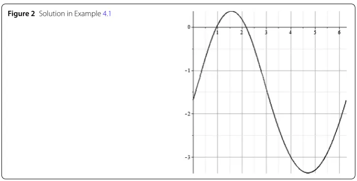
(H3b) is satisfied. Therefore, by Theorem3.1, there exists a non-trivial solution inK1.
Figure2shows the approximation (with 1000 sample points) of the fixed point which was directly obtained from the differential equation. By direct computation we haveLu–
Figure 2Solution in Example4.1
Example4.2 Letρ=14,T= 2π, the period boundary value problem has the form ⎧
⎪ ⎪ ⎨ ⎪ ⎪ ⎩
–u(t) –161u(t) =f(t,u(t)) t∈[0, 2π], u(0) =u(2π),
u(0) =u(2π),
where
f(t,x) = 2cos(2t) x2+ 1 +π.
In this case, the Green’s function is negative. Let Lg(t,s) = –g(π,s), we can show that Lg(t,s)∈[2, 2√2] for alls∈[0, 2π]. We also havemaxs∈[0,2π]{|g(t,s)|}= 2
√
2. LetΩ(s) = 2√2 andδ=√2
2 . All conditions of (H1) are satisfied. Define the corresponding cone
K2=u∈C[0, 2π] : –u(π)≥2
√
2 u }.
As for the nonlinear part,f is clearly a continuous positive function. We can seef(t,x)≥
23
32, so (H3a) is satisfied. We also have M= 1
16π,f∞= 1
32 <δM, so (H3b) is satisfied. By
Theorem3.1, there exists a non-trivial solution inK2.
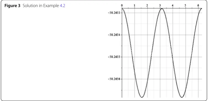
Figure3shows the approximation (with 1000 sample points) of the fixed point which was directly obtained from the differential equation. By direct computation we haveLu–
δ u ≈1.464 > 0, which suggests that it is a fixed point inK2.
We point out that results from [6,13,14,18,22,23] are not applicable to the Green’s functions in the above two examples. The cone applied in [9] and [28]
K=
u∈C[0,T] :u≥0, T
0
u(s)ds≥δ u
Figure 3Solution in Example4.2
Remark4.3 Consider the following example:
g(t,s) = ⎧ ⎨ ⎩
sin(t–s) 0≤s≤t≤2π,
sin(s–t) 0≤t≤s≤2π.
Sinceg(t, 0) +g(t, 2π) = 0 for allt, our method has failed to apply when the Green’s function is reflexive.
Acknowledgements
The authors would like to thank the referees for valuable comments. Support from the Natural Sciences and Engineering Research Council of Canada (NSERC) is greatly acknowledged.
Funding
The project was supported by the Natural Sciences and Engineering Research Council of Canada (NSERC).
Availability of data and materials Not applicable.
Competing interests
The authors declare that they have no competing interests.
Authors’ contributions
Both authors read and approved the final manuscript.
Author details
1Department of Mathematics, Queen’s University, Kingston, Canada.2Departments of Mathematics and Computing &
Information Systems, Trent University, Peterborough, Canada.
Publisher’s Note
Springer Nature remains neutral with regard to jurisdictional claims in published maps and institutional affiliations.
Received: 20 September 2018 Accepted: 7 April 2019
References
1. Adams, M., Victor, G.: Measure Theory and Probability (1996).https://doi.org/10.1007/978-1-4612-0779-5 2. Banka, N., Piaskowy, W.T., Garbini, J., Devasia, S.: Iterative Machine Learning for Precision Trajectory Tracking with
Series Elastic Actuators. CoRR (2017).https://doi.org/10.1109/AMC.2019.8371094
3. Buscarino, A., Fortuna, L., Frasca, M., Sciuto, G.: A Concise Guide to Chaotic Electronic Circuits. Springer, Berlin (2014). https://doi.org/10.1007/978-3-319-05900-6
4. Cabada, A., Lopez-Somoza, L., Tojo, F.A.F.: Existence of solutions of integral equations with asymptotic conditions. Nonlinear Anal., Real World Appl.42, 140–159 (2018).https://doi.org/10.1016/j.nonrwa.2017.12.009
6. Feng, W.: Topological methods on solvability, multiplicity and bifurcation of a nonlinear fractional boundary value problem. Electron. J. Qual. Theory Differ. Equ.2015, 70 (2015).https://doi.org/10.14232/ejqtde.2015.1.70 7. Feng, W., Zhang, G., Chai, Y.: Existence of positive solutions for second order differential equations arising from
chemical reactor theory. In: Discrete Contin. Dyn. Syst., Dynamical Systems and Differential Equations. Proceedings of the 6th AIMS International Conference, pp. 373–381 (2007)
8. Furi, M., Pera, M.P., Spadini, M.: On the uniqueness of the fixed point index on differentiable manifolds. Fixed Point Theory Appl.2004478686 (2004).https://doi.org/10.1155/S168718200
9. Graef, J.R., Kong, L., Wang, H.: A periodic boundary value problem with vanishing Green’s function. Appl. Math. Lett.
21(2), 176–180 (2008).https://doi.org/10.1016/j.aml.2007.02.019
10. Guo, D., Lakshmikantham, V.: Nonlinear Problems in Abstract Cones. Academic Press, San Diego (1988)
11. Hai, D.D.: On a superlinear periodic boundary value problem with vanishing Green’s function. Electron. J. Qual. Theory Differ. Equ.2016, 55 (2016).https://doi.org/10.14232/ejqtde.2016.1.55
12. He, J., Liu, X., Chen, H.: Existence of positive solutions for a high order fractional differential equation integral boundary value problem with changing sign nonlinearity. Adv. Differ. Equ.2018, 49 (2018).
https://doi.org/10.1186/s13662-018-1465-6
13. Infante, G., Webb, J.R.L.: Three Point boundary value problems with solutions that change sign. J. Integral Equ. Appl.
15(1), 37–57 (2003).https://doi.org/10.1216/jiea/1181074944
14. Infante, G., Webb, J.R.: Loss of positivity in a nonlinear scalar heat equation. Nonlinear Differ. Equ. Appl.13(2), 249–261 (2006).https://doi.org/10.1007/s00030-005-0039-y
15. Leggett, R.W., Williams, L.R.: Multiple positive fixed points of nonlinear operators on ordered Banach spaces. Indiana Univ. Math. J.28, 673–688 (1979)
16. Li, P., Feng, M., Wang, M.: A class of singular n-dimensional impulsive Neumann systems. Adv. Differ. Equ.2018, 100 (2018).https://doi.org/10.1186/s13662-018-1558-2
17. Liu, X., Liu, L., Wu, Y.: Existence of positive solutions for a singular nonlinear fractional differential equation with integral boundary conditions involving fractional derivatives. Bound. Value Probl.2018, 24 (2018).
https://doi.org/10.1186/s13661-018-0943-9
18. Ma, R.: Nonlinear periodic boundary value problems with sign-changing Green’s function. Nonlinear Anal., Theory Methods Appl.74(5), 1714–1720 (2011).https://doi.org/10.1016/j.na.2010.10.043
19. Narkawicz, A.: A formal proof of the Riesz representation theorem. J. Formaliz. Reason.4(1), 1–24 (2011)
20. Pei, M., Wang, L., Lv, X.: Existence and multiplicity of positive solutions of a one-dimensional mean curvature equation in Minkowski space. Bound. Value Probl.2018, 43 (2018).https://doi.org/10.1186/s13661-018-0963-5
21. Qian, Y., Zhou, Z.: Existence of positive solutions of singular fractional differential equations with infinite-point boundary conditions. Adv. Differ. Equ.2017, 8 (2017).https://doi.org/10.1186/s13662-016-1042-9
22. Webb, J.R.: Solutions of nonlinear equations in cones and positive linear operators. J. Lond. Math. Soc.82(2), 420–436 (2010).https://doi.org/10.1112/jlms/jdq037
23. Webb, J.R.: Existence of positive solutions for a thermostat model. Nonlinear Anal., Real World Appl.13(2), 923–938 (2012).https://doi.org/10.1016/j.nonrwa.2011.08.027
24. Xu, X., Zhang, H.: Multiple positive solutions to singular positone and semipositone m-point boundary value problems of nonlinear fractional differential equations. Bound. Value Probl.2018, 34 (2018).
https://doi.org/10.1186/s13661-018-0944-8
25. Zeidler, E.: Nonlinear Functional Analysis and Its Application I. Springer, New York (1986)
26. Zhai, C., Ren, J.: Positive and negative solutions of a boundary value problem for a fractional q-difference equation. Adv. Differ. Equ.2017, 82 (2017).https://doi.org/10.1186/s13662-017-1138-x
27. Zhai, C., Zhao, L., Li, S., Marasi, H.R.: On some properties of positive solutions for a third-order three-point boundary value problem with a parameter. Adv. Differ. Equ.2017, 187 (2017).https://doi.org/10.1186/s13662-017-1246-7 28. Zhong, S., An, Y.: Existence of positive solutions to periodic boundary value problems with sign-changing Green’s