T E C H N I C A L A D V A N C E
Open Access
A Bayesian framework for estimating the
incremental value of a diagnostic test in the
absence of a gold standard
Daphne I Ling
1, Madhukar Pai
1, Ian Schiller
2and Nandini Dendukuri
1,2*Abstract
Background:The absence of a gold standard, i.e., a diagnostic reference standard having perfect sensitivity and specificity, is a common problem in clinical practice and in diagnostic research studies. There is a need for methods to estimate the incremental value of a new, imperfect test in this context.
Methods:We use a Bayesian approach to estimate the probability of the unknown disease status via a latent class model and extend two commonly-used measures of incremental value based on predictive values [difference in the area under the ROC curve (AUC) and integrated discrimination improvement (IDI)] to the context where no gold standard exists. The methods are illustrated using simulated data and applied to the problem of estimating the incremental value of a novel interferon-gamma release assay (IGRA) over the tuberculin skin test (TST) for latent tuberculosis (TB) screening. We also show how to estimate the incremental value of IGRAs when decisions are based on observed test results rather than predictive values.
Results:We showed that the incremental value is greatest when both sensitivity and specificity of the new test are better and that conditional dependence between the tests reduces the incremental value. The incremental value of the IGRA depends on the sensitivity and specificity of the TST, as well as the prevalence of latent TB, and may thus vary in different populations.
Conclusions:Even in the absence of a gold standard, incremental value statistics may be estimated and can aid decisions about the practical value of a new diagnostic test.
Keywords:Area under the curve, Bayesian estimation, Incremental value, Informative priors, Integrated discrimination improvement, Imperfect diagnostic tests, Latent class models, Tuberculosis
Background
Incremental value of a diagnostic test
The literature on diagnostic test evaluation has centered on estimation of sensitivity and specificity, measures that do not directly convey the clinical impact of a given test [1-3]. The added value of a test will depend on how much information is already available from the diagnostic work-up and whether the test result actually changes clinical decisions. The development of methods for evaluation of the incremental value of new tests or biomarkers is thus an active area of biostatistical research [4].
Evaluation of the incremental value of a new test typic-ally involves comparing prediction models of the out-come of interest (measured by a gold standard), with and without the new test as a covariate. The difference between the area under the receiver operating character-istic curve (AUC), or the C-statcharacter-istic, for the 2 models is the most familiar statistic for estimating incremental value [5]. The AUC measures the discrimination of a model, or its ability to distinguish between individuals with and without the outcome. One criticism of the AUC has been that it changes only slightly, even when effect measures such as the odds ratio suggest that a predictor is strongly associated with the outcome [6]. Another criticism is that the AUC has no direct clinical interpretation for individual patients. This has led to * Correspondence:[email protected]
1Department of Epidemiology and Biostatistics, McGill University, 1020 Pine
Ave West, Montreal H3A 1A2, QC, Canada
2Division of Clinical Epidemiology, McGill University Health Centre–Research Institute, 687 Pine Avenue West, Room R4.09, Montreal H3A 1A1, QC, Canada
work on comparing predictive models in terms of the number of patients who are reclassified by adding a new test to an existing model.
Pencina and colleagues proposed 2 measures for the net increase in patients who are appropriately classified, i.e. higher predicted probabilities for patients with the outcome and lower probabilities for those without the outcome [7]. They defined the net reclassification im-provement (NRI) as the increase in the proportion of patients who are accurately reclassified by the new versus the old model into pre-defined risk categories. They also proposed the integrated discrimination im-provement (IDI) as a continuous version of the NRI across all possible risk thresholds from 0 to 1. The IDI is defined as the sum of the average increase in pre-dicted probability among patients with the outcome and the average decrease in probability among patients without the outcome. Pepe and colleagues have also
shown that the IDI is equivalent to the change in R2
for logistic regression [8].
Evaluation of diagnostic tests in the absence of a gold standard
Both the AUC and IDI rely on the availability of infor-mation on the final outcome and assume that the true disease status can be determined with certainty (i.e., no misclassification). This assumption is not met for many diseases for which there is no gold standard, i.e., no diagnostic reference standard having perfect sensitivity and perfect specificity. Several approaches have been described for estimating disease prevalence and evaluating diagnostic accuracy in the absence of a gold standard [9]. Among these approaches, latent class models provide a more realistic interpretation of the problem by treating both the index and reference tests as imperfect [10,11].
In this article, we describe 2 ways in which these models can be used to estimate the incremental value of a new test compared to an imperfect reference test: 1) estimating the improvement in predicted probabilities using the AUC or IDI statistics 2) estimating the increase in correctly-classified patients using decisions rules based on observed test results. We illustrate our methods using simulated data and an application to estimating the incremental value of a diagnostic test for latent tuberculosis infection (LTBI). For diseases, such as LTBI, that have no clinically-relevant thresholds, it has been suggested that the IDI is more meaningful than the NRI [7,12]. Thus, our work focuses on the IDI and AUC difference but not the NRI statistic.
Diagnosis of latent TB infection
TB is a leading cause of morbidity and mortality in the developing world [13]. LTBI can potentially develop into active disease without adequate preventive therapy.
Unlike active TB (which can be detected with high accur-acy using culture), LTBI has no gold standard. Until re-cently, the tuberculin skin test (TST) was the only screening test for LTBI. However, the TST suffers from im-perfect sensitivity and specificity [14,15]. Interferon-gamma release assays (IGRAs), such as the QuantiFERON-TB Gold In-Tube (QFT), are now available and use antigens that are more specific to M. tuberculosis than the TST. Several meta-analyses show that the sensitivity of IGRAs is at least as good as the TST [16-18]. While the specificity of TST varies depending on when and how many BCG vaccines are given, the specificity of IGRAs is consistently high regardless of BCG vaccination [16-18]. Thus, a rele-vant question is whether IGRAs have any incremental value over the TST at the time of diagnosis in order to initiate preventive therapy, while using an approach that adjusts for the lack of a gold standard for LTBI.
Methods
Model for assessing incremental value without a gold standard
The observed data may be described by a latent class model which assumes that the standard test (T1) and new test (T2) are imperfect measures of an underlying latent variable D, or true disease status. Both tests and the dis-ease status are assumed to be dichotomous, positive (+) or negative (−) based on standard cut-offs. The observed data follow a multinomial distribution where each probability of the 4 combinations of 2 tests can be expressed in terms of the sensitivity and specificity of both tests and the prevalence. Furthermore, each probability is a mixture of patients who are D + and D-:
P Tð 1þ;T2þÞ ¼πðsens1sens2Þ þð1−πÞðð1−spec1Þð1−spec2ÞÞ
P Tð 1þ;T2−Þ ¼πðsens1ð1−sens2ÞÞ þð1−πÞðð1−spec1Þspec2Þ
P Tð 1−;T2þÞ ¼πðð1−sens1Þsens2Þ þð1−πÞðspec1ð1−spec2ÞÞ
P Tð 1−;T2−Þ ¼πðð1−sens1Þð1−sens2ÞÞ þð1−πÞðspec1spec2Þ;
ð1Þ
where π= P(D+) or the prevalence of disease, sensj=
P(Tj+ |D+) or sensitivity of the jth test (j = 1,2) and
specj= P(Tj-|D-) or specificity of the jth test.
distributions, such as the Beta distribution. Parameters for which no prior information is available may follow object-ive prior distributions, such as the Uniform distribution that assigns equal weight to all possible values.
Estimation of incremental value
Let P(D + |T1, T2) denote the positive predictive prob-ability given the results of T1 and T2, and let P(D+|T1) denote the positive predictive probability given T1 alone. Following Pencinaet al. [7], we define the IDI as the difference of the differences between the expected (E) positive predictive probabilities with and without the new test, conditional on D + and D-:
IDI¼E P Dð ð þ jT1;T2ÞjDþÞ−E P Dð ð þ jT1ÞjDþÞ
−
½
E P Dð ð þ jT1;T2ÞjD−Þ−E P Dð ð þ jT1ÞjD−Þ¼ Xþ
u;v¼−
P Dð þ jT1¼u;T2¼vÞ
P Tð 1¼u;T2¼vjDþÞ
−Xþ u¼−
P Dð þ jT1¼uÞP Tð 1¼ujDþÞ
þ "
Xþ
u;v¼−
P Dð −jT1¼u;T2¼vÞ
P Tð 1¼u;T2¼vjD−Þ
−Xþ u¼−
P Dð −jT1¼uÞP Tð 1¼ujD−Þ
# ð2Þ
In the original definition by Pencina et al. [7], the pre-dicted probabilities were derived from separate models– the old model based on T1 alone and the new model based on both T1 and T2. In the absence of a gold standard, the true disease status is unknown and must be estimated. We assumed that the latent class model for the joint results of T1 and T2 in Equation (1) pro-vides the best estimate of an individual’s disease status, under the assumption of conditional independence. All predicted probabilities, whether conditional on T1 and T2or T1alone, were derived from this model. Further-more, all the probabilities in Equation (2) can be expressed as functions of the sensitivity, specificity and prevalence estimates from the latent class model. For example,
P Tð 1þ;T2−jDþÞ ¼sens1ð1−sens2Þand
P Dð þ jT1þ;T2−Þ ¼ πsens
1ð1−sens2Þ
πsens1ð1−sens2Þ þð1−πÞð1−spec1Þspec2
:
The predictive values above can also be used to calculate the AUC. It may be calculated as the Wilcoxon rank sum
statistic comparing predictive values in the groups D + and D- as follows [5]:
AUC¼RDþ−NDþNDþþ
1
ð Þ
2
NDþND− ; ð3Þ
whereRD+is the sum of the ranks of the positive
predict-ive values calculated among the disease positpredict-ive subjects andND+andND−are the number of disease positive and disease negative subjects, respectively. The AUC based on the probability conditional on T1was subtracted from the
AUC based on the probability conditional on T1and T2to
obtain the AUC difference (AUCdiff). A WinBUGS
pro-gram for estimating the latent class model and the IDI and AUCdiffstatistics appears in the Additional file1: Table S1.
Simulation study of model performance
We used the model in Equation (1) to generate simu-lated datasets to illustrate the change in IDI and AUCdiff when varying the sensitivity and specificity of T2. In all simulations, we assumed a sample size of N = 1000 and that both T1and T2were performed on all individuals. The sensitivity and specificity of T1were set at 0.7 and 0.9, respectively; the prevalence was set at 0.3. We con-sidered situations where the sensitivity (S) and/or speci-ficity (C) of T2was better (i.e., S2= 0.8 and/or C2= .95), worse (S2= 0.6 and/or C2= 0.8), or no different than T1.
The true values of IDI and AUCdiff were calculated in
each simulation setting using Equation (2) and Equation (3), respectively.
We generated 1000 datasets under each setting. We then fit the latent class model to the simulated
data-sets and estimated the AUCdiff and IDI statistics
under each scenario. We used the results of the simu-lated datasets to estimate the frequentist properties of the AUCdiff and IDI statistics: average bias (i.e., the average difference between the true value and the posterior median across 1000 datasets), average cover-age (i.e., the proportion of the 1000 datasets for which the posterior credible interval of a statistic included its true value) and average 95% posterior credible interval length.
As mentioned above, we need to specify at least 2 in-formative prior distributions for the model to be identi-fiable. We used 2 informative priors for the sensitivity and specificity of T1(prior distribution ranging 0.7 ± 0.1 for sensitivity and 0.9 ± 0.05 for specificity) and uniform priors for the other parameters (i.e., sensitivity and spe-cificity of T2and prevalence). Prior information on the sensitivity and specificity of T1 was expressed as Beta (α,β) distributions by equating the midpoint of the range
standard deviation (σ) in order to obtain the alpha and beta parameters:
α¼−μ σð 2þσ2μ2−μÞandβ¼ðμ−1Þ σ
2þμ2−μ
ð Þ
σ2 :
Impact of modeling conditional dependence
If the tests are positively correlated within the D + and D- groups, then their sensitivity and specificity may be overestimated or underestimated if this conditional de-pendence is ignored [21,22]. We carried out additional simulations assuming that the 2 tests are conditionally dependent, while retaining the same values for sensitivity and specificity as given above in the simulations involving the conditional independence model. The joint probabil-ities may be expressed as:
P Tð 1þ;T2þÞ ¼πðsens1sens2þcovsÞ
þð1−πÞðð1−spec1Þð1−spec2Þ þcovcÞ
P Tð 1þ;T2−Þ ¼πðsens1ð1−sens2Þ−covsÞ
þð1−πÞðð1−spec1Þspec2−covcÞ
P Tð 1−;T2þÞ ¼πðð1−sens1Þsens2−covsÞ
þð1−πÞðspec1ð1−spec2Þ−covcÞ
P Tð 1−;T2−Þ ¼πðð1−sens1Þð1−sens2Þ þcovsÞ
þð1−πÞðspec1spec2þcovcÞ; ð4Þ
wherecovsandcovcare the covariance between the tests in the D + and D- groups, respectively.
As described in Dendukuri and Joseph [21], these
pa-rameters were assumed to be bounded such that covs~
dunif(0, min(sens1, sens2) - sens1sens2) and covc~ dunif (0, min(spec1,spec2) -spec1spec2), allowing only for posi-tive conditional dependence. To simulate data from
Equation (4), we set covs and covc to the midpoint of
their range to reflect a moderate degree of conditional dependence. Due to the addition of 2 unknown param-eters, we need to provide informative priors on at least 4 parameters (7 unknown parameters - 3 degrees of freedom). Although the bounds on the covariance pro-vide partial information, we estimated the model with additional informative priors on the sensitivity and specifi-city of T2. The corresponding Beta(α,β) prior distributions can be found in Additional file 2: Table S2.
Sensitivity to prior information
Non-identifiable latent class models are known to be heav-ily influenced by the subjective prior information used. While some may argue that it is impossible to study the consequences of prior misspecification because the prior information is subjectively defined for a given application, it is possible to study the impact of prior misspecification in a limited way in a simulated setting. We can expect that as the prior information moves away from the true values,
the bias of the posterior estimates increases. However, this bias would also depend on the relative weight of the prior versus the data. Clearly, a weak prior distribution would cause less bias than a strong prior in the event that the prior is misspecified.
To examine the sensitivity of the IDI and AUCdiff sta-tistics to prior information, we considered the following three types of prior misspecification that are likely to occur in practice: i) we replaced the range of prior infor-mation on the sensitivity and specificity of the standard test (T1) by point estimates that are equal to their true value. These would be very strong prior distributions, ii) we used point estimates of the sensitivity and specificity of T1that were close to but not equal to their true values and iii) we used wide prior distributions on the sensitivity and specificity of T1 which covered the true value but were not centered on it. These would be weak prior distributions.
Situations (i) and (ii) are akin to assuming that the sensitivity and specificity of the standard test are per-fectly known [23]–an assumption, which though hard to justify, is not uncommonly made in studies of accuracy or effectiveness of a new diagnostic test in the absence of a gold standard [19,24]. Situation (iii) reflects the con-sequences of misspecification of the relative importance of the true values when specifying an informative prior. It is more likely that the misspecified prior information is closer to the true values than being completely unre-lated to the true values.
Bayesian estimation
We used the BRugs package within R to fit the latent class model to each simulated dataset. To assess convergence, we ran 3 chains of the Gibbs sampler with different initial values. Convergence was checked by visual inspection of the history and density plots, and the Brooks-Gelman-Rubin statistic available within BRugs. We ran 50,000 itera-tions and dropped the first 5,000 burn-in iteraitera-tions to report summary statistics based on 45,000 iterations (AUC was based on 5,000 iterations after model conver-gence). Median estimates from the posterior distribution are reported along with their 95% credible interval (CrI).
Application to diagnosis of LTBI
perform similarly with respect to specificity [27]. In con-trast, the Portuguese study consists of 1218 healthcare
workers, and 70% had received≥1 BCG vaccination after
birth, which would lower the TST specificity [28].
We obtained prior information on the sensitivity and specificity of TST based on a previous meta-analysis [18]. The TST sensitivity ranged from 70% to 80%, while its specificity ranged from 96% to 99% for the Indian data. We expressed this as Beta(224.25, 74.75) and Beta (421.53, 10.81) distributions for the sensitivity and spe-cificity, respectively. For the Portuguese data, the TST sensitivity also ranged from 70% to 80%, while its speci-ficity ranged from 55% to 65%, corresponding to a Beta (229.8, 153.2) distribution.
Furthermore, we used Equation (4) to adjust for con-ditional dependence, since both TST and QFT measure
cellular immune responses to M. tuberculosisantigens.
We used informative priors for the sensitivity and spe-cificity of QFT based on the same meta-analysis [18]. The sensitivity ranged from 70% to 80%, while the spe-cificity ranged from 96% to 99% for both studies. These values were transformed into Beta(224.25, 74.75) and Beta(421.53, 10.81) distributions for the sensitivity and specificity, respectively. The prevalence and covariances were assumed to follow Uniform distributions. To study the sensitivity of the results to the form of the prior dis-tribution, we replaced the Beta prior distributions by Uniform prior distributions with the same 95% CrI limits as those mentioned above. To study the sensitiv-ity of the results to the prior distribution, we used a wider prior distribution whose 95% credible interval covered the lower and upper limits of the 95% confi-dence interval estimated for each individual study in-cluded in the meta-analysis.
Decision rules for LTBI diagnosis based on observed data
In practice, the diagnosis of LTBI is based on observed test results rather than predicted probabilities from a latent class model [29]. Therefore, another way to view the incremental value of QFT is the increase in the number of individuals who are correctly classified (i.e., true positive and negative) within the D + and D- groups, compared to the classification based on TST alone. We compared the following decision rules based on one or both tests: 1) diagnose LTBI if TST + 2) diagnose LTBI if both TST + and QFT + 3) diagnose LTBI if either TST + or QFT+. The number of D + patients correctly classified by a decision rule is estimated as P(D + |rule+) multiplied by the number of patients who satisfy the rule. Similarly, the number of D- patients correctly classified is estimated as P(D-|rule-) multiplied by the number of patients who do not satisfy the rule.
As this study was conducted using simulated data and data from published articles, ethics approval was not required.
Results
Simulation study results
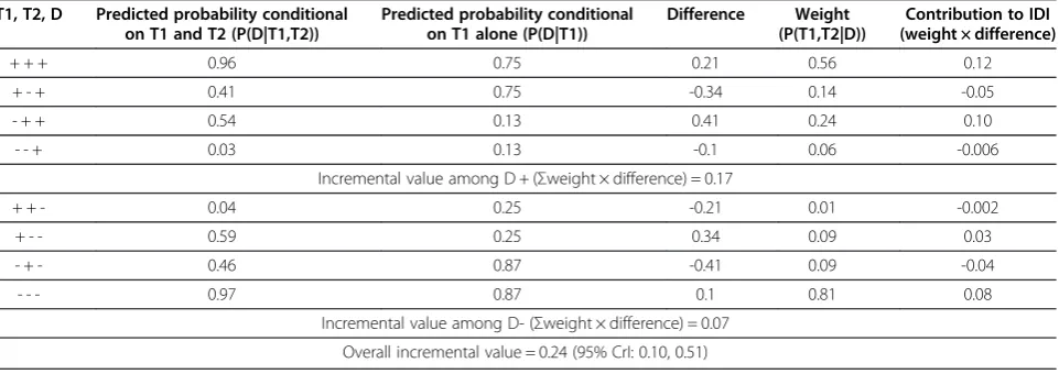
Table 1 illustrates the calculation of the IDI for the ex-pected dataset (i.e., the dataset obtained by multiplying the probabilities in (1) by the sample size of 1000) for the case when sensitivity of T2 was higher than that of T1. The IDI can be decomposed into the incremental value among true-positive and true-negative patients. In this scenario, the predicted probability given both T1and T2 increased among an estimated 17% of true-positive and 7% of true-negative patients, compared to the probability based on T1alone. Thus, the overall estimate of the IDI was 24%.
Table 1 Step-by-step calculation of Integrated Discrimination Improvement (IDI) when Test 2 (T2) has higher sensitivity than Test 1 (T1)*
T1, T2, D Predicted probability conditional on T1 and T2 (P(D|T1,T2))
Predicted probability conditional on T1 alone (P(D|T1))
Difference Weight
(P(T1,T2|D))
Contribution to IDI (weight × difference)
+ + + 0.96 0.75 0.21 0.56 0.12
+ - + 0.41 0.75 -0.34 0.14 -0.05
- + + 0.54 0.13 0.41 0.24 0.10
- - + 0.03 0.13 -0.1 0.06 -0.006
Incremental value among D + (Σweight × difference) = 0.17
+ + - 0.04 0.25 -0.21 0.01 -0.002
+ - - 0.59 0.25 0.34 0.09 0.03
- + - 0.46 0.87 -0.41 0.09 -0.04
- - - 0.97 0.87 0.1 0.81 0.08
Incremental value among D- (Σweight × difference) = 0.07
Overall incremental value = 0.24 (95% CrI: 0.10, 0.51)
D= disease status.
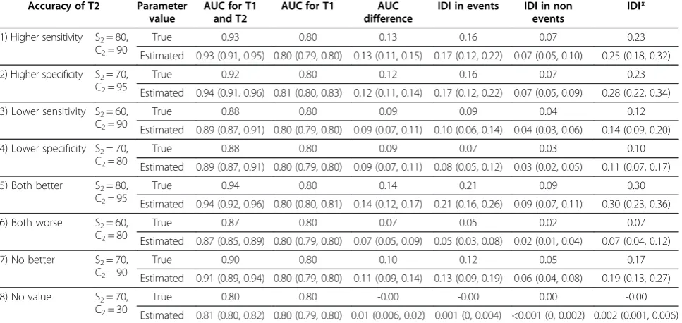
The true values of the AUCdiffand IDI for all simulation scenarios are shown in Table 2 together with the estimated posterior median values (median, 2.5% and 97.5% quan-tiles) across 1000 datasets. The true incremental value was greatest when both sensitivity and specificity of T2were higher than T1. As expected, the AUCdiff and IDI were close to 0 when T2had no value, such thatsens2+spec2= 0.7 + 0.3 = 1 (i.e., T2was no better than a coin toss). Even when both sensitivity and specificity of T2were lower than T1, there was some incremental value for T2. The incre-mental value was intermediate when either sensitivity or specificity of T2was better or worse than T1. In all scenar-ios, the estimated values of the incremental value statistics were very close to the true values across the 1000 datasets. The frequentist properties of the IDI and AUCdiffstatistics for each simulation scenario are given in Additional file 3: Table S3. In all scenarios, we find that the average cover-age (i.e., the estimated probability that the posterior 95% credible interval for a certain statistic included its true value) exceeds 95% and the average bias (i.e., the differ-ence between the true value and the posterior median) is low. We also confirmed convergence of the Gibbs sampler in each case (data not shown).
When T2had higher sensitivity and specificity than T1 (S2= 0.8, C2= .95), the true AUCdiff was 0.14, which was only slightly better than when T2had either higher sensi-tivity or higher specificity. In comparison, the magnitude
of the true IDI was larger (IDI = 0.30) when T2 had
higher sensitivity and specificity, compared to when T2 had either higher sensitivity (IDI = 0.25) or better specifi-city (IDI = 0.28). The IDI was lower when T2had lower specificity of 0.8 (IDI = 0.11) compared to lower sensi-tivity of 0.6 (IDI = 0.14), due to the prevalence being less than 50%.
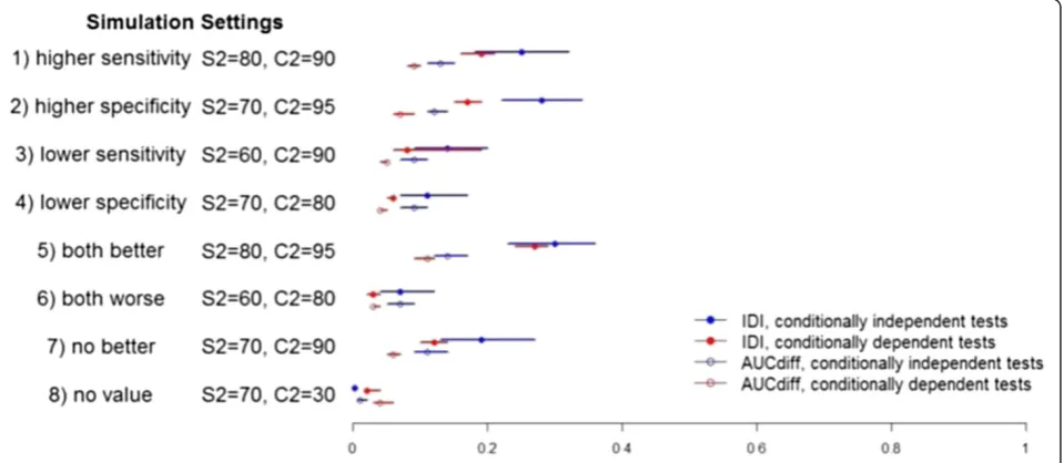
Impact of adjusting for conditional dependence
Table 3 shows the results for the simulations involving conditionally dependent tests: true values as well as a summary of the estimated values across 1000 simulated
datasets. The incremental value was largest when T2
had better sensitivity and specificity than T1and
smal-lest when T2was worse on both measures. When
com-paring this model to the one without adjustment for
conditional dependence, the incremental value of T2
was generally lower (Figure 1; Tables 2 vs 3). Interestingly, the true value of both incremental value statistics
sug-gested a small incremental value even when T2was not
useful: AUC = 0.04 and IDI = 0.02. This finding could be explained in part by the contribution of T2being positively correlated with T1. Once again, the average bias was very small and the average coverage exceeded 95% across the 1000 simulated datasets in each scenario (Additional file 4: Table S4).
Table 2 True values and posterior estimates across 1000 simulated datasets of Area Under the Curve (AUC) and Integrated Discrimination Improvement (IDI) statistics obtained from latent class models assuming conditional independence (with S1=0.7, C1=0.9)
Accuracy of T2 Parameter
value
AUC for T1 and T2
AUC for T1 AUC
difference
IDI in events IDI in non events
IDI*
1) Higher sensitivity S2= 80, C2= 90
True 0.93 0.80 0.13 0.16 0.07 0.23
Estimated 0.93 (0.91, 0.95) 0.80 (0.79, 0.80) 0.13 (0.11, 0.15) 0.17 (0.12, 0.22) 0.07 (0.05, 0.10) 0.25 (0.18, 0.32)
2) Higher specificity S2= 70, C2= 95
True 0.92 0.80 0.12 0.16 0.07 0.23
Estimated 0.94 (0.91. 0.96) 0.81 (0.80, 0.83) 0.12 (0.11, 0.14) 0.17 (0.12, 0.22) 0.07 (0.05, 0.09) 0.28 (0.22, 0.34)
3) Lower sensitivity S2= 60, C2= 90
True 0.88 0.80 0.09 0.09 0.04 0.12
Estimated 0.89 (0.87, 0.91) 0.80 (0.79, 0.80) 0.09 (0.07, 0.11) 0.10 (0.06, 0.14) 0.04 (0.03, 0.06) 0.14 (0.09, 0.20)
4) Lower specificity S2= 70, C2= 80
True 0.88 0.80 0.09 0.07 0.03 0.10
Estimated 0.89 (0.87, 0.91) 0.80 (0.79, 0.80) 0.09 (0.07, 0.11) 0.08 (0.05, 0.12) 0.03 (0.02, 0.05) 0.11 (0.07, 0.17)
5) Both better S2= 80, C2= 95
True 0.94 0.80 0.14 0.21 0.09 0.30
Estimated 0.94 (0.92, 0.96) 0.80 (0.80, 0.81) 0.14 (0.12, 0.17) 0.21 (0.16, 0.26) 0.09 (0.07, 0.11) 0.30 (0.23, 0.36)
6) Both worse S2= 60, C2= 80
True 0.87 0.80 0.07 0.05 0.02 0.07
Estimated 0.87 (0.85, 0.89) 0.80 (0.79, 0.80) 0.07 (0.05, 0.09) 0.05 (0.03, 0.08) 0.02 (0.01, 0.04) 0.07 (0.04, 0.12)
7) No better S2= 70, C2= 90
True 0.90 0.80 0.10 0.12 0.05 0.17
Estimated 0.91 (0.89, 0.94) 0.80 (0.79, 0.80) 0.11 (0.09, 0.14) 0.13 (0.09, 0.19) 0.06 (0.04, 0.08) 0.19 (0.13, 0.27)
8) No value S2= 70,
C2= 30
True 0.80 0.80 -0.00 -0.00 0.00 -0.00
Estimated 0.81 (0.80, 0.82) 0.80 (0.79, 0.80) 0.01 (0.006, 0.02) 0.001 (0, 0.004) <0.001 (0, 0.002) 0.002 (0.001, 0.006)
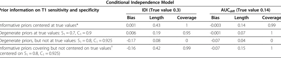
Sensitivity analysis in simulated scenarios
From Table 4 we can see that informative priors for S1 and C1that are centered on the true value of a parameter would lead to the lowest bias and highest coverage, even compared to the case when the parameters are fixed at the true values. When S1and C1are fixed at values that are incorrect, though not far from the true values, the bias in-creases and coverage dein-creases sharply to 0. On the other
hand, a wider prior that covers the true values but is not centered on them may have high coverage even though the bias is higher than the case when the prior is narrow and centered on the true values.
It has been reported that ignoring conditional depend-ence between the tests when it exists will result in the la-tent class analysis providing biased estimates of the sensitivity, specificity and prevalence of both tests [21,22]. Table 3 True values and posterior estimates across 1000 simulated datasets of Area Under the Curve (AUC) and Integrated Discrimination Improvement (IDI) statistics obtained from latent class models assuming conditional dependence (with S1=0.7, C1=0.9)
Accuracy of T2 compared to T1
Parameter value
AUC for T1 and T2
AUC for T1 AUC
difference
IDI in events IDI in non events
IDI*
1) Higher sensitivity S2= 80, C2= 90
True 0.88 0.80 0.09 0.10 0.04 0.15
Estimated 0.90 (0.89, 0.90) 0.80 (0.80, 0.81) 0.09 (0.08, 0.10) 0.13 (0.11, 0.15) 0.06 (0.04, 0.07) 0.19 (0.16, 0.21)
2) Higher specificity S2= 70, C2= 95
True 0.87 0.80 0.07 0.10 0.04 0.15
Estimated 0.88 (0.87. 0.89) 0.80 (0.80, 0.81) 0.07 (0.06, 0.09) 0.12 (0.10, 0.14) 0.05 (0.04, 0.06) 0.17 (0.15, 0.19)
3) Lower sensitivity S2= 60, C2= 90
True 0.84 0.80 0.04 0.03 0.01 0.04
Estimated 0.85 (0.84, 0.86) 0.80 (0.80, 0.81) 0.05 (0.04, 0.05) 0.05 (0.04, 0.06) 0.02 (0.02, 0.03) 0.08 (0.06, 0.19)
4) Lower specificity S2= 70, C2= 80
True 0.83 0.80 0.03 0.02 0.01 0.03
Estimated 0.85 (0.84, 0.86) 0.80 (0.80, 0.81) 0.04 (0.04, 0.05) 0.04 (0.03, 0.04) 0.02 (0.01, 0.02) 0.06 (0.05, 0.06)
5) Both better S2= 80, C2= 95
True 0.90 0.80 0.11 0.17 0.07 0.24
Estimated 0.91 (0.90, 0.92) 0.80 (0.79, 0.81) 0.11 (0.09, 0.12) 0.19 (0.16, 0.21) 0.08 (0.07, 0.09) 0.27 (0.24, 0.29)
6) Both worse S2= 60, C2= 80
True 0.82 0.80 0.02 0.01 0.00 0.01
Estimated 0.84 (0.83, 0.84) 0.80 (0.80, 0.81) 0.03 (0.03, 0.04) 0.02 (0.02, 0.03) 0.01 (0.007, 0.01) 0.03 (0.02, 0.04)
7) No better S2= 70,
C2= 90
True 0.85 0.80 0.05 0.05 0.02 0.07
Estimated 0.86 (0.85, 0.87) 0.80 (0.80, 0.81) 0.06 (0.05, 0.07) 0.08 (0.07, 0.10) 0.04 (0.03, 0.04) 0.12 (0.10, 0.14)
8) No value S2= 70,
C2= 30
True 0.84 0.80 0.04 0.01 0.01 0.02
Estimated 0.84 (0.83, 0.86) 0.80 (0.79, 0.80) 0.04 (0.03, 0.06) 0.02 (0.01, 0.02) 0.01 (0.004, 0.01) 0.02 (0.02, 0.04)
T1= test 1;T2= test 2;S2= sensitivity ofT2; C2= specificity of T2. *IDI is sum of IDIeventsand IDInon-events.
To study how ignoring conditional dependence will affect the incremental value statistics, we used the simulated
datasets from the scenario where T2had both improved
sensitivity and specificity compared to T1 and the two tests are conditionally dependent. We found that incor-rectly assuming conditional independence between the tests would result in over-estimating the incremental value. As seen in Table 3, the true values for this situation are AUCdiff=0.11 and IDI = 0.24. When ignoring the con-ditional dependence, the posterior median estimates were much higher across the 1000 simulated datasets: median AUCdiff= 0.15 [2.5% and 97.5% quantiles (0.13, 0.16)] and median IDI = 0.41 [2.5% and 97.5% quantiles (0.39, 0.47)].
Evaluation of QFT for LTBI
In the 2 published studies for the diagnosis of LTBI, the cross-tabulations of the test results were: TST + QFT + = 226, TST + QFT- = 62, TST-QFT + = 72, TST-QFT- = 359 for the Indian study [26] and TST + QFT + = 371, TST + QFT- = 532, TST-QFT + = 26, TST-QFT- = 289 for the Portuguese study [28]. Thus, the proportion of TST + QFT- results was higher in the Portuguese data. The esti-mates from the latent class model with conditional de-pendence appear in Table 5. For the Indian data, the AUCdiffwas 0.08 (95% CrI: 0.06, 0.11), while the IDI was 0.23 (95% CrI: 0.16, 0.29). For the Portuguese data, these values were AUCdiff= 0.21 (95% CrI: 0.17, 0.25) and IDI = 0.40 (95% CrI: 0.29, 0.51). Thus, both AUCdiffand IDI indicated greater incremental value of the QFT in the Portuguese population where multiple BCG vaccinations compromise the TST specificity. In both studies, the IDI for events and nonevents are relatively equal, suggesting that the QFT changes the probabilities for individuals with and without LTBI to a similar extent.
Evaluating the sensitivity to the prior distribution
When using Uniform instead of Beta prior distributions, the results remain unchanged (data not shown). When using wider prior distributions, the posterior distributions for the sensitivity were wider and the median estimates of the specificities of both tests were lower in both the Indian
and Portuguese data (Additional file 5: Table S5). Corres-pondingly, the median estimated incremental value statis-tics were all lower than those in Table 5. However, the credible intervals for these statistics (Additional file 5: Table S5) included the intervals in Table 5. Thus, our conclusion that the incremental value was higher for the Portuguese data remains unchanged.
Incremental value of QFT when using decision rules based on observed test results
In addition to the AUCdiff and IDI, the latent class
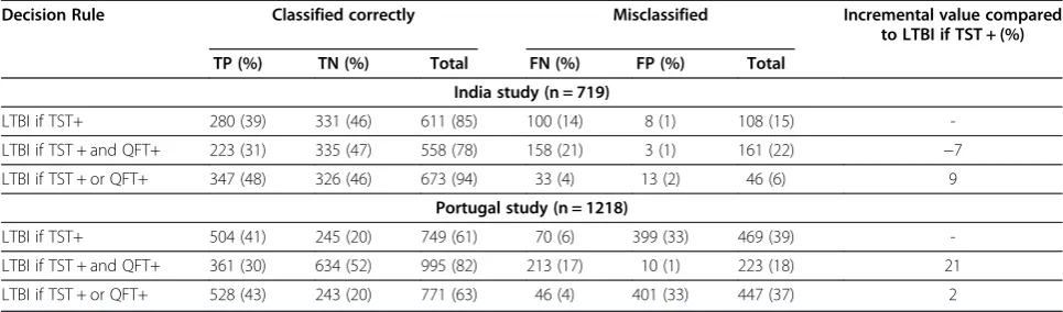
model can be used to determine the incremental value based on the observed TST and QFT results by estimat-ing the number of patients who are correctly classified as having or not having LTBI. As shown in Table 6, the TST + or QFT + decision rule would give the highest incremental value in the Indian data (9% increase in the number of correct diagnoses) mainly by increasing the proportion of true-positive patients compared to the diag-nosis based on TST alone. The TST + or QFT + decision rule, however, would be similar to using the TST alone in the Portuguese data. Instead, the TST + and QFT + deci-sion rule would result in the largest number of correctly-classified patients (21% increase in the number of correct diagnoses) mainly due to a decrease in the number of LTBI- patients who are false-positive. The difference in the preferred decision rule for the Indian and Portuguese data can be attributed to the different specificity of the TST test in these two groups. Nonetheless, the QFT test has incremental value over the TST in both populations. By calculating the incremental value as described, we can quantify precisely the expected impact of the differ-ence in specificity for the two groups.
Discussion
We have described how latent class models can provide information on the incremental value of a new diagnostic or screening test even in the absence of a gold standard
test. Our simulations show that both the AUCdiff and
IDI statistics can provide useful information on the Table 4 Sensitivity to prior distribution for the case when both sensitivity and specificity of the second test are better than the first test (true values are S1= 0.7, C1= 0.9)
Conditional Independence Model
Prior information on T1 sensitivity and specificity IDI (True value 0.3) AUCdiff(True value 0.14)
Bias Length Coverage Bias Length Coverage
Informative priors centered at true values* 0.001 0.43 1 -0.003 0.14 0.99
Degenerate priors at true values: S1= 0.7, C1= 0.9 0.006 0.19 0.95 -0.001 0.07 1
Degenerate priors, but not at true values: S1= 0.8, C1= 0.925 -0.17 0.08 0 -0.07 0.04 0
Informative priors covering but not centered on true values† (centered on S1= 0.8, C1= 0.925)
-0.16 0.42 0.99 -0.07 0.15 1
*S1 ~ Beta(58.1, 24.9) (95% CrI 0.6, 0.8), C1 ~ Beta(128.7, 14.3) (95% CrI 0.85, 0.95).
incremental value in the absence of a gold standard. As in the case when a gold standard is present, the IDI stat-istic has a larger relative magnitude compared to the AUCdiffand can be interpreted as the average improve-ment in the predictive value. By considering different simulation settings for the new test’s accuracy, we found that the incremental value was greatest when both sen-sitivity and specificity of a new test were better than the standard test and that both incremental value statistics were close to zero when the new test was of no value. When adjusting for conditional dependence between tests,
the incremental value of T2was lower. When the model
was mis-specified and ignored conditional dependence between the tests, both incremental value statistics were over-estimated as expected.
Bayesian estimation is particularly useful for latent class models that are non-identifiable due to insufficient degrees of freedom in the data, since it allows for the use of information external to the observed data. In our models, we used informative priors on the sensitivity and specificity of the standard test. As was the case in our motivating example of LTBI, evidence on these parameters can be obtained from the literature. One criticism of the latent class models we have used is their sensitivity to
prior information. We believe that we have used the best available information on sensitivity and specificity of the TST and QFT tests resulting from a meta-analysis. Further, we carried out sensitivity analyses to other prior distributions. As we have shown, the Bayesian ap-proach also provides credible intervals that have good coverage properties, unlike the limitations of the ap-proximate frequentist intervals described previously for the IDI statistic [30].
We have argued that in the absence of a gold standard, all available test results are needed in the latent class model to provide the best estimate of the true disease status. Indeed, clinicians almost always rely on all available clinical information to make diagnostic decisions [24]. Alternative approaches to latent class analysis, including use of a composite reference standard or panel diagno-sis, define a decision rule to definitively classify patients as disease positive or disease negative. Once such a defini-tive classification of disease status is obtained, methods for estimating incremental value in the presence of a gold standard may be used. The concern with this approach, of course, is that it may lead to reference standard bias [31]. In some situations, it may not be possible to implement these alternatives. In our motivating example, there were
Table 6 Median number of patients classified correctly or misclassified under each decision rule for diagnosis of Latent Tuberculosis Infection (LTBI)
Decision Rule Classified correctly Misclassified Incremental value compared
to LTBI if TST + (%)
TP (%) TN (%) Total FN (%) FP (%) Total
India study (n = 719)
LTBI if TST+ 280 (39) 331 (46) 611 (85) 100 (14) 8 (1) 108 (15)
-LTBI if TST + and QFT+ 223 (31) 335 (47) 558 (78) 158 (21) 3 (1) 161 (22) −7
LTBI if TST + or QFT+ 347 (48) 326 (46) 673 (94) 33 (4) 13 (2) 46 (6) 9
Portugal study (n = 1218)
LTBI if TST+ 504 (41) 245 (20) 749 (61) 70 (6) 399 (33) 469 (39)
-LTBI if TST + and QFT+ 361 (30) 634 (52) 995 (82) 213 (17) 10 (1) 223 (18) 21
LTBI if TST + or QFT+ 528 (43) 243 (20) 771 (63) 46 (4) 401 (33) 447 (37) 2
TP= true positive;FP= false positive;FN= false negative;TN= true negative.
Table 5 Median posterior estimates and 95% Credible Intervals (CrI) of latent class model parameters, Area Under the Curve (AUC) and Integrated Discrimination Improvement (IDI) statistics using data from applied examples
TST Sensitivity (95% CrI)
TST Specificity (95% CrI)
QFT Sensitivity (95% CrI)
QFT Specificity (95% CrI)
Prevalence (95% CrI)
India study (n = 719) [26]
0.74 (0.70, 0.78) 0.98 (0.96, 0.99) 0.76 (0.72, 0.80) 0.98 (0.96, 0.99) 0.53 (0.48, 0.58)
Portugal study (n = 1218) [28]
0.84 (0.81, 0.87) 0.46 (0.42, 0.51) 0.69 (0.62, 0.75) 0.98 (0.97, 0.99) 0.47 (0.41, 0.55)
AUC for TST and QFT (95% CrI)
AUC for TST (95% CrI)
AUC difference (95% CrI)
IDI in events (95% CrI)
IDI in non events (95% CrI)
IDI (95% CrI)
India study (n = 719) [26]
0.94 (0.91, 0.97) 0.86 (0.83, 0.89) 0.08 (0.06, 0.11) 0.11 (0.07, 0.14) 0.12 (0.08, 0.16) 0.23 (0.16, 0.29)
Portugal study (n = 1218) [28]
only two tests. Thus, it was not possible to define a composite reference standard. Moreover, if we used the simplistic approach of treating the older test as a gold standard, it would be equivalent to assuming that the new test has no incremental (or added) value. Hence, we feel a latent class approach is particularly valuable in this setting.
Since this is the first paper on the topic of estimating incremental value in the absence of a gold standard, we chose to focus on illustrating the concept in the simplest case involving only observed data from two diagnostic tests. We recognize that our model does not include pa-tient characteristics (e.g., age) that may play a role in the diagnostic decision-making process, thereby limiting the variation in predicted probabilities. Further research is needed to extend latent class models to incorporate such covariates that could have an effect on the prevalence, sensitivity or specificity [32]. In addition, more complex models can be used when test results are continuous or there are more than 2 tests involved. Findings from pre-vious work showing that increased sample size and an increase in informativeness of the prior distributions improve the precision of parameter estimates from a non-identifiable latent class model would also apply here [33], as all incremental statistics that we have described are functions of the prevalence, sensitivity and specificity parameters in the latent class model. In addition, more research is needed to examine the impact of the choice of a particular conditional dependence structure and the degree of conditional dependence on estimates of incre-mental value.
Another future direction would be estimating the more common NRI using plausible risk thresholds or even the category-free version [12]. In particular, our method may be able to address a recent criticism that the NRI cannot measure improvements in risk prediction at the popula-tion level [34], since the latent class model incorporates prevalence into the estimates. It should be mentioned that a number of recent articles have been critical of the IDI and NRI statistics [30,35]. In particular, it has been pointed out that they can be inflated for miscalibrated prediction models whereas the AUC may not be. This remains to be studied in the context when there is no gold standard.
An alternative approach to adding covariates to the model is to carry out a subgroup analysis. In our LTBI example, we estimated incremental value within sub-groups defined by study setting. The QFT had different incremental value beyond the TST depending on the population and BCG vaccination policy. In low-risk groups, using the TST + and QFT + decision rule could help avoid unnecessary LTBI therapy. On the other hand, using the TST + or QFT + decision rule could help clinicians who are worried about missing LTBI cases in high-risk groups, such as HIV/AIDS patients and young
children. Such reasoning has been used to support cost-effectiveness analyses of the TST and QFT for diagnosis of LTBI [36]. The Bayesian approach we propose is an improvement over such approaches since it takes into account the joint uncertainty in the sensitivity and speci-ficity parameters of both tests [37].
Several national guidelines now exist on using IGRAs such as the QFT, and many low-incidence countries rec-ommend a two-step process: if TST is positive then per-form the QFT as a confirmatory test [29]. This approach is equivalent to the“diagnose LTBI if TST + and QFT+” rule in terms of incremental value but is cheaper since not all patients receive both tests. In fact, the “diagnose LTBI if QFT+”rule (data not shown) would give similar results compared to the TST + and QFT + rule in the Portuguese data. However, the QFT is sold as a commer-cial kit that is more expensive than the TST. Ultimately, the decision to implement a new test into practice will depend on many factors, including patient preferences, risk of complications and cost considerations.
Conclusions
We have illustrated how to estimate incremental value in the absence of a gold standard test by relying on prior information on the sensitivity and specificity of one or both tests. Using point priors rather than prior ranges results in poor coverage and bias compared to using a wide prior, even if it is not centered on the true values. Further research is needed to develop methods for esti-mation of incremental value conditional on more tests and covariates.
Additional files
Additional file 1: Table S1.WinBUGS program for estimating the latent class model, IDI and AUCdiffstatistics.
Additional file 2: Table S2.Priors for T2 in simulation study of the conditional dependence model.
Additional file 3: Table S3.Average coverage, average bias and average length of 95% posterior credible intervals of AUCdiffand IDI
statistics resulting from fitting conditional independence latent class model to 1000 simulated datasets.
Additional file 4: Table S4.Average coverage, average bias and average length of 95% posterior credible intervals of AUCdiffand IDI
statistics resulting from fitting conditional dependence latent class model to 1000 simulated datasets.
Additional file 5: Table S5.Median posterior estimates and 95% credible intervals of parameters for latent class model and AUCdiffand IDI
statistics using data from applied examples when using wider prior distributions.
Competing interests
The authors declare that they have no competing interests.
Author’s contributions
of the results. ND designed the study, participated in the analysis and supervised the study. All authors read and approved the final manuscript.
Sources of funding
Financial support for this study was provided in part by the Canadian Institutes of Health Research (grants MOP-89857 and MOP-89918). DL is funded by a doctoral research studentship from the Canadian Thoracic Society. MP and ND are recipients of Chercheur Boursier salary awards from the Fonds de recherche Québec-Santé. The funding agreement ensured the authors’independence in designing the study, interpreting the data, writing, and publishing the report.
Received: 26 November 2013 Accepted: 8 May 2014 Published: 15 May 2014
References
1. Moons KG, Biesheuvel CJ, Grobbee DE:Test research versus diagnostic research.Clin Chem2004,50(3):473–476.
2. Moons KG, Van Es GA, Michel BC, Buller HR, Habbema JD, Grobbee DE: Redundancy of single diagnostic test evaluation.Epidemiology1999, 10(3):276–281.
3. Schunemann HJ, Oxman AD, Brozek J, Glasziou P, Jaeschke R, Vist GE, Williams JW Jr, Kunz R, Craig J, Montori VM, Bossuyt P, Guyatt GH, GRADE Workig Group:Grading quality of evidence and strength of
recommendations for diagnostic tests and strategies.BMJ2008, 336(7653):1106–1110.
4. Steyerberg EW, Vickers AJ, Cook NR, Gerds T, Gonen M, Obuchowski N, Pencina MJ, Kattan MW:Assessing the performance of prediction models: a framework for traditional and novel measures.Epidemiology2010, 21(1):128–138.
5. Hanley JA, McNeil BJ:The meaning and use of the area under a receiver operating characteristic (ROC) curve.Radiology1982,143(1):29–36. 6. Pepe MS, Janes H, Longton G, Leisenring W, Newcomb P:Limitations of
the odds ratio in gauging the performance of a diagnostic, prognostic, or screening marker.Am J Epidemiol2004,159(9):882–890.
7. Pencina MJ, D’Agostino RB Sr, D’Agostino RB Jr, Vasan RS:Evaluating the added predictive ability of a new marker: from area under the ROC curve to reclassification and beyond.Stat Med2008,27(2):157–172. discussion 207–212.
8. Pepe MS, Feng Z, Gu JW:Comments on‘evaluating the added predictive ability of a new marker: from area under the ROC curve to
reclassification and beyond’by M J Pencina et al.Stat Med2008, 27(2):173–181.
9. Reitsma JB, Rutjes AW, Khan KS, Coomarasamy A, Bossuyt PM:A review of solutions for diagnostic accuracy studies with an imperfect or missing reference standard.J Clin Epidemiol2009,62(8):797–806.
10. Joseph L, Gyorkos TW, Coupal L:Bayesian estimation of disease prevalence and the parameters of diagnostic tests in the absence of a gold standard.Am J Epidemiol1995,141(3):263–272.
11. Dendukuri N, Wang L, Hadgu A:Evaluating diagnostic tests forChlamydia trachomatisin the absence of a gold standard: a comparison of three statistical methods.Stat Biopharm Res2011,3(2):385–397.
12. Pencina MJ, D’Agostino RB Sr, Steyerberg EW:Extensions of net reclassification improvement calculations to measure usefulness of new biomarkers.Stat Med2011,30(1):11–21.
13. Dye C, Scheele S, Dolin P, Pathania V, Raviglione MC:Consensus statement. global burden of tuberculosis: estimated incidence, prevalence, and mortality by country. WHO Global surveillance and monitoring project. JAMA1999,282(7):677–686.
14. Christopher DJ, Daley P, Armstrong L, James P, Gupta R, Premkumar B, Michael JS, Radha V, Zwerling A, Schiller I, Dendukuri N, Pai M:Tuberculosis infection among young nursing trainees in South India.PLoS One2010, 5(4):e10408.
15. Pai M, Dendukuri N, Wang L, Joshi R, Kalantri S, Rieder HL:Improving the estimation of tuberculosis infection prevalence using T-cell-based assay and mixture models.Int J Tuberc Lung Dis2008,12(8):895–902. 16. Menzies D, Pai M, Comstock G:Meta-analysis: new tests for the diagnosis
of latent tuberculosis infection: areas of uncertainty and recommendations for research.Ann Intern Med2007,146(5):340–354.
17. Pai M, Riley LW, Colford JM Jr:Interferon-gamma assays in the immunodiagnosis of tuberculosis: a systematic review.Lancet Infect Dis2004,4(12):761–776.
18. Pai M, Zwerling A, Menzies D:Systematic review: T-cell-based assays for the diagnosis of latent tuberculosis infection: an update.Ann Intern Med2008,149(3):177–184.
19. Hadgu A, Dendukuri N, Hilden J:Evaluation of nucleic acid amplification tests in the absence of a perfect gold-standard test: a review of the statistical and epidemiologic issues.Epidemiology2005,16(5):604–612. 20. Gelman A, Rubin D, Stern H:Bayesian Data Analysis.New York: Chapman
and Hall; 1995.
21. Dendukuri N, Joseph L:Bayesian approaches to modeling the conditional dependence between multiple diagnostic tests.Biometrics2001, 57(1):158–167.
22. Torrance-Rynard VL, Walter SD:Effects of dependent errors in the assessment of diagnostic test performance.Stat Med1997, 16(19):2157–2175.
23. Staquet M, Rozencweig M, Lee YJ, Muggia FM:Methodology for the assessment of new dichotomous diagnostic tests.J Chronic Dis1981, 34(12):599–610.
24. Novielli N, Sutton AJ, Cooper NJ:Meta-analysis of the accuracy of two diagnostic tests used in combination: application to the ddimer test and the wells score for the diagnosis of deep vein thrombosis.Value Health2013, 16(4):619–628.
25. Farhat M, Greenaway C, Pai M, Menzies D:False-positive tuberculin skin tests: what is the absolute effect of BCG and non-tuberculous mycobacteria?Int J Tuberc Lung Dis2006,10(11):1192–1204. 26. Pai M, Gokhale K, Joshi R, Dogra S, Kalantri S, Mendiratta DK, Narang P,
Daley CL, Granich RM, Mazurek GH, Reingold AL, Riley LW, Colford JM Jr: Mycobacterium tuberculosis infection in health care workers in rural India: comparison of a whole-blood interferon gamma assay with tuberculin skin testing.JAMA2005,293(22):2746–2755.
27. Zwerling A, Behr MA, Verma A, Brewer TF, Menzies D, Pai M:The BCG World Atlas: a database of global BCG vaccination policies and practices. PLoS Med2011,8(3):e1001012.
28. Torres Costa J, Sa R, Cardoso MJ, Silva R, Ferreira J, Ribeiro C, Miranda M, Placido JL, Nienhaus A:Tuberculosis screening in Portuguese healthcare workers using the tuberculin skin test and the interferon-gamma release assay.Eur Respir J2009,34(6):1423–1428.
29. Denkinger CM, Dheda K, Pai M:Guidelines on interferon-gamma release assays for tuberculosis infection: concordance, discordance or confusion? Clin Microbiol Infect2011,17(6):806–814.
30. Kerr KF, McClelland RL, Brown ER, Lumley T:Evaluating the incremental value of new biomarkers with integrated discrimination improvement. Am J Epidemiol2011,174(3):364–374.
31. Hadgu A, Dendukuri N, Wang L:Evaluation of screening tests for detecting Chlamydia trachomatis: bias associated with the patient-infected-status algorithm.Epidemiology2012,23(1):72–82.
32. Hadgu A, Qu Y:A biomedical application of latent class models with random effects.Appl Stat1998,47:603–616.
33. Dendukuri N, Rahme E, Belisle P, Joseph L:Bayesian sample size determination for prevalence and diagnostic test studies in the absence of a gold standard test.Biometrics2004,60(2):388–397.
34. Kerr KF, Wang Z, Janes H, McClelland RL, Psaty BM, Pepe MS: Net reclassification indices for evaluating risk prediction instruments: a critical review.Epidemiology2014,25(1):114–121.
35. Hilden J, Gerds TA:A note on the evaluation of novel biomarkers: do not rely on integrated discrimation improvement and net reclassification index.Stat Med2013. doi:10.1002/sim.5804.
36. Oxlade O, Schwartzman K, Menzies D:Interferon-gamma release assays and TB screening in high-income countries: a cost-effectiveness analysis. Int J Tuberc Lung Dis2007,11(1):16–26.
37. Spiegelhalter D, Abrams K, Myles J:Bayesian Approaches to Clinical Trials and Health Care Evaluation.New York: John Wiley and Sons Limited; 2004.
doi:10.1186/1471-2288-14-67