Available online at http://ijdea.srbiau.ac.ir
Int. J. Data Envelopment Analysis (ISSN 2345-458X)
Vol.4, No.4, Year 2016 Article ID IJDEA-00422, 8 pages Research Article
Finding Outlier DMUs in Data Envelopment
Analysis
M. Mirbolouki
*Department of Mathematics, Yadegar-e-Imam Khomeini (RAH) Shahre Rey Branch,
Islamic Azad University, Tehran, Iran.
Received June 8, 2016, Accepted September 19, 2106
Abstract
Data Envelopment Analysis (DEA) is a mathematical programming for evaluating efficiency of a set of Decision Making Units (DMUs). One of the problems in DEA, is distinguishing outlier DMUs which have a different behavior in contrast to the general prevailing behavior of the population. The important issue is that the outlier DMUs, which are caused by the incorrect way of collecting data or other unknown factors which can be social, political and etc. , can affect the efficiency of other DMUs. Thus, recognizing and excluding them from the population or reducing their effect and proportioning their status with the population can influence the improvement of total efficiency of population. Therefore, as a result, it prevented the incorrect deduction about the population. In this paper, it is assumed that the efficiency of population must have a unimodal symmetric distribution, and a method based on the skewness of efficiency and inefficiency presented. The important contribution of this method is that it can recognize all the outlier DMUs, in different layers.
Keywords: Data Envelopment Analysis, Outlier, Skewness Coefficient, Normal
Distribution.
* E-Mail: [email protected]
1080
1. Introduction
DEA is a non-parametric method for evaluating the relative efficiency of DMUs with multiple inputs and outputs.Charnes et al. [4] have introduced CCR model which is based on constant returns to scale and after that Banker et al. [2] have proposed the variable returns to scale version of CCR model which has then referred to as BBC model. In the past few years, DEA approach has gain enormous popularity in practice and efficiency assessmant. A key feature of DEA, inorder to determine the performance of a specific DMU, is that it relatively compares the achievement of a DMU under consideration with the remaining DMUs. Also, DEA categorizes DMUs in efficient and inefficient groups. The relative efficiency in DEA is acquired through a comparison process with the efficient frontier which is constructed by efficient DMUs. Therefore, the efficiency score of inefficient DMUs is under effects of efficient DMUs. One of the applicable problem in field of DEA is distinguishing outlier DMUs. Outlier DMUs have a different behavior in contrast to the general prevailing behavior of the population, which is caused by the incorrect way of collecting data or other unknown factors which can be social, political and etc. Efficient outliers can affect the efficiency score of other DMUs. Therefore because of unusual state of outliers, in presence of these DMUs, the majority of population will be distinguished inefficient with very low efficiency scores. This situation may cause incorrect judgment about population. For example, consider a set of bank branches of a town and a central branch. It is obvious that the central branch is supported by lots of governmental organizations and the efficiency score of this branch is different with town branches. While these branches
is being assessed, an analyst may distinguish them as being unqualified to work by comparing their performance with that of the central branch. Thus recognizing and excluding outliers from the population, or reducing their effect and proportioning their status with the population can influence the improvement of total efficiency of population.
An outlier of a data set first defined by Barnett and Lewise [3]. Some of outliers are resultant from unusual characteristics which include uncontrollable factors, or factors which are in relation with the external environment. Even more, they are the resultants of measuring errors or observations pertaining to the low probabilities of occurrence. Also, Several approaches to detecting outliers in DEA have been described. Based on the "leave-one-out" idea Wilson [12] has addressed the presence of outliers and introduced a procedure for detecting them. He has verified that when a particular DMU is removed from the group, other DMUs can be affected. That is, based on the change in supper efficiency scores which is defined by Andersen and Petersen [1] the influence of outlier has been measured. Unfortunately, the Wilson's method [12] is computationally expensive and does not account for the frontier aspect of the problem. An influential observation typically owes its influence to the fact that it is an outlier and supports part of the deterministic frontier.
1081
attempt to detect outliers that are removed from the data cloud. Chen and Johnson [5] have proposed a unified model for detecting outliers by examining their effect on the boundaries of the convex hull constructed from a data set. Tran et al. [11] introduced another measure based on reference sets for detecting influential observations. In each of the influential measurement methods discussed previously in literature it has not been defined for which values of the obtained measure an outlier can be detected. In this paper assuming efficiency has a unimodal symmetric distribution a method based on the skewness of efficiency and inefficiency probability plots has been proposed. Also, the proposed method is not based on introducing an influential measurement. This method handles in detecting all efficient and inefficient outlier DMUs in different layers. The merit of this approach is its simplicity and applicability without defining influential measurements. The remainder of this paper is organized as follows: First DEA models for evaluating the efficiency and inefficiency are introduced. In section 3, with the contribution of skewness coefficient , an algorithm for finding outlier layers has been proposed. Section 4 conclude the paper.
2. Efficiency and inefficiency scores Let us assume n, homogenous DMUs consider observed output y j Rs 0
and input xj Rm 0 ,
x
j
0
,0
j
y for D M Uj , j = 1, 2,...,n. Each
j
D M U use
x
j to producey
j.Banker et al. [2] have proposed BBC model for evaluating the efficiency of DMUs. The production possibility set has been defined as follows:
=1
=1 =1
( , ) | ,
= , = 1,
0; = 1,...,
n
j j j
n n
B B C j j j
j j
j
x y x x
T y y
j n
The following is BCC model in input orientation for evaluating
DMU
o:*
=1
=1
=1
=
. . , = 1,...,
, = 1,...,
= 1
0, = 1,...,
o n
j ij io
j n
j rj ro j n j j j min
s t x x i m ,
y y r s ,
, j n
(1) * o
is the score of efficiency ofDMU
o and if
o*= 1;DMU
o is efficient, else if*
< 1
o
;DMU
o is inefficient.Jahanshahloo and Afzalinejad [8] have defined the full inefficient frontier. By the contribution of full inefficient frontier they also have proposed a model for identifying the worst score of efficiency.
j
DMU
is full inefficient if there is no other virtual DMU which is dominated byj
DMU
. That is,DMU
j is full inefficient if it belongs toF S
which is defined as follows:( , )| ( , ) (( , )
( ) =
( , ) ( , ) )
m s
x y x y R x y
F S S
x y x y S
1082
DMUs. Thus the full inefficient frontier in radial input orientation is defined as
I
F S where
( , ) | ( , ) & ( ) =
( > 1 ( , ) )
I
x y x y S
F S
x y S
Thus D M Uo is located on the full
inefficient frontier if in the following model we have
o*= 1, and it is not located on the full inefficient frontier if* *
=1 > 1 =
. , = 1 , ..., ,
o
o n
j ij io
j
m ax
s t . x x i m
=1 =1, = 1,..., ,
= 1,
0, = 1,...,
n
j rj ro j
n j j
j
y y r s
j n
(2)It should be noted that in model (2) *
1
o
and in model (1),
o*1. It is possible that while assessingDMU
o, models (1) and (2) results in
o* = 1 and*
= 1
o
; that is the DMU under assessment is located on both efficient and inefficient frontiers.Figure 1: Convex hull of DMUs with two input and one equal output.
In figure (1), the convex hull of DMUs is schematically portrayed. The piecewise linear frontier AGFE is the efficient frontier and ABCD is the inefficient frontiers. A is located on both efficient and inefficient frontiers, hence *
= 1
A and
A* = 1. H belongs to the interior of( )
F S thus *
> 1
H
and H* < 1. where
*
=
H
O L O H
and *
=
H
O K O H
.
3. Finding outlier layers with the contribution of skewness coefficient Normal frequency curve, is the most natural frequency curve which is symmetric and bell-shaped. In practice, there is no variable that its frequency
curve is completely normal. Usually the frequency curves of data are not symmetric. The extent to which the lack of symmetric-ness of frequency curve has been considered, is called skewness. The third central moment has been utilized inorder to calculate skewness. Let us assume that
r; = 1,...,
r
k
, be a set of data with
and S as mean and standard deviation, respectively. The average of; = 1,...,
r
r
k
, which is shown by 31083
Thus the skewness coefficient of data is computed from the following expression:
3 2
= m
Sk S
(3)
If data are symmetric as regards to the average, skewness coefficient equals zero and on basis of the sign of Sk , negative (positive) value, the frequency curve is respectively skewed to right (skewed to left). According to the Central Limit Theorem (see Hodges and Lehman [7]), in large sample size, every statistical distribution can be estimated with the normal distribution, If the distribution under assessment is symmetric, normal distribution of the estimation will be more reliable. Thus, in this paper instead of working with symmetric distribution under the guise of the suitable estimation, we prefer to work with normal distribution.
In this paper, with the expectation that the frequency curve of efficiency should be normal, we try to find the efficient and inefficient outlier layers. It should be noted that we expect that the efficiency in population has relative normal status and
a few of DMUs are efficient and a few of them are inefficient.
By applying model (1), the radial efficiency in input orientation can be found. If the frequency curve of
j's,= 1, 2,..., ,
j n is symmetric, it indicates that there is no outlier layer else, if the frequency curve is skewed to right or skewed to left, it results that there exists outliers DMUs.
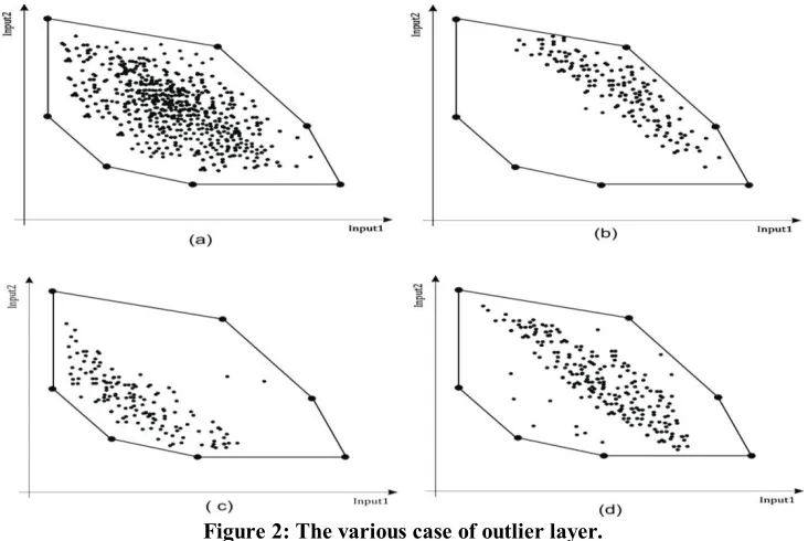
The estimation of efficient outlier layers or inefficient outlier layers, are the reasons why a frequency curve of efficiency cannot be symmetric. These cases are portrayed in figure (2) as follows:
Figure (2-a) indicates the situation in which there exists no efficient and inefficient outlier.
Figure (2-b) indicates the situation in which there exists few efficient outliers. In this case both of the frequency curve of
,
are skewed to right.Figure (2-c) indicates the situation in which there exists few inefficient outliers. In this case both of the frequency curve of
,
are skewed to left.1084
Figure (2-d) indicates the situation in which there exist both efficient and inefficient outliers. This case is the combination of cases (b) and (c) in which it is possible to have efficient outliers and by eliminating this layer and evaluating
the efficiency once more, inefficient outliers will be recognized. Note that the frequency curve of
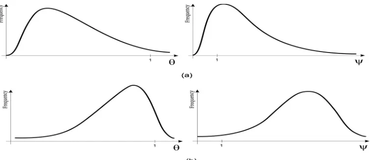
in this situation may have normal distribution which is similar to the case (a).Figure 3: Frequency curve of
,
for b and c cases of figure 2 respectively.In this paper the significant aim is to find all the efficient outlier layers since the DMUs which are located on this layer can affect the efficiency status of other DMUs. On the other hand DMUs which are located on the inefficient outlier layer have no affect on the efficiency status of other DMUs. It should be noted that detecting the inefficient outlier layers is important for recognizing whether the outlier layers have an effect on the skewness of the frequency curve of efficiency or not. The idea of this paper is based on computing the skewness coefficient of
j, = 1,...., ,
j
n
and,
= 1,...., .
j
j
n
If the skewness coefficient of
(Sk
) almost equals zero that is we accept that has normal distribution. Then we accept that there exists no efficient outlier. Otherwise considering
Sk
< 0
orSk
> 0
, we omit the efficient and inefficient layers, respectively. This procedures will be continued until theefficiency curve becomes symmetric. Below the algorithm of this procedure has been presented.
The algorithm of detecting outlier layers:
Initial step Let p = 0 ,q = 0,
= {1,...., }
N n ,
E
0=
andI
0=
Step1. For all j N , compute
*j from model (1).Step2. Test the hypothesis "the frequency curve of
is symmetric" versus rejection it. If this hypothesis is rejected, go to step 3 otherwise go to step 6.Step3. Compute
Sk
from the expression(3), if
Sk
< 0
go to step 4, else go to step 5.Step4. For all jN , compute
*j frommodel (2), let p =p 1 ,
* *
= { | = 1 & 1}
p
j j
I j N
,=
pN
N
I
and go to step 2.Step5. Let q =q 1,
N
=
N
E
q ,*
= { | = 1}
q
j
1085
Step6. Estimate
or standard deviation of
's for jN , if
= 1 belongs to6
interval, go to step 7, else go to step 5.Step7. End.
In the above algorithm, E 's and I 's indicate efficient and inefficient outlier layers respectively. After detecting outliers by rejecting the hypothesis of normality of
in step 2 and computingSk
, ifSk
< 0
then the algorithm identifies that there exists few inefficient outliers and removes them from the population. Note that a DMU on inefficient frontier may be located on the efficient frontier too, see point A in Figure (1), therefore algorithm does not remove efficient ones. Since removing any inefficient DMU does not affect on efficiency score of other DMUs, the hypothesis of step 2 need to be tested again. ifSk
> 0
, then the algorithm identifies that there exists few efficient outliers and removes them from the population, therefore due to this change in efficient frontier, the efficiency score must compute again. In step 6 by accepting normality of probability curve for
, algorithm examines wheatear= 1
belongs to 6
interval or not. Note that from statistical results, the interval of 6
, (3 , 3 ) , is the interval that 99% of data belong to it. Therefore if
= 1 does not belong to this interval, it results that there exist outliers or on the other hand algorithm identifies efficient outlier DMUs. Consider Figure (2) and the difference between Figure (2-a) and Figure (2-d).Finally efficient outlier layers
E E
1,
2,...
and inefficient outlier layersI I
1,
2,...
can be obtained with the contribution the mentioned algorithm. After that the efficient status becomes symmetric on basis of manager's decisions, DMUswhich are located on the efficient outlier layers can be excluded from the population. Also inputs and outputs of these DMUs can be got well-proportioned to the population status, that is their effects in population can be reduced. 4. Conclusion
1086
References
[1] Andersen, P., Petersen, N.C. A procedure for ranking efficient units in data envelopment analysis, Manage. Sci. V.39, N.10, 1993, pp.1261-1264.
[2] Banker, R.D., Charnes, A., Cooper, W.W. Some models for estimating technical and scale in efficiencies in data envelopment analysis, Manage. Sci. V.30, N.9, 1984, pp.1078-1092.
[3] Barnett, V., Lewise, T. Outlier in Statistical Data. John Wiley, New York, 1994.
[4] Charnes, A., Cooper, W.W., Rhodes, E. Measuring the efficiency of decision making units. Eur. J. Ope. Res. V.2, N.6, 1978, pp.429-444.
[5] Chen, W.C.,Johnson, A.L. A Unified Model for Detecting Efficient and Inefficient Outliers in Data Envelopment Analysis, Comput. Oper. Res. V.37, N.2, 2009, pp.417-425.
[6] Fox, K.J., Hill, R.J., Diewert, W.E. Identifying outliers in multi-output models, J. Prod. Anal. V.22, N.2, 2004, pp.73-94.
[7] Hodges, J.L., Lehmann, E.L. Basic Concepts of Probability and Statistics, Holden-Day, San Francisco, 1970.
[8] Jahanshahloo, G.R., Afzalinejad, M. A ranking method based on a full-inefficient frontier, Appl. Math. Model. V.30, N.3, 2006, pp.248-260.
[9] Pastor, J.T., Ruiz, J.L., Sirvent, I. A statistical test for detecting influential observations in DEA, Eur. J. Oper. Res. V.115, N.3, 1999, pp.542-54.
[10] Simar, L. Detecting Outliers in Frontier Models: A Simple Approach, J. Prod. Anal. V.20, N.3, 2003, pp.391-424. [11] Tran, N.A., Shively, G., Preckel, P. A new method for detecting outliers in Data Envelopment Analysis, Appl. Econ. Lett. V.17, N.4, 2010, pp.313-316. [12] Wilson, P.W. Detecting influential observations in data envelopment analysis, J. Prod. Anal. V.6, N.1, 1995, pp.27-45.