Deterministic walk on Poisson point process

DETERMINISTIC WALK ON POISSON POINT PROCESS

Simon Le Stum

Abstract. A deterministic walk on a Poisson point process inRd

is an oriented graph where each point of the process is connected to only one other point following a deterministic and stationary rule of connection. In the paper we investigate the absence of percolation for such graphs and our main result is based on two assumptions. The Loop assumption ensures that any forward branch of the graph merges on a loop provided that the Poisson point process is augmented with a finite collection of well-chosen points. The Shield assumption ensures that the graph is locally determined with possible random horizons. Among the models which satisfy these general assumptions and inherit in consequence the finite cluster property, we focus on the deterministic walk to thek-th neighbour, withk any integer greater than one.

Résumé. Une marche déterministe sur un processus ponctuel de Poisson de Rd _{consiste à} connecter chaque point du processus à un et un seul autre en suivant une règle déterministe invariante par translation. Dans ce papier, nous donnons un résultat général d’absence de composante connexe infinie pour de tels graphes dès que le modèle vérifie deux hypothèses. La première hypothèse, appelée hypothèse Loop, garantit que les branches descendantes du graphe finissent par boucler du moment qu’une collection bien choisie de points est ajoutée au processus initial. La seconde, appelée hypothèse Shield, assure que le graphe est déterminé localement avec éventuellement un horizon de détermination aléatoire. Parmi tous les modèles satisfaisant ces deux hypothèses nous nous intéressons tout particulièrement à la marche déterministe au k-ième plus proche voisin, aveckun entier plus grand que un.

Introduction

The classical nearest neighbour walk based on a planar homogeneous Poisson point process consists in connecting each point to its nearest neighbour. The absence of infinite cluster for this model is due to the fact that almost surely a homogeneous Poisson point process does not have a descending chain. By a descending chain, we mean an infinite sequencex1, x2, ...of points of the process for which |xi−1−xi| ≥ |xi−xi+1|for alli≥2. Letkbe an integer larger than 2, is there an infinite cluster if each

vertex of a Poisson point process is connected to its k-th nearest neighbour? It is easy to notice that the descending chain argument is not available in this setting and that the graph is more complicated and strongly interlaced, especially whenkis large. If, instead of connect each vertices to itsk-th nearest neighbour, the vertex is connected randomly and uniformly among its first k neighbours, the absence of percolation could also be obtained with a descending chain argument. Indeed the uniform random choice ensures that, with positive probability, the son and the father of a vertex are the same. So there is an infinite number of opportunities for producing a loop and therefore the loop exists with probability one. Obviously each opportunity is possible provided that the father of the vertex belongs to its firstk

neighbours, which is related to a descending chain argument: roughly speaking, along each possible infinite branch, it appear long descending chains. When the choice among thekneighbours is deterministic (as,

1_{Laboratoire Paul Painlevé Université Lille 1}

© EDP Sciences, SMAI 2017

for instance, in the deterministic walk to thek-th neighbour) the problem is more complicated since the creation of a loop is more difficult. As far as we know, there does not exist a proof of the absence of percolation for the deterministick-th nearest neighbour walk by using a descending chain argument.

In this paper, the absence of percolation for the k-th nearest neighbour walk in Rd is obtained as a consequence of our main result (Theorem 1.1). This result is a simplified version of Theorem 3.1 in [2] where the connection rule is possibly random. In our main theorem we consider general oriented outdegree-one graphs based on the vertices of a stationary Poisson point process. Since the graph is oriented, we can define the Forward and Backward sets of any given vertexx: see Section 1.2 for a precise definition. Then, the cluster containing x merely is the union of these both sets. The outdegree-one structure implies that any forward branch is finite if and only if it contains a loop. A loop is defined as a finite sequencex1, x2, . . . , xn of different vertices such thatxi is connected toxi+1 for 1≤i≤n−1 and

xn is connected tox1. A general argument for stationary outdregree-one graphs, called mass transport

principle, and mentioned for example in [4] and [2], ensures that the absence of forward percolation implies the absence of backward percolation. On the oriented outdegree-one Poisson graph the aim of the work is to provide general assumptions ensuring that any forward branch of Poisson outdegree-one graphs merges on a loop.

The proof of our main theorem, given in [2] is based on a general statement for Poisson outdegree-one graphs which can be interpreted as a counterpart of the mass transport principle: roughly speaking, if there exists, with positive probability, an infinite forward branch then the expectation of the size of a typical backward branch is infinite. An important part of the work in [2] was to exhibit two assumptions which guarantee that such expectation is finite. Let us describe briefly these assumptions. The first one, called the Loop assumption, assumes that any forward branch merges to a loop if the process is augmented with a finite collection of well-chosen points (without reducing the size of the backward). This assumption ensures that a loop is possible along a forward branch provided that some points are added. In general this fact is obvious for all models for which the loops are possible. The extra condition on the size of the backward is directly related to the method we use. The second one, called the Shield assumption, is directly inspired from the ones done by Hirsch, see Section 3 of [4]). More or less, it assumes that with high probability, the graph contains no edge crossing large boxes. In this paper we show in particular that thek-th nearest neighbour walk inRd satisfies these assumptions and therefore the absence of percolation occurs.

The paper is organized as follows. In Section 2, we provide a precise description of stationary deter-ministic walks built on a Poisson point process, illustrated by the example of thek-th nearest neighbour walk inRd. We achieve this section by describing our both assumptions and the main result (Theorem 1.1) ensuring the absence of percolation. Section 3 is devoted to check that the k-th nearest neighbour walk inRd satisfies the assumptions of Theorem 1.1. Finally, in Section 4, we give a sketch of proof of Theorem 1.1.

1.

Results

In this section, we give another version of Theorem 3.1 of [2] adapted to the deterministic walks on Poisson environment.

1.1.

_Notations

In this paper, all geometric models take place in the Euclidean spaceRd. The configuration spaceC

onRd is defined as

C ₌n_ϕ⊂Rd_{;NΛ(ϕ)<∞, for any bounded Λ⊂R}do

whereNΛ(ϕ) = #ϕΛ denotes the number of points ofϕwhich lie in Λ (for a given subset Λ of Rd, and

ϕ∈C_{,ϕΛ denotes the set of points ofϕincluded in Λ: ϕΛ=ϕ∩Λ).}

As usual, the configuration spaceC _{is equipped with theσ-algebra}

generated by the counting eventsP(A,n)={ϕ∈C; NΛ(ϕ)≤n}. Similarly, for any subset Λ⊂Rd, we

define theσ-algebra of events in Λ by

S_{Λ=σP(A,n);A⊂Λ, n≥0.}

Letv ∈Rd. The translation operator τv acts onRd and C as follows: for any x∈Rd andϕ∈C, we

set τv(x) = v+x and τv(ϕ) = ∪x∈ϕ{τv(x)}. Finally, a subsetC′ ⊂C is said translation invariant if

τv(C′) =C′, for any vectorv∈Rd.

1.2.

_{The outdegree-one model}

In our setting, anoutdegree-one graphis an oriented graph whose vertex set is given by a configuration

ϕ∈C _{and has exactly one outgoing edge per vertex. Such graph can be described by agraph function}

which determines, for any vertex, its outgoing neighbour.

Definition 1.1. Let C′ _⊂C _{be a translation invariant set. A functionh from}C′_×Rd _toRd _{is called} agraph functionif:

(i) ∀ϕ∈C′_{,∀x∈ϕ, h(ϕ, x)∈ϕ\{x};}

(ii) ∀v∈Rd,∀ϕ∈C′_{,∀x∈ϕ, h(τv(ϕ), τv(x)) =τv(h(ϕ, x)).} The couple(C′_{, h)is then called anoutdegree-one model.}

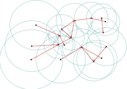
In the sequel, we consider an outdegree-one model (C′_{, h) and a configuration ϕ∈}C′_{. The oriented}

graph is made up of edges (x, h(ϕ, x)), for all x∈ϕ. Like Figure 1 shows, this graph is not necessarily planar.

Let us describe the structure of the clusters. Letx∈ϕ. TheForward set For(x, ϕ) ofxinϕis defined as the sequence of the outgoing neighbours starting atx:

For(x, ϕ) ={x, h(ϕ, x), h(ϕ, h(ϕ, x)), . . .} .

The outdegree-one property ensures that the Forward set is finite if and only if it contains a loop, i.e. a subset {y1, . . . , yl} ⊂ For(x, ϕ), with l ≥ 2, such that for any 1≤ i ≤ l, h(ϕ, yi) = yi+1 (where the

indexi+ 1 is taken modulol). In this case, the integerl is called thesizeof the loop. TheBackward set

Back(x, ϕ) ofxin ϕcontains all the vertices y∈ϕhavingxin their Forward set:

Back(x, ϕ) ={y∈ϕ;x∈For(y, ϕ)}.

The Backward set Back(x, ϕ) admits a tree structure whosexis the root. The Forward and Backward sets ofxmay overlap; they (at least) containx. Their union forms theCluster ofxinϕ:

C(x, ϕ) = For(x, ϕ)∪Back(x, ϕ).

Our main theorem (Theorem 1.1) states that for a large class of random models, all the clusters are a.s. finite. Furthermore, the outdegree-one property implies that there is at most one loop in a cluster. Hence, a finite cluster is made up of one loop with some finite trees rooted at vertices of the loop. Obviously, this notion of loops will be central in our study.

In the sequel, the configuration will be generated by a Poisson point process (PPP)Xwith intensity measure λd (the Lebesgue measure on Rd). This means that the random variable #(X∩A) follows

a Poisson distribution with parameter λd(A), for any bounded set A ⊂ Rd. By scaling, any other

(stationary) intensity measure of the formzλd withz >0 could be considered.

Finally, let us denote by (Ω,F_{,P) a probability space on which the PPP Xis defined.}

Definition 1.2. Let (C′_{, h)be an outdegree-one model. If P(X∈C}′_{) = 1 then the triplet (C}′_{, h,X) is}

called a random outdegree-one model.

1.3.

_The

k

_{-nearest neighbour walk in R}

Letk∈N∗ be an integer which will be the range of the walk. Givenx∈Rdandr >0,B(x, r) define the open Euclidiean ball of radius rand centred on x. Letϕ∈ C _{and x∈ϕ, we define the set of the}

k-nearest neighbour of xin ϕ:

Nk(ϕ, x) ={y∈ϕ; NB(x,kx−yk2)(ϕ) =k}.

Let us defineC′ _{as well,}

C′ _={ϕ∈C _{; ∀x∈ϕ, #Nk(ϕ, x) = 1}.}

For each ϕ ∈ C′ _{and each x ∈ ϕ, h(ϕ, x) corresponds to the only point of Nk(ϕ, x). Using standard}

properties of the PPP, it is easy to show thatXcontains no isosceles triangles a.s, and therefore (C′_{, h,X)} is a random outdegree-one model.

As mentioned in the introduction, for k ≥ 2, in a forward branch the length of the edges is not necessary decreasing .

x

Figure 1. _{In this picture, the dimensiondequals to 2 andk= 3. The oriented graph is}

drawn in red. We can see four clusters, three of them have a loop of size 2, the other one has a loop of size 3. The circles are drawn to help to recognize the 3-nearest neighbours of each point

Let us set others examples of deterministic walks on a Poisson point process. The hard sphere lilypond model built on a Poisson configuration introduced in [3] can be observed like a out-degree one graph. The authors prooved the absence of percolation for this model. We can also talk about the 2D-directed spanning forest, the authors of [1] prooved that this Poisson oriented graph is almost surely a tree (unicity of infinte cluster).

1.4.

_{Assumptions and Theorems}

We first establish in Theorem 1.1 the absence of percolation for all random outdegree-ones (C′_{, h,X)}

satisfying two general assumptions, namely theLoop and Shield assumptions, which are described and commented below. Thus, Theorem 1.2 asserts that thek-nearest neighbour walk verifies these two as-sumptions and therefore does not percolate.

Loop assumption

Letϕ∈C′ _{andl be a positive integer. The configurationϕ is said l-looping if for any x∈ϕ, there}

exists an open setAx⊂ {(x1, . . . , xl)∈Rdl ; ∀i=6 j, xi 6=xj} such that, for all (x1, . . . , xl)∈Ax:

(i) For(x, ϕ∪ {x1, . . . , xl})⊂ {x, x1, . . . , xl};

(ii) #Back(x, ϕ∪ {x1, . . . , xl})≥#Back(x, ϕ).

Given x, conditions (i) and (ii) can be interpreted as a local modification of the configurationϕ which breaks the Forward set ofxwithout altering its Backward set– or at least without decreasing the cardi-nality of its Backward set. Whereas condition (i) is very natural to obtain a finite cluster, condition (ii) is more technical and will appear in the proof of Proposition 4.3 in [2]. The choice of the integer l will be specific to the random outdegree-one graph (C′_{, h,X).}

We will say that the random outdegree-one graph (C′_{, h,X) satisfies the Loop assumption if there}

exists a positive integerl such that

P(X isl-looping ) = 1.

Shield assumption

Figure 2. _{To simplify the picture, we have chosenα=} 1

2 so thatAi= (Ai⊕[

−1 2 ;

1 2]d), ∀i = 1,2. The white points are the elements of mV while the black ones are those of

mA1(insidemV) andmA2(outsidemV). Red squares are points ofϕ. Ifτ−mz(ϕ)∈Em

for all z ∈ V, then it is impossible for a (red) segment [x;x′], where h(ϕ, x) = x′, to cross the setm(V ⊕[−α;α]d_{) frommA}

1 tomA2– or from mA2 to mA1 by symmetry

of Equation (2) w.r.t. indexes 1 and 2.

The Shield assumption is a kind of strong stabilizing property for the random outdegree-one graph (C′_{, h,X) and has been first introduced in a slightly different way in [4].}

We will say that the random outdegree-one graph (C′_{, h,X) satisfies the Shield assumption if there} exist a positive realαand a sequence of events (E_{m)m≥1 such that:}

(i) ∀m≥1,E_m∈S_[−αm;αm]d;

(ii) P(E_{m) −→}

m→∞1;

(iii) Consider the latticeZd with edges given by{{z, z′},|z−z′|∞= 1}and any three disjoint subsets

A1, A2, V ofZd such that∀i= 1,2, the boundary∂Ai ={z∈Zd\Ai,∃z′ ∈Ai,|z−z′|∞= 1}is included inV. Let us set

Ai=

Ai⊕ h−1

2 ; 1 2

id

Then, form sufficiently large and for any configurationsϕ, ϕ′ ∈C′ _{such that τ−mz(ϕ)∈}E_mfor

allz∈V, the following holds:

∀x∈ϕmA1, h(ϕ, x) =h(ϕmA

c

2∪ϕ

′

mA2, x). (2)

In Condition (iii), the setmV acts as an uncrossable obstacle, i.e. a shield between setsmA1 andmA2.

See Figure 2. Equation (2) says that the outgoing neighbour of anyx∈ϕmA1 does not depend on the configuration onmA2. In particular,h(ϕ, x)∈ϕmAc

2. Here are our main results.

Theorem 1.1. Any random outdegree-one graph(C′_{, h,X)satisfying the Loop and Shield assumptions}

does not percolate with probability1:

P(∀x∈X,#C(x,X)<∞) = 1.

Theorem 1.1 is proved in [2] in a more general context and a sketch of its proof is given in Section 3 of this paper.

Checking that the model given in Section 1.3 satisfies the Loop and Shield assumptions, we get:

Theorem 1.2. For each k∈N∗, thek-nearest neighbour walk inRd does not percolate with probability

1.

0 0.1 0.2 0.3 0.4 0.5 0.6 0.7 0.8 0.9 1 0

1

0.2 0.4 0.6 0.8

0.1 0.3 0.5 0.7 0.9

Figure 3. _{In this simulation, we draw, in a [0,1]}2_{, the 30-nearest neighbour walk}

starting to (1 2,

1

2). The intensity value is 500. We observe that the forward component

of (1₂,1₂) is finite.

Hence, we will see in Proposition 2.1 thatl points suffice to make a loop for the l-nearest neighbour walk.

2.

Proof of Theorem 1.2

Let us introduce some usual notations. For a given vertexx∈ϕ, we split the Euclidean ballB(x,kx−

h(ϕ, x)k2) intokdisjoint regions. By induction, fori∈Nwe definevi(ϕ, x) as follows;v0(ϕ, x) =x, and,

fori≥1 vi(ϕ, x) is the unique nearest neighbour ofxin the configurationϕ\ {v0(ϕ, x), . . . , vi−1(ϕ, x)}.

Precisely, fori≥1,vi(ϕ, x) is the uniqueithnearest neighbour ofxinϕ, in particular,h(ϕ, x) =vk(ϕ, x).

Thus we set, fori∈ {1, . . . , k},

C1(ϕ, x) = B(x,kx−v1(ϕ, x)k2),

∀i∈ {2, . . . , k}, Ci(ϕ, x) = B(x,kx−vi(ϕ, x)k2)\B(x,kx−vi−1(ϕ, x)k2).

Then, we obtain

B(x,kx−h(ϕ, x)k2) = [

1≤i≤k

Ci(ϕ, x).

2.1.

_{Loop assumption}

Thek-nearest neighbour walksatisfies the Loop assumption.

Proposition 2.1. Almost all configurations of C′ _{is k-looping.}

Proof:We prove that there existsC′′ _⊂C′_{such that any configuration of}C′′_{isk-looping andP[}C′′_{] = 1.}

For a given pointx∈ϕ, create a loop in the forward set ofxis relatively easy, it is sufficient to reduce the radius of the open ballC1(ϕ, x) and to put exactlykpoints inside. In the rest of the proof, we note by B(ϕ, x) the ballB(x,kx−v1(ϕ,x)k2

2 ). The difficulty is that nothing ensures that the size of the backward set

ofxis not reduced. Precisely, it could exist a pointy∈Back(ϕ, x) such thatB(y,ky−h(ϕ, y)k2) contains

at least one point among thek points added. In this new configuration, the kth_{-nearest neighbour ofy}

would be changed. Let us consider the set of points

E_{(x, ϕ) ={y∈ϕ\ {x} ; B(y,ky−h(ϕ, y)k2)∩B(ϕ, x)6=∅}.}

The main part of the proof consists in checking that if E_{(x, ϕ) is finite, then there exists an open set}

Ax which satisfies the two items of the Loop assumption. Then, the following subset of configurations is

introduced

C′′_={ϕ∈C′ _{; ∀x∈ϕ, #}E_{(x, ϕ)<∞}}

First, we check thatE[#E_{(0,X∪ {0})]<∞following the strategy described by the proof of Lemma 5.1}

in [2].

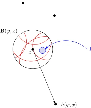
Now we have to show that all configurations inC′′ _{are k-looping. We fixϕ∈}C′′ _{andx∈ϕ. Since} E_{(x, ϕ) is finite, then there exists an open ball Γ such that, for ally∈}E_{(x, ϕ), and for alli∈ {1, . . . , k},}

Ci(ϕ, y)∩Γ6=∅ =⇒ Γ⊂Ci(ϕ, y). (3)

This implication is illustrated in Figure 4.

The diameter of Γ is chosen smaller than the distance betweenxand Γ to ensure that thekth-nearest neighbour of each point added is x. In other words, for all distinct points x1, . . . , xk ∈ Γ and for all

i∈ {1, . . . , k},h(ϕ∪ {x1, . . . , xk}, xi) =x.

Let us define the open set

Ax={(x1, x2, . . . , xk)∈Γk ; ∀i6=j, xi6=xj}.

Then, we can verify that for all (x1, . . . , xk)∈Ax,

(i) For(x, ϕ∪ {x1, . . . , xk})⊂ {x, x1, . . . , xk};

x

h(ϕ, x) B_{(ϕ, x)}

Γ

Figure 4. _{For eachy ∈}E_{(x, ϕ), the boundary ofCi(ϕ, y) is drawn in red. There is a}

finite number of red arc which overlapB(ϕ, x), that is why it is possible to insert a ball which is not overlapped by any arc.

The first item is obtained as a consequence of the two following facts; for (x1, . . . , xk)∈ Ax, h(ϕ∪ {x1, . . . , xk}, x)∈ {x1, . . . , xk}(becausexi∈C1(ϕ, x) for alli∈ {x1, . . . , xk}) and,h(ϕ∪{x1, . . . , xk}, xi) =

xfor anyi∈ {1, . . . , k}.

The second item is obtained as a consequence of (3): Let (x1, . . . , xk)∈Ax andy∈Back(ϕ, x)\ {x}.

There exist n ∈ N∗ _{and y}

0, . . . , yn ∈ ϕ such that; y0 = y, yn = x and yj+1 = h(ϕ, yj) for all j ∈ {0, . . . , n−1}. Two situations may occur:

• If, for allj ∈ {0, . . . , n−1}and for all i∈ {1, . . . , k}, Ci(ϕ, yj)∩B(ϕ, x) =∅ then, y is clearly

still in the backward set ofxsinceh(ϕ∪ {x1, . . . , xk}, yi) =yi+1 for anyi∈ {1, . . . , n−1}.

• Otherwise, we consider the first indexj0 ∈ {0, . . . , n−1} such that there exists i ∈ {1, . . . , k}

satisfying x1, . . . , xk ∈ Ci(ϕ, y). It implies that vk(ϕ∪ {x1, . . . , xk}, yj0) ∈ {x1, . . . , xk}, then,

h(ϕ∪ {x1, . . . , xk}, yj0) ∈ {x1, . . . , xk} and y is still in the backward set of x since h(ϕ∪ {x1, . . . , xk}, xi) =xfor anyi∈ {1, . . . , k}.

The Loop assumption is proved for this model.

2.2.

_{Shield assumption}

Let us split the hypercube [−m;m]d_{intoκ= (d⌊m}1/d_⌋)d_{congruent subcubesQ}m

1, . . . , Qmκ (⌊·⌋denotes

the integer part). Each of these subcubes has an area equal to

dm d⌊m1/d_⌋

d

,

i.e. of ordermd−1_{. Thus, we define the eventE}

mas follows:

E_m= \

1≤i≤κ

#XQm

i ≥k .

x

Figure 5. _{Black points are vertices mz for z ∈ V. The event} E_{m realized on each}

z⊕[−m;m]d _{provides a shield betweenmA}

1 andmA2. Indeed, a given ball centred on

xcannot overlapmA2 without containing a subsquarez+Qmi .

Proof: Let us first remark that the eventE_misS_[−m,m]d-measurable and its probability tends to 1. So

the first two items of the Shield assumption are satisfied withα= 1.

Let us focus on Item (iii). Hence, let us considerV, A1, A2⊂Zd such that the topological conditions

of the shield assumption occur. Let us consirerAi as defined in (1) fori∈ {1,2}. Letϕ∈C

′

satisfying

ϕ−mz∈E_{m, for any vertexz∈V. Letx∈ϕbe a point which belongs tomAi. It is sufficient to remark}

that for anym, any open ball centred onxwhich overlapsmAi contains at least one subsquarez+Qmi .

Hence, the outgoing vertexh(ϕ, x) remains unchanged.

3.

Sketch of the proof of Theorem 1.1

Theorem 1.1 is rigorously proved in [2]. Let us talk about the main steps and arguments of the proof. We have to prove that any random outdegree-one model which satisfies the Loop and Shield assump-tions, does not contain any infinite cluster with probability 1:

P ∀x∈X,#For(x,X)<∞ and #Back(x,X)<∞

= 1. (4)

First, thanks to a standard mass transport argument, we can reduce the proof of the absence of percolation to the absence of forward percolation. This argument is only implied by the stationarity of X and is proved in [4] and [2] :

P ∀x∈X,#For(x,X)<∞

= 1 =⇒ P ∀x∈X, #Back(x,X)<∞

= 1. (5)

Reasoning by contradiction, we assume that, with positive probability, an infinite forward branch starts at a typical point 0:

P #For(0,X0) =∞

>0, (6)

In all the rest of this paper,X0denotes the configurationX∪ {0}. The main part of the proof consists in showing that any infinite forward branch contains an infinite number of particular vertices (called Almost looping points in [2]). These particular vertices have important characteristic: the region where we add thel points creating a loop in their forward contains a ball of radius sufficiently large close to the vertex. To prove this, we use a classical stochastic domination result of Liggett, Schommann and Stacey [5].

P #{y∈For(0,X0);y is an almost looping point of X0}=∞

Heuristically, such event should not occur since it produces an infinite number of opportunities to break the branch by adding points. Then, a result (Proposition 4.5 in [2]) allows to convert the forward result to a backward one. Precisely, the equation (7) implies,

E

#Back(0,X0)1{0 is an almost looping point ofX0}

=∞. (8)

By adding some suitable marked points, it follows that the mean size of the Backward set of a typical point which has afinite forwardis infinite (it is the only place where we need the condition (ii) of the Loop assumption). But this last result is impossible by another use of the mass transport principle. This contradiction finishes the proof.

3.1.

_{Acknowledgement}

First, I thank the two anonymous referees for carefully reading the first version of this paper, and making some useful comments. I thank D. Coupier and D. Dereudre who have collaborated with me on this subject for two years. I also thank all the organisation committee of the Journées MAS 2016, and all the participants of the Stochastic geometry session who gave me the possibility to write this proceeding: P. Calka, E. Schertzer and X. Goaoc.

References

[1] D. Coupier and V. C. Tran. The 2D-directed spanning forest is almost surely a tree. Random Structures Algorithms, 42(1):59–72, 2013.

[2] D. Dereudre D. Coupier and S. Le Stum. Absence of percolation for Poisson outdegree-one graphs.

arXiv preprint arXiv:1610.01938, 2016.

[3] O. Häggström and R. Meester. Nearest neighbor and hard sphere models in continuum percolation.

Random Structures & Algorithms, 9(3):295–315, 1996.

[4] C. Hirsch. On the absence of percolation in a line-segment based lilypond model.Annales de l’Institut Henri Poincaré, Probabilités et Statistiques, 52(1):127–145, 2016.