B. Bouchard, J.-F. Chassagneux, F. Delarue, E. Gobet and J. Lelong, Editors
ON THE IMPLEMENTATION OF A PRIMAL-DUAL ALGORITHM FOR
SECOND ORDER TIME-DEPENDENT MEAN FIELD GAMES WITH LOCAL
COUPLINGS
L. Brice˜
no-Arias
1, D. Kalise
2, Z. Kobeissi
3, M. Lauri`
ere
4, ´
A. Mateos
Gonz´
alez
5and F. J. Silva
6Abstract. We study a numerical approximation of a time-dependent Mean Field Game (MFG) sys-tem with local couplings. The discretization we consider ssys-tems from a variational approach described in [14] for the stationary problem and leads to the finite difference scheme introduced by Achdou and Capuzzo-Dolcetta in [3]. In order to solve the finite dimensional variational problems, in [14] the authors implement the primal-dual algorithm introduced by Chambolle and Pock in [20], whose core consists in iteratively solving linear systems and applying a proximity operator. We apply that method to time-dependent MFG and, for large viscosity parameters, we improve the linear system solution by replacing the direct approach used in [14] by suitable preconditioned iterative algorithms.
R´esum´e. Nous ´etudions une approche num´erique pour un syst`eme de jeu `a champ moyen avec cou-plage local. La discr´etisation que nous consid´erons r´esulte d’une approche variationnelle d´ecrite, pour le probl`eme stationnaire, dans [14] et m`ene au sch´ema aux diff´erences finies introduit par Achdou et Capuzzo-Dolcetta dans [3]. Dans le but de r´esoudre des probl`emes variationnels en dimension finie, dans [14] les auteurs impl´ementent un algorithme primal-dual introduit par Chambolle et Pock dans [20], dont l’essence consiste `a r´esoudre it´erativement des syst`emes lin´eaires et `a appliquer un op´erateur proximal. Nous appliquons cette m´ethode `a un jeu `a champ moyen d´ependant du temps et, lorsque le param`etre de viscosit´e est assez grand, nous am´eliorons la r´esolution du syst`eme lin´eaire en rempla¸cant l’approche directe utilis´ee dans [14] par des algorithmes it´eratifs pr´econditionn´es.
1Universidad T´ecnica Federico Santa Mar´ıa, Departamento de Matem´atica, Av. Vicu˜na Mackenna 3939, San Joaqu´ın, Santiago,
Chile. [email protected]
2 Department of Mathematics, Imperial College London, South Kensington Campus, London SW7 2AZ, United Kindgom.
3Laboratoire Jacques-Louis Lions, Univ. Paris Diderot, Sorbonne Paris Cit´e, UMR 7598, UPMC, CNRS, 75205, Paris, France.
4 ORFE, Princeton University, Princeton, NJ 08540, USA. [email protected]
5 Institut Montpellli´erain Alexander Grothendieck (IMAG), UMR CNRS 5149, Universit´e de Montpellier, 34090
Montpel-lier, France, and Institut des Sciences de l’ ´Evolution de Montpellier (ISEM), UMR CNRS 5554, Universit´e de Montpellier, 34095 Montpellier, France, and MISTEA, UMR CNRS 0729, INRA and SupAgro Montpellier, 34060 Montpellier, France. [email protected]
6 Toulouse School of Economics, Universit´e de Toulouse I Capitole, 31015 Toulouse, France and Institut de recherche
XLIM-DMI, UMR-CNRS 7252 Facult´e des sciences et techniques Universit´e de Limoges, 87060 Limoges, France. [email protected]
c
EDP Sciences, SMAI 2019 This is an Open Access article distributed under the terms of the Creative Commons Attribution License (http://creativecommons.org/licenses/by/4.0),
which permits unrestricted use, distribution, and reproduction in any medium, provided the original work is properly cited.
1.
Introduction
In this work we consider the following MFG system with local couplings
−∂tu−ν∆u+H(x,∇u) =f(x, m(x, t)) in Td×[0, T], ∂tm−ν∆m−div(∇pH(x, Du)m) = 0 in Td×[0, T], m(·,·) =m0(·), u(·, T) =g(·, m(·, T)) inTd.
(MFG)
In the notation above ν≥0,d∈N,Td is the d-dimensional torus, H :Td×Rd→Ris jointly continuous and
convex with respect to its second variable,f,g:Td×R→Rare continuous functions andm0∈L1(Td) satisfies m0≥0 and
R
Tdm0(x)dx= 1.
System (MFG) has been introduced by J.-M. Lasry and P.-L. Lions in [27, 28] in order to describe the asymptotic behaviour of symmetric stochastic differential games as the number of players tends to infinity. Several analytical techniques can be used to prove the existence of solutions to (MFG) under various assumptions on the data. Despite the recent introduction of the MFG system, the literature dedicated to its theoretical study is already too rich to be covered exhaustively in this introduction. The interested reader may refer to the monographs [10, 24], the surveys [16, 25] and the references therein for the state of the art of the subject.
A useful approach that can be used to establish the existence of solutions to (MFG) is the variational one, already presented in [28]. The main idea behind is that, at least formally, system (MFG) can be seen as the first order optimality condition associated to minimizers of the following optimization problem
inf(m,w)
RT
0
R
Td[b(x, m(x, t), w(x, t)) +F(x, m(x, t))] dx+
R
TdG(x, m(x, T))dx subject to ∂tm−ν∆m+ div(w) = 0 in Td×(0, T),
m(·,0) =m0(·) inTd,
(P)
(provided that they exist). In (P), the functionsb:Td×
R×Rd→R∪ {+∞}andF,G:Td×R→R∪ {+∞}
are defined as follows
b(x, m, w) :=
mH∗(x,−w
m) ifm >0,
0 if (m, w) = (0,0),
+∞ otherwise,
F(x, m) :=
( Rm
0 f(x, m
0)dm0 ifm≥0,
+∞ otherwise, G(x, m) :=
( Rm
0 g(x, m
0)dm0 ifm≥0,
+∞ otherwise,
(1.1)
where, in the definition ofb,H∗(x,·) denotes the Legendre-Fenchel conjugate ofH(x,·). Under the assumption that f(x,·) and g(x,·) are non-decreasing, problem (P) is shown to be a convex optimization problem and convex duality techniques can be successfully applied in order to provide existence and uniqueness results to (MFG). This argument has been made rigorous in several articles: let us mention [17, 18] in the context of first order MFGs (ν = 0), the paper [19] for degenerate second order MFGs, and finally [29, 30] for ergodic second order MFGs.
In this paper we consider a finite difference discretization of problem (P). Assuming thatf(x,·) andg(x,·) are non-decreasing, the discretization that we consider is such that it preserves the convexity properties of problem (P) and the first order optimality conditions for its solutions, which are shown to exist, coincide with the finite difference scheme for MFGs introduced in [3]. A very nice feature of this approach is that the solutions of the resulting discretized MFGs are shown to converge to the solutions of (MFG). We refer the reader to [2], where the convergence result is obtained under the assumption that (MFG) admits a unique classical solution, and to [5] in the framework of weak solutions (see [32] for the definition of this notion). We solve the discrete convex optimization problem by using the primal-dual algorithm introduced in [20]. As was pointed out in [14] (see also [31] in the context of transport problems), the primal-dual algorithm we consider seems to be faster than the ADMM whenν in (MFG) is small (or null). On the other hand, the efficiency of both methods is arguable when ν is large. This is due to the fact that, in both algorithms, at each iteration one has to invert a matrix whose condition number importantly increases as the viscosity parameter increases. Naturally, preconditioning strategies (see e.g. [11]) can then be used in order to improve the efficiency of both algorithms. This strategy has been already successfully implemented in [7] for the ADMM.
Our main objective in the present work is to take a closer look at the phenomenon described at the end of previous paragraph when considering the primal-dual algorithm. Therefore, we focus our analysis in the case where ν >0. We have implemented standard indirect methods for solving the linear systems appearing in the computation of the iterates of the primal-dual algorithm. As our numerical results suggest, it is very important to design suitable preconditioning strategies in order to be able to find solutions of the discretization of problem (P) efficiently, and in a robust way with respect to the viscosity parameter. For this, we explore different preconditioning strategies, and in particular, multigrid preconditioning (see also [4, 7], where multigrid strategies have been implemented for other solution methods).
The article is organized as follows. In section 2 we introduce some standard notation and we recall the finite difference scheme for (MFG) introduced in [3]. The variational interpretation of this finite difference scheme is discussed in section 3. Next, in section 4, we recall the primal-dual algorithm introduced in [20] and we consider its application to the discretization of (P). In section 5, we summarize the preconditioning strategies that we consider and we discuss a numerical example, which is the time-dependent version of one of the examples treated in [3, 14].
2.
Preliminaries and the finite difference scheme in [3]
In this section we introduce some basic notation and present the finite difference scheme introduced in [3], whose efficient resolution will be the main subject of this article. For the sake of simplicity, we will assume that
d= 2 and that givenq >1, with conjugate exponent denoted byq0 =q/(q−1), the HamiltonianH :T2×
R2→R
has the form
H(x, p) = 1
q0|p|
q0 ∀x∈
T2, p∈R2.
In this case the functionbdefined in (1.1) takes the form
b(x, m, w) =
|w|q
qmq−1 ifm >0,
0 if (m, w) = (0,0),
+∞ otherwise.
LetNT,Nhbe positive integers and set ∆t=T /NT, the time step, andh= 1/Nh, the space step. We associate
to these steps a time gridT∆t:={tk=k∆t; k= 0, . . . , NT}and a space gridT2h:={xi,j= (ih, jh) ; i, j∈Z}.
Since T2h intends to discretize T2, we impose the identification zi,j = z(i modNh),(j modNh), which allows
to assume that i, j ∈ {0, . . . , Nh−1}. A function y := T2×[0, T] → R is approximated by its values at
(xi,j, tk)∈T2h× T∆t, which we denote by yi,jk :=y(xi,j, tk). Giveny :T2h →Rwe define the first order finite
(D1y)i,j:=
yi+1,j−yi,j
h , and (D2y)i,j:=
yi,j+1−yi,j h ,
[Dhy]i,j:= ((D1y)i,j,(D1y)i−1,j,(D2y)i,j,(D2y)i,j−1),
\
[Dhy]i,j= ((D1y)−i,j,−(D1y)+i−1,j,(D2y)−i,j,−(D2y)+i,j−1),
(2.1)
where, for everya∈R, we seta+:= max(a,0) anda−:=a+−a. The discrete Laplacian operator ∆hy:T2h→R
is defined by
(∆hy)i,j:=−
1
h2(4yi,j−yi+1,j−yi−1,j−yi,j+1−yi,j−1). Fory:T∆t→Rwe define the discrete time derivative
Dtyk:=
yk+1−yk
∆t .
The Godunov-type finite difference discretization of (MFG) introduced in [3] is as follows: findu,m:T2h×T∆t→ Rsuch that for all 0≤i, j≤Nh−1 and 0≤k≤NT −1 we have
−Dtuki,j−ν(∆huk)i,j+q10|[\Dhuk]i,j|
q0 =f(x
i,j, mki,j+1),
Dtmki,j−ν(∆hmk+1)i,j− Ti,j(uk, mk+1) = 0,
m0i,j = ¯mi,j, uNi,jT =g(xi,j, mNi,jT),
(MFGh,∆t)
where
¯
mi,j:= Z
|x−xi,j|∞≤h2
m0(x)dx≥0, (2.2)
and the operatorT(u0, m0) :T2
h→R, withu
0, m0 :
T2h→R, is defined by
Ti,j(u0, m0) := h1
−m0i,jq10|[\Dhu0]i,j|
2−q q−1(D
1u0)−i,j+m0i−1,j
1
q0|[\Dhu0]i−1,j|
2−q q−1(D
1u0)−i−1,j
+m0i+1,jq10|[\Dhu0]i+1,j|
2−q
q−1(D1u0)+
i,j−m0i,j
1
q0|[\Dhu0]i,j|
2−q
q−1(D1u0)+
i−1,j
−m0i,jq10|[\Dhu0]i,j|
2−q
q−1(D2u0)−
i,j+m0i,j−1 1
q0|[\Dhu0]i,j−1|
2−q
q−1(D2u0)−
i,j−1
+m0i,j+1q10|[\Dhu0]i,j+1| 2−q
q−1(D2u0)+
i,j−m0i,j
1
q0|[\Dhu0]i,j|
2−q
q−1(D2u0)+
i,j−1
,
with the convention:
|[\Dhu0]i,j|
2−q q−1[\Dhu0]
i,j= 0 ifq >0 and[\Dhu0]i,j = 0. (2.3)
The existence of a solution (uh,∆t, mh,∆t) of system (MFGh,∆t) is proved in [3, Theorem 6] as a consequence
of Brouwer fixed point theorem. Furthermore, if we assume that f and g are increasing with respect to their second argument, and one of them is strictly increasing, this solution is unique when his small enough (see [3, Theorem 7]). As we will see in the next section, these results can also be obtained by variational arguments. The convergence, ashand ∆ttend to 0, of suitable extensions ofuh,∆tandmh,∆t to
T2×[0, T] to
3.
The finite dimensional variational problem and the discrete MFG system
Following [14] in the stationary case and [1] for the planning problem, we introduce some finite-dimensional operators that will allow us to write easily a finite dimensional version of problem (P). Denoting byR+the set of non-negative real numbers and byR− the set of non-positive real numbers, we defineK:=R+×R−×R+×R−
and forv= (v(1), v(2), v(3), v(4))∈
R4we denote byPK(v) = ((v(1))+,−(v(2))−,(v(3))+,−(v(4))−) its orthogonal
projection ontoK. Let M:=R(NT+1)×Nh×Nh,W := (
R4)NT×Nh×Nh andU :=
RNT×Nh×Nh. LetA:M → U
andB:W → U be the linear operators defined by
(Am)ki,j:=Dtmi,jk −ν(∆hmk+1)i,j,
(Bw)ki,j:= (D1wk,(1))i−1,j+ (D1wk,(2))i,j+ (D2wk,(3))i,j−1+ (D2wk,(4))i,j,
(3.1)
for all 0≤i, j ≤Nh−1 and 0≤k≤NT −1. One can easily check (see e.g. [3]) that the corresponding dual
operators are given by
(B∗u)ki,j=−[Dhuk]i,j for all 0≤k≤NT −1,
(A∗u)ki,j=−Dtuki,j−1−ν(∆huk−1)i,j, if 1≤k≤NT −1,
(A∗u)0i,j=− 1
∆tu
0
i,j,
(A∗u)NT i,j =
1 ∆tu
NT−1
i,j −ν(∆huNT−1)i,j,
(3.2)
for allu∈ U. For later use, notice that
Ker(B∗) ={u∈ U | ∀k= 0, . . . , NT −1 there existsck∈R such thatuki,j=ck ∀i, j},
and so
Im(B) = Ker(B∗)⊥=nu∈ U
X
i,j
uki,j = 0 ∀k= 0, . . . , NT −1 o
. (3.3)
Let us definebb:R×R4→R∪ {+∞}
bb(m, w) :=
|w|q
qmq−1, ifm >0, w∈K, 0, if (m, w) = (0,0),
+∞, otherwise,
(3.4)
and the functionsB,F:M × W →R,G:M × W → M ×RNh×Nh as
B(m, w) := X
1≤k≤NT,
0≤i,j≤Nh−1
bb(mki,j, wi,jk−1),
F(m) := X
1≤k≤NT,
0≤i,j≤Nh−1
F(xi,j, mki,j) +
1 ∆t
X
0≤i,j≤Nh−1
G(xi,j, mNTi,j),
G(m, w) := (Am+Bw, m0).
(3.5)
Note that if (m, w)∈ M × W is such thatG(m, w) = (0,m¯), where we recall that ¯mis defined in (2.2), then
h2X i,j
Indeed, by periodicity,−P
i,j(∆hmk+1)i,j= 0 andPi,j(Bw) k
i,j= 0 for allk= 0, . . . , NT−1. This implies that
0 =X
i,j
(Am+Bw)ki,j= P
i,jm k+1
i,j
∆t −
P i,jm
k i,j
∆t ,
and so h2P i,jm
k i,j=h2
P
i,jm¯i,j= 1 for allk= 0, . . . , NT.
The discretization of the variational problem (P) that we consider is
inf
(m,w)∈M×WB(m, w) +F(m), subject to G(m, w) = (0,m¯), (Ph,∆t)
where we recall that F andGin (3.5) are defined in (1.1). We have the following result
Theorem 3.1. For any ν > 0 problem (Ph,∆t) admits at least one solution (mh,∆t, wh,∆t) and associated
to it there exists uh,∆t : M × W →
R such that (MFGh,∆t) holds true. Moreover, (mh,∆t)ki,j > 0 for all k= 1, . . . , NT,i,j = 0, . . . , Nh−1.
In order to prove the result above, let us first show a lemma that implies the feasibility of the constraints in (Ph,∆t).
Lemma 3.1. There exists( ˜m,w˜)∈ M × W such that G( ˜m,w˜) = (0,m¯), w˜k
i,j∈int(K) ∀i, j= 1, . . . , Nh−1, k= 1, . . . , NT−1,
˜
mk
i,j >0, ∀i, j= 1, . . . , Nh−1, k= 1, . . . , NT.
(3.7)
Proof. Let us define ˜m0
i,j := ¯mi,j and ˜mki,j := 1 for allk = 1, . . . , NT andi, j. Since h2Pi,jm˜ki,j = 1 for all k= 0, . . . , NT, by (3.3) and the definition of Awe easily get thatAm˜ ∈Im(B). Therefore, there exists ˆw∈ W
satisfyingG( ˜m,wˆ) = (0,m¯). Then, givenδ >0, we set for allk= 0, . . . , NT −1 andi,j
˜ wki,j:=
ˆ
wk,(1)+ max i,j wˆ
k,(1) i,j +δ,wˆ
k,(2)− max
i,j wˆ k,(2) i,j −δ,wˆ
k,(3) + max
i,j wˆ k,(3) i,j +δ,wˆ
k,(4)− max
i,j wˆ k,(4) i,j −δ
,
which satisfies ˜wk
i,j∈int(K) and (Bw˜)k = (Bwˆ)k. The result follows.
Now, we prove the existence of solutions to (Ph,∆t).
Lemma 3.2. Problem (Ph,∆t) admits at least one solution (mh,∆t, wh,∆t) and every such solution satisfies
(mh,∆t)k
i,j>0for all k= 1, . . . , NT,i,j= 0, . . . , Nh−1.
Proof. Let (mn, wn) be a minimizing sequence for (P
h,∆t). Lemma 3.1 implies that B( ˜m,w˜) +F( ˜m)<+∞.
Therefore, there exists a constantC1>0 such that
B(mn, wn) +F(mn)≤C1 for alln∈N. (3.8)
As a consequence, by definition of ˆb, (mn)k
i,j≥0 for alli,jandkand (wn)k∈Kfor allk. SinceAmn+Bwn = 0,
relation (3.6) implies thath2P i,j(m
n)k
i,j= 1. In particular, there existsC2>0 (independent ofn) such that supi,j,k(mn)k
i,j≤C2. Using that, if (mn)ki,j >0,
ˆb((mn)k i,j,(w
n)k i,j)≥
|(wn)k i,j|q qC2q−1 ,
and thatF(mn) is uniformly bounded (becauseFandGare continuous andmnis bounded), relation (3.8) yields
M × W such that, up to some subsequence,mn→mh,∆tandwn →wh,∆tasn→ ∞. SinceG(mn, wn) = (0,m¯)
we obtain thatG(mh,∆t, wh,∆t) = (0,m¯), The lower semicontinuity ofB+F implies that
B(mh,∆t, wh,∆t) +F(mh,∆t)≤ lim
n→∞B(m
n, wn) +F(mn),
which implies that (mh,∆t, wh,∆t) solves (Ph,∆t). Finally, if (m, w)∈ M × W solves (Ph,∆t) and mki,j = 0 for
some i, j and k= 1, . . . , NT, then, by the definition ofB, we must have thatwki,j−1 = 0. Thus, the constraint
(Am+Bw)ki,j−1= 0 can be written as
−m
k−1
i,j
∆t −
ν h2(m
k
i+1,j+mki−1,j+mki,j+1+mki,j−1)
=w
k−1,(1)
i−1,j
h −
wk−i+11,j,(2)
h +
wk−i,j−1,1(3)
h −
wk−i,j+11,(4) h .
Since the left hand side above is non-positive and the right hand side is non-negative (by definition of K), we deduce that all the terms above are zero. By repeating the argument at the indexes neighboring (i, j), we deduce that mk≡0 and soh2P
i,jm k
i,j= 0 which, by (3.6), contradictsG(m, w) = (0,m¯). The result follows. Remark 3.1. Notice that the proof of the existence of a solution to(Ph,∆t)also works whenν= 0.
Proof of Theorem 3.1. By Lemma 3.2 we know that there exists a solution (mh,∆t, wh,∆t) to (P
h,∆t) and mh,i,j∆t > 0 for all i, j. Thus, in order to conclude it suffices to show the existence of uh,∆t such that
(MFGh,∆t) holds true. For notational convenience we will omit the superindexes h and ∆t. Define the
La-grangianL:=M × W × U ×RNh×Nh →
R∪ {+∞}, associated to (Ph,∆t), as
L(m, w, u, λ) := B(m, w) +F(m)− hu, Am+Bwi − hλ, m0−m¯i
= B(m, w) +F(m)− hA∗u, mi − hB∗u, wi − hλ, m0−m¯i. (3.9)
Note that the linear mapping M 3m7→(Am, m)∈ U ×RNh×Nh is invertible as it is shown by its matrix
rep-resentation (see (4.7) in the next section). As a consequenceG is surjective and, hence, by standard arguments, there exists (u, λ)∈ U ×RNh×Nh such that
0 =∂mk
i,jL(m, w, u, λ) =−
1
q0
|wk−i,j1|q
(mk i,j)q
+f(xi,j, mki,j)−[A∗u]ki,j ∀k= 1, . . . , NT −1, ∀i, j,
0 =∂m0
i,jL(m, w, u, λ) =−λi,j−[A
∗u]0
i,j ∀i, j,
0 =∂mNT i,j
L(m, w, u, λ) =−1
q0
|wi,jNT−1|q
(mNTi,j)q +f(xi,j, m NT i,j ) +
1
∆tg(xi,j, m NT
i,j)−[A∗u] NT
i,j ∀i, j,
0∈∂wk−1
i,j L(m, w, u, λ) =|w k−1
i,j |q−2 wk−i,j1
(mk i,j)q−1
−[B∗u]ki,j−1+NK(wi,jk−1) ∀k= 1, . . . , NT, ∀i, j,
(3.10)
where we have used definition (3.4) and that mk
i,j > 0 for all k = 1, . . . , NT and all i, j. Defining uNTi,j := g(xi,j, mNi,jT), by the last relation in (3.2), the third relation in (3.10) can be rewritten as
−DtuNTi,j−1−ν(∆huNT−1)i,j+
1
q0
|wNTi,j−1|q
(mNTi,j)q =f(xi,j, m NT i,j ),
and hence, by the second relation in (3.2) and the first relation in (3.10), we have that
−Dtuki,j−ν(∆huk)i,j+
1
q0 |wk
i,j|q
(mki,j+1)q =f(xi,j, m k+1
The last relation in (3.10) yields that for all k= 1, . . . , NT and alli,j
(mki,j)q−1
|wk−i,j1|q−2[B ∗u]k−1
i,j ∈w k−1
i,j +NK(wi,jk−1) if w k−1
i,j 6= 0,
[B∗u]ki,j−1∈NK(0) if wki,j−1= 0,
which, by (3.2) and under the convention (2.3), is equivalent to
wki,j−1=mki,j|PK(−[Dhu]ki,j−1)|
2−q
q−1PK(−[Dhu]k−1
i,j ) =m k
i,j|[D\huk−1]i,j|
2−q
q−1[D\huk−1]
i,j. (3.12)
Shifting the indexk, the expression above yields
1
q0 |wk
i,j|q
(mki,j+1)q =
1
q0|[D\huk]i,j|
q0 ∀k= 0, . . . , N
T−1, ∀i, j,
which, combined with (3.11), implies the first equation in (MFGh,∆t). The second equation in (MFGh,∆t) is a
consequence of Am+Bw= 0 and the fact that (3.12) provides the identity
(Bw)ki,j=−Ti,j(uk, mk+1) ∀k= 0, . . . , NT −1, ∀i, j.
The result follows.
Remark 3.2. (i)The proof of the existence of solutions to (MFGh,∆t)in Theorem 3.1 provides an alternative
argument to the one in [3], based on Brouwer fixed-point theorem.
(ii)(Uniqueness)Iff(x,·)andg(x,·)are increasing, with one of them being strictly increasing, then (MFGh,∆t)
has a unique solution. Indeed, under this assumption, the cost functional in (Ph,∆t)is convex w.r.t. (m, w)and
strictly convex w.r.t. m. It is easy to check that this implies that if (m1, w1) and (m2, w2) are two solutions
of (Ph,∆t)then m1=m2. Using this fact and the definition ofˆb (see (3.4)), we also get thatw1=w2. Thus,
under this monotonicity assumption, the solution (mh,∆t, wh,∆t) to (P
h,∆t) is unique. Having this result, the
uniqueness ofuh,∆t follows directly from [3, Lemma 1].
4.
A primal-dual algorithm to solve
(P
h,∆t)
As discussed in [14], for solving the optimization problem
min
y∈RN
ϕ(y) +ψ(y), (4.1)
and its dual
min
σ∈RN
ϕ∗(−σ) +ψ∗(σ), (4.2)
whereϕ:RN →R∪ {+∞}andψ:RN →R∪ {+∞} are convex l.s.c. proper functions, methods in [13, 20–23]
can be applied with guaranteed convergence under mild assumptions. In [14], devoted to the stationary case, the method proposed in [20] has the best performance when the viscosity parameter is small or zero. This method is inspired by the first-order optimality conditions satisfied by a solution (ˆy,σˆ) to (4.1)-(4.2) under standard qualification conditions, which reads (see [34, Theorem 8])
(
−σˆ∈∂ϕ(ˆy) ˆ
y∈∂ψ∗(ˆσ) ⇔
(
ˆ
y−τσˆ∈τ ∂ϕ(ˆy) + ˆy
ˆ
σ+γyˆ∈γ∂ψ∗(ˆσ) + ˆσ ⇔ (
proxτ ϕ(ˆy−τˆσ) = ˆy
proxγψ∗(ˆσ+γyˆ) = ˆσ,
whereγ >0 andτ >0 are arbitrary and, given a l.s.c. convex proper functionφ:RN →]−∞,+∞],
proxγφx:= argminy∈RN
φ(y) +|y−x| 2
2γ
= (I+∂(γφ))−1(x) ∀x∈RN.
Given θ ∈ [0,1], τ and γ satisfying τ γ < 1, and starting points (y0,y˜0, σ0) ∈ RN ×RN ×RM, the iterates
{(yk, σk)}k∈Ngenerated by
σk+1 := prox
γψ∗(σk+γy˜k), yk+1 := prox
τ ϕ(yk−τ σk+1),
˜
yk+1 := yk+1+θ(yk+1−yk)
(4.4)
converge to a primal-dual solution (ˆy,σˆ) to (4.1)-(4.2) (see, e.g., [20]).
In the case under study, the equations of the time-dependent discretization are very similar to their sta-tionary counterparts (see [14]). Specifically, the discrete linear operators A and B defined in (3.1), by an abuse of notation, are represented by real matricesAandB, of dimensions (NT ×Nh2)×((NT+ 1)×Nh2) and
(NT ×Nh2)×(NT ×4Nh2), respectively, given by
A:= − 1 ∆tIdN2
h νL+
1 ∆tIdN2
h 0 · · · 0
0 − 1
∆tIdN2
h νL+
1 ∆tIdN2
h
. .. ... ..
. . .. . .. . .. 0
0 · · · 0 −1
∆tIdN2
h νL+
1 ∆tIdN2
h , (4.5) and B:=
M 0 · · · 0
0 M · · · 0
..
. . .. ...
0 · · · 0 M
, (4.6)
where L ∈ MN2
h, Nh2(R) is the matrix that represents −∆h on the torus T
2
h and M ∈ MN2
h,4Nh2(R) is the
matrix representing the discrete divergence. Denoting by ˜Aand ˜Bthe ((NT + 1)×Nh2)×((NT + 1)×Nh2) and
((NT + 1)×Nh2)×(NT ×4Nh2) real matrices
˜
A:=
IdN2
h 0 · · · 0 A
and B˜ :=
0 · · · 0
B
, (4.7)
the constraintG(m, w) = (0,m¯) in (Ph,∆t) can be rewritten asC(m, w) = ( ¯m,0), whereC:= [ ˜A|B˜].
Remark 4.1. (i) The matrixA˜ is block lower triangular with invertible diagonal blocks and, hence, it is invertible. Indeed, the first diagonal block IdN2
h is obviously invertible and the other blocks, given by νL+ 1
∆tIdN2
h, are also invertible because they are strictly diagonally dominant.
(ii) Since A˜is invertible, the matrix
Q:=CC∗= ˜AA˜∗+ ˜BB˜∗ (4.8)
is positive definite and, hence, invertible.
Therefore, (Ph,∆t) is a particular instance of (4.1) with
where (mf, wf) is a feasible vector (provided for instance by Lemma 3.1), andιkerC+{(mf,wf)} is the function
defined as 0 for all (m, w)∈kerC+{(mf, wf)} and +∞, otherwise.
Since proxγψ∗= Id−γproxψ/γ◦(Id/γ) = Id−γproxψ◦(Id/γ) (see e.g. [8, Section 24.2]) and
proxψ: (m, w)7→(m, w)−C∗Q−1(C(m, w)−( ¯m,0)),
we have
proxγψ∗: (m, w)7→C∗Q−1(C(m, w)−γ( ¯m,0)),
where Q is defined in (4.8). By setting y0 = (m0, w0), ˜y0 = (me0,we0), σ0 = (n0, v0) ∈RNT×Nh2×RNT(4Nh2),
(4.4) becomes
z[l+1]=−Q−1A˜(n[l]+γm˜[l]) + ˜B(v[l]+γw˜[l])−γ( ¯m,0),
n[l+1] v[l+1]
=
˜ A∗z[l+1]
˜
B∗z[l+1]
,
m[l+1]
w[l+1]
= proxτ ϕ
m[l]+τ n[l+1]
w[l]+τ v[l+1]
,
˜
m[l+1]
˜
w[l+1]
=
m[l+1]+θ(m[l+1]−m[l])
w[l+1]+θ(w[l+1]−w[l])
,
(4.9)
and, if γτ <1, the convergence of (m[l], w[l]) to a solution ( ˆm,wˆ) to (P
h,∆t) is guaranteed together with the
convergence of (n[l], v[l]) to some (ˆn,vˆ) asl → ∞. In order to compute the Lagrange multiplier ˆu∈ U, which solves the first equation in (MFGh,∆t), note that (3.9) can be written equivalently as
L(m, w, u, λ) := ϕ(m, w)− h(λ, u),Am˜ + ˜Bwi+hλ,m¯i
= ϕ(m, w)−
˜
A∗
˜
B∗
(λ, u),
m w
+hλ,m¯i,
(4.10)
and the optimality condition yields
˜ A∗ ˜ B∗ ˆ
z∈∂ϕ( ˆm,wˆ), (4.11)
where ( ˆm,wˆ) is the primal solution and ˆz= (ˆλ,uˆ). Therefore, in order to approximate ˆz, note that from (4.9) we have
m[l]−m[l+1]
τ + ˜A
∗z[l+1]
w[l]−w[l+1]
τ + ˜B
∗z[l+1]
!
∈∂ϕ(m[l+1], w[l+1]) (4.12)
and, hence, since the algorithm generates converging sequences m[l] → mˆ and w[l] → wˆ and z[l] → zˆ :=
−Q−1( ˜A(ˆn+γmˆ) + ˜B(ˆv+γwˆ)−γ( ¯m,0)), the closedness of the graph of∂ϕ[8, Proposition 20.38] yields (4.11) and, hence, a good approximation of ˆzisz[l] forllarge enough. For obtaining [u∗]NT
i,j , a good approximation is
[u[l]]NT
i,j =g(xi,j,[m[l]]NTi,j ).
Remark 4.2. (i)In order to obtain an efficient algorithm, the computation ofproxτ ϕin (4.9)should be fast. A complete study ofproxτ ϕis presented in [14, Section 3.2] showing that its computation depends on the resolution of a real equation, which can be efficiently solved.
5.
Preconditioning strategies
At the beginning of each iteration of the primal-dual algorithm (4.9), we require the solution of a linear system
Qz=b. (5.1)
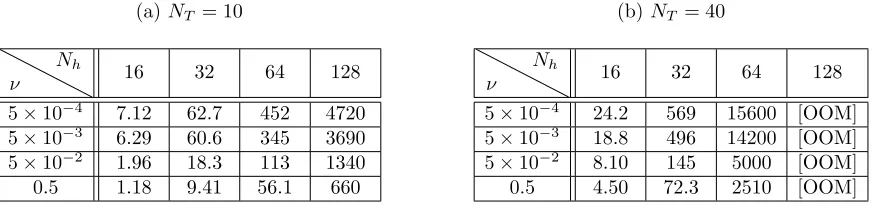
The purpose of this section is to discuss preconditioning strategies for the solution of this linear system. For the stationary setting discussed in [14], the solution of such a system via direct methods such as thebacklash (mldivide) command in MATLAB 1was feasible for relatively fine meshes (up to the order of 100 nodes per space dimension). However, as shown in Table 1, introducing a temporal dimension and thus increasing the degrees of freedom to N2
h ×NT significantly increases the computation time. Indeed, the use of backlashon
fine space and time grids – e.g. 1282space grid points and 40 time steps – requires an amount of RAM that is prohibitive on the machine used for our performance tests2, leading to “out of memory” errors. We mitigate this problem by exploring the solution of (5.1) via preconditioned iterative methods, which perform efficiently for finer space and time subdivisions and different viscosities.
(a)NT = 10
ν Nh
16 32 64 128
5×10⁻⁴ 7.12 62.7 452 4720 5×10⁻³ 6.29 60.6 345 3690 5×10⁻² 1.96 18.3 113 1340 0.5 1.18 9.41 56.1 660
(b)NT = 40
ν Nh
16 32 64 128
5×10⁻⁴ 24.2 569 15600 [OOM] 5×10⁻³ 18.8 496 14200 [OOM] 5×10⁻² 8.10 145 5000 [OOM] 0.5 4.50 72.3 2510 [OOM]
Table 1. MATLAB’sbackslashcomputation times (seconds) for a single linear system solved
in (4.9) within the Chambolle-Pock algorithm under a tolerance equal to 10−4in in normalized
`2-norm. For fine meshes [OOM] indicates an out of memory error for the tested architecture.
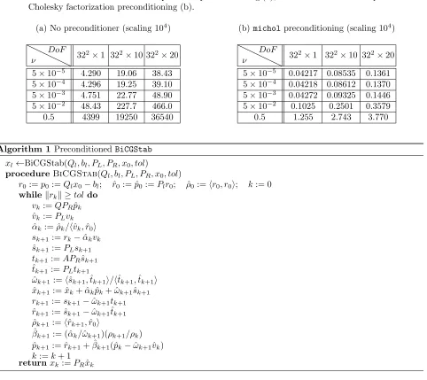
We begin by illustrating the difficulties associated to the conditioning of the system in (5.1). Table 2 shows the condition number of the system for different space-time discretizations and viscositiy values. Without any precoditioner, the condition numbers of different discretizations scale up to 108. The same Table shows that by selecting a suitable preconditioner, such as themodified incomplete Cholesky factorization [11] (michol in MATLAB), the conditioning of the system is improved by 4 orders of magnitude.
We have tested different choices of preconditioners and iterative methods for our problem. Since the matrix
Q in our setting is sparse, symmetric, and positive-definite, we have implemented an incomplete Cholesky factorizationwith diagonal scaling, amodified incomplete Cholesky factorization, and multigrid preconditioning. As for the choice of the iterative method, our tests included bothpreconditioned conjugate gradient(pcg), and thebiconjugate gradient stabilized method(BiCGStab). The interested reader will find in [36, Chapters 6 and 8] a thorough description of the aforementioned methods, and in the Appendix of this article performance tables for the different methods.
Our findings suggest that the use of an iterativepcgmethod, preconditioned by modified incomplete Cholesky factorization is satisfactory for small viscosities (ν ≤0.05). However, this algorithm fails to converge for high viscosity systems on refined grids (ν = 0.5, NT = 40, Nh ∈ {64,128}). Exchanging the pcgmethod by a BiCGStabalgorithm preconditioned by modified incomplete Cholesky factorization slows down the process on finer grids, but allows for convergence in the failure cases of pcg: ν= 0.5, NT = 40, Nh∈ {64,128}.
In order to deal with (and exploit) the anisotropy of the system introduced by high viscosities, we have devised an algorithm consisting in a multigrid preconditioner withBiCGStabiterations akin to that described in
1http://uk.mathworks.com/help/matlab/ref/mldivide.html
Algorithm 1. It is the only among the tested methods which performs consistently for different viscosities and space-time discretizations. We discuss its implementation and assess its performance in the following section 5.1.
Table 2. Condition numbers forQwithout preconditioning (a), and with modified incomplete
Cholesky factorization preconditioning (b).
(a) No preconditioner (scaling 104)
ν
DoF
322×1 322×10 322×20
5×10⁻⁵ 4.290 19.06 38.43 5×10⁻⁴ 4.296 19.25 39.10 5×10⁻³ 4.751 22.77 48.90 5×10⁻² 48.43 227.7 466.0 0.5 4399 19250 36540
(b)micholpreconditioning (scaling 104)
ν
DoF
322×1 322×10 322×20
5×10⁻⁵ 0.04217 0.08535 0.1361 5×10⁻⁴ 0.04218 0.08612 0.1370 5×10⁻³ 0.04272 0.09325 0.1446 5×10⁻² 0.1025 0.2501 0.3579 0.5 1.255 2.743 3.770
Algorithm 1 PreconditionedBiCGStab xl←BiCGStab(Ql, bl, PL, PR, x0, tol)
procedureBiCGStab(Ql, bl, PL, PR, x0, tol)
r0:=p0:=Qlx0−bl; rˆ0:= ˆp0:=Plr0; ρˆ0:=hr0, r0i; k:= 0
whilekrkk ≥toldo vk :=QPRpˆk
ˆ
vk :=PLvk
ˆ
αk:= ˆρk/hvˆk,ˆr0i
sk+1:=rk−αˆkvk
ˆ
sk+1:=PLsk+1
tk+1:=APRˆsk+1 ˆ
tk+1:=PLtk+1 ˆ
ωk+1:=hˆsk+1,ˆtk+1i/hˆtk+1,ˆtk+1i ˆ
xk+1:= ˆxk+ ˆαkpˆk+ ˆωk+1sˆk+1
rk+1:=sk+1−ωˆk+1tk+1 ˆ
rk+1:= ˆsk+1−ωˆk+1ˆtk+1 ˆ
ρk+1:=hrˆk+1,rˆ0i ˆ
βk+1:= ( ˆαk/ωˆk+1)(ρk+1/ρk)
ˆ
pk+1:= ˆrk+1+ ˆβk+1(ˆpk−ωˆk+1vˆk) k:=k+ 1
returnxk:=PRxˆk
5.1.
Multigrid preconditioner
We implement a multigrid preconditioned algorithm for solving (5.1). We refer the reader to [35] for an introduction and an overview of multigrid methods. We briefly review the main concepts behind the method. Consider two linear systemsA1¯x1=b1andA0x¯0=b0, stemming from two discretizations of a linear PDE over the grids G1 and G0, respectively. Assume also that G1 is a refinement of G0. Loosely speaking, the main idea of the method is that in order to find a good approximation of the solution ¯x1 on the finer grid, we first consider what is known as asmoothing step. This step consists in computing a few iteratesx1
1, . . . , x
η1 1 with a standard indirect method, such as Jacobi or Gauss-Seidel, and to define theresidualr1:=b1−A1x
η1
G0 the second system A0x¯0 =b0 with b0 = ˆr1, where ˆr1 is the restriction ofr1 to G0. Assuming that we can compute a good approximation of ¯x0, which we still denote by ¯x0, we then extend this solution toG1by using a linear interpolation. Callinge1 the resulting vector, we updatex
η1
1 by redefining it asx
η1
1 +e1 and we end the procedure by applying again a few iterations, sayη2, of a smoothing method initialized at xη1
1 . This last step is called post smoothing.
The previous paragraph introduced what is known as atwo grid iteration. If we consider more gridsG0,G1,. . .,
G`, where for each k= 0, . . . , `−1,Gk ⊆Gk+1, we can proceed similarly and obtain a better approximation
of the solution to A`x¯` = b`. As in the previous case, we begin with the finest grid G` and we perform η1 smoothing steps to obtain the residual r` := b`−A`x`η1 whose restriction to G`−1 is denoted by ˆr`. In this
grid we consider the system A`−1x`−1 = ˆr` and we perform again a smoothing step and a restriction of the
residual to G`−2. The procedure continues until we get to the coarsest grid G0, where the solution e0 to the corresponding linear system can be found easily (typically using a direct method). Next, the solution e1 on the grid G1 is corrected with the interpolation of e0. Another post smoothing is performed to the corrected solution on G1 and using its interpolation in the grid G2 we correct the previous solution on this grid. The smoothing, interpolation and correction iterations end once we arrive to the finest grid G` to obtain the final
approximation of ¯x`. The previous procedure is called a multigrid method with aV-cycle. An alternative, to
obtain a more accurate solution, is to proceed as before going fromG` to G`−1 and then fork =`−1, . . . ,1 to perform two consecutive coarse-grid corrections, instead of one as in the V-cycle. The resulting procedure is known as multigrid with a W-cycle. Finally, in between theV-cycle and the W-cycle, we have the F-cycle, where in the process of going from the coarsest grid to the finest one, if a grid has been reached for the first time, another correction with the coarser grids using aV-cycle is performed.
In our context, we use one cycle of the multigrid algorithm, which is a linear operator as a function of the residual on the finest grid, as a preconditioner for solving (5.1) with theBiCGStabmethod. SinceQis related to the finite difference discretization of the operator−∂2tt+ν2∆2−∆ andν is not necessarily small, as in [4], it is natural to consider the refinements of the grid only in the space variable (we refer the reader to [35] for semi-coarsening multigrid methods in the context of anisotropic operators). We suppose that the spatial mesh is such thatNh=H2`, withH >1 and`is a positive integer (in the numerical example in the next sectionH
will be equal to 2 or 3,H2 being the number of spatial points in the coarsest grid). Let us specify the main steps of the multigrid method we use as a preconditioner.
Hierachy of Grids: Semi-coarsened gridsGk with size (NT+ 1)H222k for allk= 0. . . `.
Cycle: We use the F-cycle.
Restriction operator: As in [4], in order to restrict the residual on the gridGk to the gridGk−1, we use
the second-order operatorRk:R(2
kH)2(NT+1)
→R(2k−1H)2(NT+1) defined by
(RkX)ni,j:=
1 16
4X2ni,2j+ 2(X2ni+1,2j+X2ni−1,2j+X2ni,2j+1+X2ni,2j−1)
X2ni−1,2j−1+X
n
2i−1,2j+1+X
n
2i+1,2j−1+X
n
2i+1,2j+1
! ,
forn= 0, . . . , NT,i,j = 1, . . . ,2k−1H.
Interpolation operator: We denote byIk:R(2
k−1H)2(N
T+1)→ R(2
kH)2(N
T+1) the interpolation operator
from the grid Gk−1 to the gridGk. We have chosen a standard bilinear interpolation operator in the
space variable, which is also a second-order operator and dual to the restriction operator (Ik = 4R∗k).
According to [12], the sum of the orders of Rk and Ik has to be at least equal to the degree of the
differential operator. In our context, both are equal to 4.
Linear systems on the different grids: The linear systems are defined by the matrices
where we recall thatAkandBkare the finite difference discretizations of∂t−ν∆ and div(·), respectively,
on the gridGk (see (3.1)).
Smoother: Here we have used Gauss-Seidel iterations in the lexicographic order. There is no reason for choosing the lexicographic order, other than its simplicity.
Solving the system on the coarsest gridG0: We can use an exact solver such asbacklashin MATLAB. Indeed, inG0the size of the system is really small with respect to the size of the system on the gridG`(in G0, we can even store the inverse ofQ0and inversion at this level just becomes a matrix multiplication).
The multigrid preconditoning procedure is summarized in Algorithm 2.
Algorithm 2 Multigrid Preconditioner forQ`x`=b` PL:y7→MultigridSolver(`,0, y,cycle)
xl←BiCGStab(Q`, b`, PL, Id, x0,tol)
procedureMultigridSolver(k, xk, bk,cycle) if k= 0then
xk ←Q−01bk else
xk ←Performη1 steps of Gauss-Seidel fromxk withbk as second member. xk−1←0
xk−1←MultigridSolver(k−1, xk−1, Rk(bk−Qkxk),cycle) if cycle is Wthen
xk−1←MultigridSolver(k−1, xk−1, Rk(bk−Qkxk),cycle) if cycle is Fthen
xk−1←MultigridSolver(k−1, xk−1, Rk(bk−Qkxk),V) xk ←xk+Ikxk−1
xk ←Performη2 steps of Gauss-Seidel fromxk withbk as second member. returnxk
5.2.
Numerical Tests
In this section we present a test case considered in [3], for which the stationary solution has been computed numerically in [14] using the primal-dual algorithm presented above.
The setting is as follows: we consider system (MFG) withg≡0 and
f(x, y, m) :=m2−H(x, y), H(x, y) = sin(2πy) + sin(2πx) + cos(2πx),
for all (x, y) ∈R2 andm ∈ R+. This means that in the underlying differential game modelled by (MFG), a
typical agent aims to get closer to the maxima of ¯H and, at the same time, he/she is adverse to crowded regions (because of the presence of them2term in f).
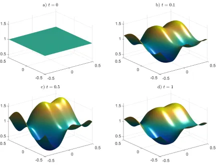
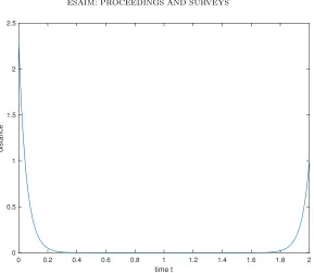
We first validate the dynamic behavior of our solution. Figure 1 shows the evolution of the mass at four different time steps. Starting from a constant initial density, the mass converges to a steady state, and then, whentgets close to the final timeT, the mass is influenced by the final cost and converges to a final state. This behavior is referred to asturnpike phenomenonin the literature [33]. It is illustrated by Figure 2, which displays as a function of timet the distance of the mass at timet to the stationary state computed as in [14]. In other words, denoting bym∞∈RNh×Nhthe solution to the discrete stationary problem and bym∈ Mthe solution to
the discrete evolutive problem, Figure 2 displays the graph ofk7→ km∞−mkk`2 =
h2P
i,j(m∞i,j−mki,j)2 1/2
,
Figure 1. Evolution of the density m obtained with the multi-grid preconditioner for ν = 0.5, T = 1, NT = 200 and Nh = 128. Att = 0.12 the solution is close to the solution of the
associated stationary MFG.
For the multi-grid preconditioner, Table 3 shows the computation times for different discretizations. It can be observed that finer meshes with 1283 degrees of freedom are solvable within CPU times which outperfom others methods shown in the Appendix and in [14]. Furthermore, the method is robust with respect to different viscosities.
From Table 3 we observe that most of the computational time is used for solving the second proximal operator (the third equality of (4.9)), which does not use a multigrid strategy but which is a pointwise operator (see Proposition 3.1 of [14]) and thus could be fully paralellizable.
Unlike the stationary case, low viscosities seem to make the algorithm be slightly slower. However, Table 4 shows that the average number of iterations of BiCGStabstays low regardless of the viscosity. Indeed Table 3 shows that more Chambolle-Pock iterations are needed to converge. The same behavior happens when we use a direct exact solver instead of the multi-grid preconditionedBiCGStabalgorithm.
0 0.2 0.4 0.6 0.8 1 1.2 1.4 1.6 1.8 2 time t
0 0.5 1 1.5 2 2.5
distance
Figure 2. Distance to the stationary solution at each timet∈[0, T], forν = 0.5, T = 2, NT =
200 andNh= 128. The distance is computed using the`2 norm as explained in the text. The
turnpike phenomenon is observed as for a long time frame the time-dependent mass approaches the solution of the stationary MFG.
(a) Grid with 64×64×64 points.
ν Total time Time first prox Iterations 0.6 116.3 [s] 11.50 [s] 20 0.36 120.4 [s] 11.40 [s] 21 0.2 119.0 [s] 11.26 [s] 22 0.12 129.1 [s] 14.11 [s] 22 0.046 225.0 [s] 23.28 [s] 39
(b) Grid with 128×128×128 points.
ν Total time Time first prox Iterations 0.6 921.1 [s] 107.2 [s] 20 0.36 952.3 [s] 118.0 [s] 21 0.2 1028.8 [s] 127.6 [s] 22 0.12 1036.4 [s] 135.5 [s] 23 0.046 1982.2 [s] 260.0 [s] 42
Table 3. Time (in seconds) for the convergence of the Chambolle-Pock algorithm, cumulative
time of the first proximal operator with the multigrid preconditioner, and number of iterations, for different viscoty values ν and two types of grids. Here we usedη1 =η2 = 2, T = 1 and a tolerance between two iterations of the Chambolle-Pock algorithm equal to 10−6in normalized
`2-norm.
the solution of a large-scale linear system at each iteration. We have overcome this difficulty by studying dif-ferent preconditioning strategies for the associated linear system. Overall, the multigrid preconditioner with a
BiCGStabiteration performs satisfactorily for different discretizations and viscosity values.
Acknowledgments. The third author wants to acknowledge funding within the ANR project MFG ANR-16-CE40-0015-01 operated by the French National Research Agency (ANR).
(a) iterations to decrease the residual by a factor 10−3.
ν 32×32×32 64×64×64 128×128×128 0.6 1.65 1.86 2.33 0.36 1.62 1.90 2.43 0.2 1.68 1.93 2.59 0.12 1.84 2.25 2.65 0.046 1.68 2.05 2.63
(b) iterations to solve the system with an error of 10−8.
ν 32×32×32 64×64×64 128×128×128 0.6 3.33 3.40 3.38 0.36 3.10 3.21 3.83 0.2 3.07 3.31 4.20 0.12 3.25 3.73 4.64 0.046 2.88 3.59 4.67
Table 4. Average number of iterations of the preconditionedBiCGStabwithη1=η2= 2, T =
1 and a tolerance between two iterations of the Chambolle-Pock algorithm equal to 10−6 in normalized`2-norm.
During the first phase of the project, the fifth author was affiliated to the Unit´e de Math´ematiques Pures et Appliqu´ees (UMPA) UMR CNRS 5669, of the ´Ecole Normale Sup´erieure de Lyon and to the Project-Team Beagle of the Inria Rhˆone-Alpes. He wishes to acknowledge funding within the framework of the LABEX MILYON (ANR-10-LABX-0070) of the Universit´e de Lyon, within the program ”Investissements d’Avenir” (ANR-11-IDEX-0007). In addition, his participation to this project has been partially supported by the European Research Council (ERC) under the European Union’s Horizon 2020 research and innovation program (grant agreement No. 639638). His participation to this project has also been partially supported by a CEMRACS 2017 scholarship.
The sixth author thanks the support from the PGMO project VarPDEMFG and from the ANR project MFG ANR-16-CE40-0015-01.
References
[1] Y. Achdou, F. Camilli, and I. Capuzzo-Dolcetta. Mean field games: numerical methods for the planning problem.SIAM J. Control Optim., 50(1):77–109, 2012.
[2] Y. Achdou, F. Camilli, and I. Capuzzo-Dolcetta. Mean field games: convergence of a finite difference method.SIAM J. Numer. Anal., 51(5):2585–2612, 2013.
[3] Y. Achdou and I. Capuzzo-Dolcetta. Mean field games: numerical methods.SIAM J. Numer. Anal., 48(3):1136–1162, 2010. [4] Y. Achdou and V. Perez. Iterative strategies for solving linearized discrete mean field games systems.Netw. Heterog. Media,
7(2):197–217, 2012.
[5] Y. Achdou and A. Porretta. Convergence of a finite difference scheme to weak solutions of the system of partial differential equations arising in mean field games.SIAM J. Numer. Anal., 54(1):161–186, 2016.
[6] G. Albi, Young-Pil Choi, M. Fornasier, and D. Kalise. Mean-field control hierarchy.Appl. Math. Optim., 76(1):93–175, 2017. [7] R. Andreev. Preconditioning the augmented Lagrangian method for instationary mean field games with diffusion.SIAM J.
Sci. Comput., 39(6):A2763–A2783, 2017.
[8] H. H. Bauschke and P.-L. Combettes.Convex analysis and monotone operator theory in Hilbert spaces. CMS Books in Math-ematics/Ouvrages de Math´ematiques de la SMC. Springer, Cham, second edition, 2017.
[9] J.-D. Benamou and G. Carlier. Augmented Lagrangian methods for transport optimization, mean field games and degenerate elliptic equations.J. Optim. Theory Appl., 167(1):1–26, 2015.
[10] A. Bensoussan, J. Frehse, and P. Yam.Mean field games and mean field type control theory. SpringerBriefs in Mathematics. Springer, New York, 2013.
[11] M. Benzi. Preconditioning techniques for large linear systems: A survey.J. Comput. Phys., 182(2):418–477, nov 2002. [12] A. Brandt. Rigorous quantitative analysis of multigrid. I. Constant coefficients two-level cycle withL2-norm.SIAM J. Numer.
Anal., 31(6):1695–1730, 1994.
[13] L. M. Brice˜no-Arias and P.-L Combettes. A monotone+ skew splitting model for composite monotone inclusions in duality. SIAM J. Optim., 21(4):1230–1250, 2011.
[14] L. M. Brice˜no-Arias, D. Kalise, and F. J. Silva. Proximal methods for stationary mean field games with local couplings.SIAM J. Control Optim., 56(2):801–836, 2018.
[16] P. Cardaliaguet. Notes on Mean Field Games: from P.-L. Lions’ lectures at Coll`ege de France.Lecture Notes given at Tor Vergata, 2010.
[17] P. Cardaliaguet. Weak solutions for first order mean field games with local coupling. In Analysis and geometry in control theory and its applications, volume 11 ofSpringer INdAM Ser., pages 111–158. Springer, Cham, 2015.
[18] P. Cardaliaguet and P. J. Graber. Mean field games systems of first order.ESAIM Control Optim. Calc. Var., 21(3):690–722, 2015.
[19] P. Cardaliaguet, P. J. Graber, A. Porretta, and D. Tonon. Second order mean field games with degenerate diffusion and local coupling.NoDEA Nonlinear Differential Equations Appl., 22(5):1287–1317, 2015.
[20] A. Chambolle and T. Pock. A first-order primal-dual algorithm for convex problems with applications to imaging.J. Math. Imaging Vision, 40(1):120–145, 2011.
[21] G. Chen and M. Teboulle. A proximal-based decomposition method for convex minimization problems. Math. Program., 64:81–101, 1994.
[22] D Gabay and B Mercier. A dual algorithm for the solution of nonlinear variational problems via finite element approximation. Comput. Math. Appl., 2(1):17–40, 1976.
[23] R. Glowinski and A. Marrocco. Sur l’approximation, par ´el´ements finis d’ordre un, et la r´esolution, par p´enalisation-dualit´e, d’une classe de probl`emes de Dirichlet non lin´eaires.Rev. Fran¸caise Automat. Informat. Recherche Op´erationnelle S´er. Rouge Anal. Num´er., 9(R-2):41–76, 1975.
[24] D.-A. Gomes, E. A. Pimentel, and V. Voskanyan.Regularity theory for mean-field game systems. SpringerBriefs in Mathematics. Springer, Cham, 2016.
[25] D.-A. Gomes and J. Sa´ude. Mean field games models - a brief survey.Dyn. Games Appl., 4(2):110–154, 2014.
[26] A. Lachapelle, J. Salomon, and G. Turinici. Computation of mean field equilibria in economics.Math. Models Methods Appl. Sci., 20(4):567–588, 2010.
[27] J.-M. Lasry and P.-L. Lions. Jeux `a champ moyen II. Horizon fini et contrˆole optimal.C. R. Math. Acad. Sci. Paris, 343:679– 684, 2006.
[28] J.-M. Lasry and P.-L. Lions. Mean field games.Jpn. J. Math., 2:229–260, 2007.
[29] A. R. M´esz´aros and F. J. Silva. A variational approach to second order mean field games with density constraints: the stationary case.J. Math. Pures Appl. (9), 104(6):1135–1159, 2015.
[30] A. R. M´esz´aros and F. J. Silva. On the variational formulation of some stationary second order mean field games systems. SIAM J. Mathematical Analysis, 50(1):1255–1277, 2018.
[31] N. Papadakis, G. Peyr´e, and E. Oudet. Optimal transport with proximal splitting.SIAM J. Imaging Sci., 7(1):212–238, 2014. [32] A. Porretta. Weak solutions to Fokker-Planck equations and mean field games.Arch. Ration. Mech. Anal., 216(1):1–62, 2015. [33] A. Porretta and E. Zuazua. Remarks on long time versus steady state optimal control. InMathematical Paradigms of Climate
Science, pages 67–89. Springer, Cham, 2016.
[34] R. T. Rockafellar. Duality and stability in extremum problems involving convex functions.Pacific J. Math., 21:167–187, 1967. [35] U. Trottenberg, C. W. Oosterlee, and A. Schuller.Multigrid. Academic Press, 2000.
[36] H. Wendland.Numerical Linear Algebra. Cambridge Texts in Applied Mathematics. Cambridge University Press, Cambridge, United Kindgom, first edition, 2017.
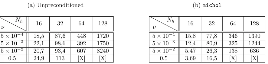
Appendix
(a) Unpreconditioned
ν Nh
16 32 64 128
5×10⁻⁴ 18,5 87,6 448 1720 5×10⁻³ 22,1 98,6 392 1750 5×10⁻² 20,7 93,4 607 8240 0.5 24,9 113 [X] [X]
(b)michol
ν Nh
16 32 64 128
5×10⁻⁴ 15,8 77,8 346 1390 5×10⁻³ 12,4 80,9 325 1244 5×10⁻² 5,47 26,3 138 636
0.5 3,69 16,5 [X] [X]
Table 5. Conjugate Gradient computation times (s). (a) Unpreconditioned. (b)
Precondi-tioned with modified incomplete Cholesky factorization. Time discretization: NT = 40. [X]
(a) Unpreconditioned
ν
Nh 8 16 32 64 128
5×10⁻⁴ 2.42 14.2 69.0 294 1210 5×10⁻³ 3.09 16.3 63.9 270 1210 5×10⁻² 1.41 12.9 61.3 389 5470 0.5 3.41 16.5 98.9 [X] [X]
(b)michol
ν
Nh 16 32 64 128
5×10⁻⁴ 15.7 80.4 412 1890 5×10⁻³ 12.2 82.2 369 1650 5×10⁻² 5.25 27.2 174 894
0.5 3.53 18.8 122 2120
Table 6. BiCGStab computation times (s). (a) Unpreconditioned. (b) Preconditioned with
modified incomplete Cholesky factorization. Time discretization: NT = 40. [X] indicates no