Please cite this article as: S. Mostafavian, S. R. Nabavianb, M. R. Davoodib, B. Navayi Neya, Output-only Modal Analysis of a Beam Via Frequency Domain Decomposition Method Using Noisy Data, International Journal of Engineering (IJE), IJE TRANSACTIONS C: Aspects Vol. 32, No. 12, (December 2019) 1753-1761
International Journal of Engineering
J o u r n a l H o m e p a g e : w w w . i j e . i rOutput-only Modal Analysis of a Beam Via Frequency Domain Decomposition
Method Using Noisy Data
S. Mostafavian*a, S. R. Nabavianb, M. R. Davoodib, B. Navayi Neyab
a Department of Civil Engineering, Payame Noor University (PNU), Tehran, Iran b Faculty of Civil Engineering, Babol Noshirvani University of Technology, Babol, Iran
P A P E R I N F O
Paper history:
Received 04 March 2019
Received in revised form 23 September 2019 Accepted 07 November 2019
Keywords:
Frequency Domain Decomposition Modal Parameters
Noise Level
Output-only Modal Analysis Simply Supported Beam
A B S T R A C T
The output data from a structure is the building block for output-only modal analysis. The structure response in the output data, however, is usually contaminated with noise. Naturally, the success of output-only methods in determining the modal parameters of a structure depends on noise level. In this paper, the possibility and accuracy of identifying the modal parameters of a simply supported beam in the presence of noise has been discussed. The output-only modal analysis method with frequency domain decomposition was used and output data with various noise levels were considered. Initially, finite element modal analysis was used to determine the modal parameters for the beam which were afterwards enforced as the reference modal parameters. Then, appropriate input was applied to the beam and the acceleration signals of different nodes were produced through finite element transient analysis. In order to simulate noisy data, noises with different power levels were generated and added to the signals. Finally, the modal parameters were obtained by frequency domain decomposition method. The results showed that the modal parameters corresponding to the first vibration mode could only be identified with acceptable validity at low to moderate noise levels, whereas for higher modes, the modal parameters can be correctly obtained even at high noise levels.
doi: 10.5829/ije.2019.32.12c.08
1. INTRODUCTION1
Modal parameters of structures, such as natural frequencies, damping ratios and mode shapes, have been used vastly in the past for numerous civil engineering applications. In order to obtain these parameters experimentally, there are two groups of modal analysis methods: input-output methods and output-only methods. Output-only modal analysis methods are mostly used due to their numerous advantages in comparison with other methods [1, 2]. One of the most common methods of output-only modal analysis is Frequency Domain Decomposition (FDD) which was proposed by Brincker [3]. In FDD method, matrices of Power Spectral Density (PSD) are formed with output data, after that the mode shapes and natural frequencies are extracted via Singular Value Decomposition (SVD) [4-6].
*Corresponding Author Email: [email protected] (S. Mostafavian)
employed a dynamic noise remover on the basis of the online wavelet concept for ignoring unwanted noise effects.
In spite of all these efforts, because of uncertainties in quality and quantity of noise in reality, it is not possible to entirely eliminate noise [9, 16]. Therefore, output-only methods rely on contaminated data with unknown noise level to identify modal parameters of structures. Although the effect of low levels of noise (up to 60%) were investigated in previous work [17, 18]. There was no study -to the best of our knowledge- in finding the maximum tolerable noise level; or equivalently minimum required value of signal to noise ratio (SNR) to identify the modal parameters via output-only methods. In this research, we will undertake this task. Moreover, we will evaluate the performance of the output-only method of FDD for various SNRs. For this purpose, a simply supported beam was chosen. An appropriate load was applied on the beam and acceleration signals of the beam were obtained using dynamic transient analysis. To generate noisy data, noises with different powers than signal power were added to the signals. Using these noisy data, the modal parameters of beams were obtained at various noise levels using FDD method. These parameters were compared with reference modal parameters of the beam that had been obtained by finite element modal analysis.
2. FREQUENCY DOMAIN DECOMPOSITION
METHOD
Among the nonparametric methods in the frequency domain, FDD has been used widely in output-only modal analysis because of its simplicity, dependability, and efficiency [3, 19]. However, FDD always requires the prior-selected natural frequencies as well as its strict hypotheses of uncorrelated white noise excitations and low structural damping. Output PSD matrix can be decomposed via fast-decayed decomposition methods such as SVD. This way, the spectral density reveals contributions of various modes of the structure. By analyzing the singular values, the auto PSD functions conforming to individual modes of a structure can be identified. In this method, the approximated mode shapes are obtained as the singular vectors at maximum location of any auto PSD function conforming to a mode. In what follows, the theoretical basis of the FDD method is summarized [20].
The pole-residue formula of the PSD matrix of output can be written as:
[𝐺𝑦𝑦(𝜔)] = ∑ (
[𝐴𝑘]
𝑗𝜔−𝜆𝑘+
[𝐴𝑘]∗
𝑗𝜔−𝜆𝑘∗+
[𝐵𝑘]
−𝑗𝜔−𝜆𝑘+
[𝐵𝑘]∗ −𝑗𝜔−𝜆𝑘∗) 𝑟
𝑘=1 (1)
where [𝐺𝑦𝑦(𝜔)] is the output PSD square matrix of dimension n in where n is the number of output data; r,
𝑗 and 𝜔 are number of desired modes, imaginary unit and natural frequency, respectively. [Ak] and 𝜆𝑘 are the kth residue output PSD matrix which is an n × n Hermitian matrix and pole of the kth mode, respectively (Superscript * defines complex conjugate). [𝐴
𝑘] and 𝜆𝑘 are given by:
[𝐴𝑘] = [𝑅𝑘][𝐶] ∑ (
[𝑅𝑠]𝐻 −𝜆𝑘−𝜆𝑠∗+
[𝑅𝑠]𝑇 −𝜆𝑘−𝜆𝑠) 𝑟
𝑠=1 (2)
𝜆𝑘= −𝜎𝑘+ 𝑗𝜔𝑑𝑘 (3)
where [Rk] is the residue of kth mode and equals to product
of modal participation vector {𝛾𝑘} and that of mode shape
{𝜙𝑘}. [𝐶] is PSD matrix of input which is constant;
𝜔𝑑𝑘and 𝜎𝑘 are natural frequency corresponding to the kth mode of damped system and the modal damping ratio, respectively (Superscripts H and T denote complex conjugate and transpose, respectively). Considering only the kth mode, Equation (2) turns into:
[𝐴𝑘] =[𝑅𝑘][𝐶][𝑅𝑘]𝐻
2𝜎𝑘 (4)
If the modal damping ratio is low, Equation (4) is dominant and the residue proportional to the mode shape vector can be achieved by the following equation:
[𝐴𝑘] ∝ [𝑅𝑘][𝐶][𝑅𝑘]𝐻= {𝜙𝑘}{𝛾𝑘}𝑇[𝐶]{𝛾𝑘}{𝜙𝑘}𝑇=
𝑧𝑘{𝜙𝑘}{𝜙𝑘}𝑇 (5)
where zkis the kth mode scaling factor. For a system with
low damping in which at a certain frequency, finite number of modes participate in the structure response, the output PSD matrix can be stated as:
[𝐺𝑦𝑦(𝜔)] = ∑ (𝑧𝑘
{𝜙𝑘}{𝜙𝑘}𝑇
𝑗𝜔−𝜆𝑘 +
𝑧𝑘∗{𝜙𝑘}∗{𝜙𝑘}∗𝑇
𝑗𝜔−𝜆𝑘∗ )
𝑘∈𝑆𝑢𝑏(𝜔) (6)
where 𝑘 ∈ 𝑆𝑢𝑏(𝜔) is the collection of participating modes at desired natural frequency. The singular value decomposition of the PSD matrix of output at natural frequency 𝜔 = 𝜔𝑖leads the following equation:
[𝐺̂𝑦𝑦(𝑗𝜔𝑖)] = [𝑉]𝑖[𝑁]𝑖[𝑉]𝑖𝐻 (7)
In Equation (7) the matrices [V]iand [N]i are unitary
matrix containing the singular vector {vij} and diagonal
matrix of singular values nij, respectively. Each mode
corresponds to a local maximum in the spectrum. When there is only one dominant mode, one term in Equation (6) remains, and the power spectral density matrix approximates to a matrix with rank equal to one:
𝐺̂𝑦𝑦(𝑗𝜔𝑖) = 𝑠𝑖{𝑣𝑖1}{𝑣𝑖1}𝐻𝜔𝑖→ 𝜔𝑘 (8)
Thus, the singular vector related to the first mode {vi1} gives a good estimate of mode shape as follows:
{𝜙̂} = {𝑣𝑖1} (9)
with the singular vectors related to the frequency lines near the maximum, the auto PSD function of the equivalent SDOF system is recognized near the maximum of the singular value diagram. Every line distinguished by a singular vector which offers a Modal Assurance Criterion (MAC) value greater than a suitable MAC rejection level, is related to the PSD function of SDOF system. The corresponding PSD function of SDOF system is utilized to obtain estimates of the damping ratios and natural frequencies [21].
3. MATHEMATICAL MODEL OF NOISE
Output-only modal analysis is performed using only the measured response of structure (𝑁𝑅(𝑡)). This response contains the structure response (𝑅(𝑡)) and the output noise (𝑁(𝑡)). The output noise consists of any undesired signals and physically may arise from measurement devices, sensors, etc. [22]. The simplest mathematical model for noise in data is the additive noise model [23]:
𝑁𝑅(𝑡) = 𝑅(𝑡) + 𝑁(𝑡) (10)
In this model, the output noise is demonstrated as a white Gaussian process with zero average [23] as shown in Equation (11) [25, 26]:
𝑁(𝑡) = 𝑅𝑀𝑆(𝑅(𝑡)) × 𝑁𝐿 × 𝑊(𝑡) (11)
where 𝑅𝑀𝑆(𝑅(𝑡)) is the root mean square of signals,
𝑊(𝑡) is a random function with the same dimension as
𝑅(𝑡), and 𝑁𝐿 is a constant that determines the noise level, The noise level is defined as the ratio of the root mean square (RMS) of the noise process to the RMS of the noise-free data. Noise level can also be represented by Signal to Noise Ratio (𝑆𝑁𝑅):
𝑆𝑁𝑅 =(𝑁𝐿)12 (12)
4. FINITE ELEMENT MODELING
As shown in Figure 1, a beam with simply supported condition was considered to study the noise level effect on output-only modal analysis. Finite element modeling was done in ANSYS1 software using BEAM 188 element which has six degrees of freedom at any nodes. A beam with a square cross section of 10 mm ×10 mm was modeled in 2-D space with 10 elements, each 100 mm long. The properties of material, namely elastic Young modulus, Poisson's ratio and mass density of the beam were considered 2×10¹¹ N/m2, 0.3 and 7850 (N.s2/m)/m3, respectively according to typical structural steel. Geometrical properties of the beam were selected so that the vibration modes of the beam were sufficiently separated.
1www.ansys.com
4. 1. Finite Element Modal Analysis The beam's
modal parameters were obtained by finite element modal analysis and were considered as its reference modal parameters. In this type of analysis, the following Eigen-value problem is solved [27]:
[𝐾 − 𝜔2𝑀]{𝜑} = 0 (13)
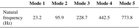
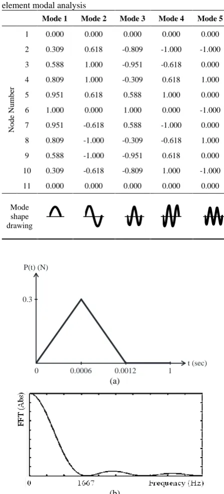
In Equation (13) matrices 𝐾 and 𝑀 are stiffness and mass, respectively; 𝜔 and 𝜑 are frequency and Eigen-vector of structure, respectively. The reference modal parameters (natural frequencies and mode shapes) of the beam for the modes from 1st to 5th were calculated and have been demonstrated in Tables 1 and 2.
4. 2. Applying Load and Transient Analysis To obtain the modal parameters corresponding to the first to fifth modes of this beam using FDD method, the frequency content of the applied load should include all frequencies of these modes. For this purpose, the load shown in Figure 2(a) is considered in which the load begins from zero at the time t = 0 and linearly reaches 0.3 N at 0.0006 s. It then returns to zero at 0.0012 s and then stays at zero until t = 1 s. Fast Fourier Transform (FFT) of the load can be observed in Figure 2(b) where due to symmetry, only one-half is displayed. In order to assure excitation of the first five modes of the beam, the first frequency with zero FFT value must be greater than the values of natural frequency of the fifth mode. Since this frequency is reversely proportional to time step in transient analysis, the time step should be sufficiently small. Time step of 0.0001 s was considered that corresponds to first zero FFT frequency of 1667 Hz, which is greater than the natural frequency related to the fifth mode of this beam, i.e. 773.8 Hz (Table 1).
In addition to appropriate frequency content for the applied load, the load position must not be located on the nodal points of the considered modes [28]. As can be observed in Table 2, appropriate locations to excite are nodes 2, 4, 8 and 10. The load was applied to this beam on node 4 in vertical direction. Through standard transient analysis in ANSYS, the vertical acceleration of nodes 2 to 10 were obtained.
11 10 9 8 7 6 5 4 3 2 1
Figure 1. Finite element model of beam with node numbers
TABLE 1. Natural frequencies of the beam extracted by modal
analysis of finite element model
Mode 5 Mode 4
Mode 3 Mode 2
Mode 1
773.8 442.5
228.7 95.9
23.2 Natural
TABLE 2. Mode shape values of the beam obtained by finite element modal analysis
Mode 5 Mode 4 Mode 3 Mode 2 Mode 1 0.000 0.000 0.000 0.000 0.000 1 N o d e N u mb er -1.000 -1.000 -0.809 0.618 0.309 2 0.000 -0.618 -0.951 1.000 0.588 3 1.000 0.618 -0.309 1.000 0.809 4 0.000 1.000 0.588 0.618 0.951 5 -1.000 0.000 1.000 0.000 1.000 6 0.000 -1.000 0.588 -0.618 0.951 7 1.000 -0.618 -0.309 -1.000 0.809 8 0.000 0.618 -0.951 -1.000 0.588 9 -1.000 1.000 -0.809 -0.618 0.309 10 0.000 0.000 0.000 0.000 0.000 11 Mode shape drawing 0.0012 0.0006 1 t (sec) 0.3 P(t) (N) 0 (a) (b)
Figure 2. (a) Excitation function and (b) its FFT (Not to
scale)
5. OUTPUT-ONLY MODAL ANALYSIS
As mentioned in Section 4, the acceleration signals
(𝑅(𝑡)) were obtained from the transient analysis of the beam. These signals are free of noise (zero noise level). Using these signals, the noise 𝑁(𝑡) was generated with different noise levels (𝑁𝐿) according to Equation (11).
1www.mathworks.com/products/matlab.html
By adding 𝑁(𝑡) to 𝑅(𝑡) according to Equation (10), the noisy data (𝑁𝑅(𝑡)) was generated which was used for output-only modal analysis by FDD method. The considered noise levels and the corresponding signal to noise ratios are shown in Table 3. Practically, the amount of noise in recorded response affects the accuracy of the estimated modal parameters [29, 30].
In the noise generation process, each ensemble is statistically independent from others. Moreover, in order to capture the effect of randomness and average out the results, the process should be repeated [24]. At each noise level, 100 noise ensembles 𝑁(𝑡) and consequently 100 noisy data 𝑁𝑅(𝑡) were generated. Output-only modal analysis by FDD method was performed using each of the 𝑁𝑅(𝑡)𝑠, and the average of the results obtained for each noise level is presented in the following. The process of noise generation, noisy data generation and Output-only modal analysis by FDD method were all performed in MATLAB1.
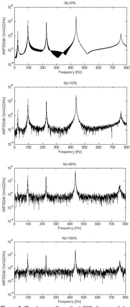
5. 1. Natural Frequencies Table 4 presents natural frequencies of the beam predicted using FDD method for different noise levels from NL=0 (noise free case) to NL=200%. The prediction error with respect to reference frequencies (Table 1) are shown in the last row of Table 4. As can be seen, FDD method predicted most natural frequencies of the beam accurately. Maximum error is -5.2% which belongs to mode 1. Moreover, natural frequency of mode 1 could not be identified at high noise levels; i.e. NL=100% and NL=200%. The error of most of the estimated natural frequencies is negative, which shows that they are underestimated.
As shown in Table 4, by increasing the noise level, the values of the natural frequencies identified using FDD method do not change. The results corroborate with those reported by Gkoktsi et al. [31]. In the frequency domain methods such as FDD, the natural frequency of a structure is estimated from the peak values of PSD
TABLE 3. Noise levels and corresponding signal to noise ratios
200% 100% 75% 50% 20% 10% 5% Noise Level (NL) 0.25 1 1.78 4 25 100 400 Nominal Signal to Noise Ratio (SNR)
TABLE 4. Natural frequencies (Hz) of the beam estimated via
FDD method Mode 5 Mode 4 Mode 3 Mode 2 Mode 1 Noise Level (%)
diagram. Despite the fact that different noise levels lead to different PSD diagrams, the peaks location or the values of natural frequencies of the structure do not change. This phenomenon is shown in Figure 3. 5. 2. Mode Shapes The first five mode shapes of the beam were obtained by FDD at various noise levels. For instance, mode shape values of the beam obtained at noise level 5% are shown in Table 5. In order to check accuracy of the obtained mode shapes, they will be compared with reference mode shapes obtained by finite element modal analysis (Table 2).
For the purpose of comparison, the MAC criterion is utilized. The MAC as a statistical index, shows a high sensitivity to large variations between two mode shape vectors, but it has relatively no sensitivity to small variations. This statistic indicator produces a good measure and degree of compatibility between two mode shapes. The MAC formulation is [32]:
𝑀𝐴𝐶(𝑟, 𝑞) = |{𝜑𝐴}𝑟𝑇{𝜑𝑋}𝑞|2
({𝜑𝐴}𝑟𝑇{𝜑𝐴}𝑟)({𝜑𝑋}𝑞𝑇{𝜑𝑋}𝑞)
(14)
where {𝜑𝐴}𝑟 is mode shape number 𝑟 from source 𝐴,
{𝜑𝑋}𝑞 is mode shape number 𝑞 from source 𝑋, and the superscript 𝑇 denotes transpose. The MAC values vary between zero and one; the one represents full compliance of two mode shapes [33].
Using Equation (14), the values of MAC between the five mode shapes of the beam obtained by FDD method and five reference mode shapes were calculated at various noise levels. For instance, these MAC values at noise level of 5% are presented in Figure 4. (At noise level of 5%, mode shape values in Table 5 and Table 2 were used for calculation of MAC values.) This figure shows that the values of MAC between the same mode shape numbers are equal to one and between different
TABLE 5. Mode shape values of the beam obtained by FDD
method at noise level of 5%
Mode 5 Mode 4
Mode 3 Mode 2
Mode 1
0.000 0.000
0.000 0.000
0.000 1
N
o
d
e
N
u
mb
er
0.999 1.000
0.813 0.620
0.312 2
-0.001 0.618
0.950 0.998
0.585 3
-0.996 -0.618
0.311 1.000
0.819 4
-0.001 -0.999
-0.588 0.618
0.956 5
1.000 -0.001
-1.000 0.003
1.000 6
-0.001 0.999
-0.586 -0.619
0.960 7
-0.999 0.618
0.307 -0.998
0.823 8
0.000 -0.618
0.951 -1.000
0.593 9
0.998 -0.999
0.809 -0.618
0.311 10
0.000 0.000
0.000 0.000
0.000 11
mode shape numbers are equal to zero. This means that the FDD uniquely identified all of the five mode shapes and there is no correlation between the mode shapes with different mode number. This result was also obtained for other noise levels.
Table 6 shows the values of MAC between the mode shapes obtained by FDD and the corresponding reference mode shapes at various noise levels (same mode
Figure 3. The Average Normalized PSD diagram of the
Figure 4. MAC values between all FDD mode shapes (at noise level of 5%) and all FEM mode shapes
number). The MAC values equal or close to one indicate that the FDD method appropriately extracted five mode shape vectors of the beam in the presence of noise. As shown in the table, as the noise level increases, the MAC values either decrease or remain constant. The lower values of the MAC for the first mode shape of the beam show that this mode of the beam was not extracted flawlessly in high noise levels. However, for the second to fifth mode shapes, the MAC value remains equal to one even at high noise levels which shows that these mode shapes were extracted with high accuracy.
The identified mode shapes of this beam via FDD method for the various noise levels have been drawn in Figures 5 to 8. As can be observed in Figures 5 and 6, that correspond to noise levels of 5% and 20% respectively, all of the five mode shapes were identified almost accurately. According to Table 5, the MAC values for these mode shapes at the same noise levels are equal to one. At noise levels of 75% and 200% in Figures 7 and 8, respectively, the second to fifth mode shapes are nearly perfect, but the first mode shape is clearly distorted. In Table 5, the values of MAC of second to fifth mode shape for all of the considered noise levels are equal to one. However, for the first mode shape, the MAC value decreases from 1.00 at noise level of 0, 5, 10 and 20% to 0.95 at noise level of 200%. Therefore, for the case being studied, MAC equal to or less than 0.99 means that the obtained mode shape is not reliable.
TABLE 6. values of MAC between FDD mode shapes and
corresponding FEM mode shapes
Modes 2 to 5 Mode 1
Noise Level (%)
1.00 1.00
0, 5,10,20
1.00 0.99
50, 75
1.00 0.97
100
1.00 0.95
200
As can be seen in Tables 4 and 6, the natural frequency of the first mode was obtained up to noise level of 75%, but its mode shape was only identified with good accuracy up to noise level of 20%. Therefore, identification of natural frequency of a mode does not necessarily guarantee that its mode shape will be identified correctly by FDD method.
Figure 5. The beam's mode shapes obtained via FDD at
noise level of 5%
Figure 6. The beam's mode shapes obtained via FDD at
noise level of 20%
Figure 7. The beam's mode shapes obtained via FDD at
Figure 8. The beam's mode shapes obtained via FDD at noise level of 200%
6. CONCLUSION
In the present work, a method of output-only modal analysis, namely FDD method, was utilized to identify modal parameters of a beam under noisy conditions. A finite element model was prepared for a simply supported beam. Applying a suitable dynamic load to the beam, the acceleration signals of the various points on the beam were obtained by transient analysis. Noise signals with different powers were added to the acceleration signals. Using these noisy acceleration signals, modal parameters of the beam were identified by FDD method. These identified modal parameters were then compared to reference ones that were obtained by finite element modal analysis method.
In noise free case, the FDD method could identify this beam's mode shapes and natural frequencies. The beam's natural frequency corresponding to the first mode was identified with more error in comparison to other modes. MAC values are equal to one in this case, which shows very good agreement between the identified mode shapes and the corresponding reference.
In the case of noisy signals, the beam's natural frequencies of all modes were obtained at all noise levels, except for the first natural frequency which was not identified for noise levels 100 and 200%. The first natural frequency could not be identified at very high noise levels. The natural frequencies of the beam, which were identified, show no change in comparison to the noise free case. The FDD was a powerful method for estimation of the beam's natural frequencies, because it identified the natural frequencies at the reasonably high noise levels. The inspection of the mode shapes obtained using FDD method under noisy conditions showed that all of the mode shapes were in very good agreement with reference mode shapes up to noise level of 20%. Up to this noise level, the calculated MAC values for all of the mode shapes are equal to one. For noise levels greater than 20%, accuracy of the first mode shape decreases
(MAC=0.99~0.95), but other mode shapes remain accurate (MAC=1.00). Therefore, the FDD method is more robust for prediction of natural frequencies in comparison to mode shapes. The amount of noise influenced properties of the first mode which is usually the most important vibration mode of a structure in practice. Because noise level is unknown in practice, the higher mode shapes identified by the FDD method are more reliable in comparison with the first mode shape.
7. REFERENCES
1. Giraldo, D. F., Song, W., Dyke, S. J. and Caicedo , J. M., “Modal identification through ambient vibration: comparative study”, Journal of Engineering Mechanics, Vol. 135, No. 8, (2009), 759-770.
2. Brincker, R. and Kirkegaard, P. H., “Special issue on Operational Modal Analysis”, Mechanical Systems and Signal Processing, Vol. 24, No. 5, (2010), 1209-1212. 3. Brincker, R., Zhang, L. and Andersen, P., “Modal
identification of output-only systems using frequency domain decomposition”, Smart Materials and Structures, Vol. 10, No. 3, (2001), 441-445.
4. Batel, M., “Operational modal analysis-Another way of doing modal testing”, Sound and Vibration, (2002), 22-27. 5. Andersen, P., Brincker, R., Goursat, M. and Mevel, L.,
“Automated modal parameter estimation for operational modal analysis of large systems”, in 2nd International Operational Modal Analysis Conference, 299-308, (2007). 6. Davoodi, M. R., Navayi Neya, B., Mostafavian, S. A.,
Nabavian, S. R. and Jahangiri, GH. R., “Determining minimum number of required accelerometer for output -only structural identification of frames”, in 7th International Operational Modal Analysis Conference, 279-284, 2017. 7. Mellinger, P., Döhler, M. and Mevel, L., “Variance estimation of
modal parameters from output-only and input/output subspace-based system identification”, Journal of Sound and Vibration, Vol. 379, (2016), 1–27.
8. Stephan, C., “Sensor placement for modal identification”,
Mechanical Systems and Signal Processing, Vol. 27, (2012) 461–470.
9. Wang, L., Song, R., Wu, Y. and Hu, W. “Statistically Filtering Data for Operational Modal Analysis under Ambient Vibration in Structural Health Monitoring Systems”, in 3rd International Conference on Industrial Engineering and Applications (ICIEA) MATEC Web Conference 2016, Vol. 68, 14010, (2016). 10. Makki Alamdari, M., Li, J. and Samali, B., “FRF-based damage
localization method with noise suppression approach”, Journal of Sound and Vibration, Vol. 333, No. 14, (2014), 3305–3320. 11. Peeters, B., Cornelis, B., Janssens, K. and Van Der Auweraer,
H., “Removing Disturbing Harmonics in Operational Modal Analysis”, in 2nd International Operational Modal Analysis Conference, 185-192, (2007).
12. Ingle, R. and Awale, R., “A unique approach of noise elimination from electroencephalography signals between normal and meditation state”, International Journal of Engineering-Transactions B: Applications, Vol. 31, No. 5, (2018), 719-728. 13. Bonness, W. K. and Jenkins, D. M., “Removing Unwanted Noise
from Operational Modal Analysis Data”, Topics in Modal Analysis, Vol. 10, (2015), 115–122.
International Journal of Engineering-Transactions B: Applications, Vol. 30, No. 2, (2017), 199-206.
15. Khoshnood, A. M., Khaksari, H., Roshanian, J. and Hasani, S. M., “Active noise cancellation using online wavelet based control system: numerical and experimental study”, International Journal of Engineering-Transactions A: Basics, Vol. 30, No. 1, (2017), 120-126.
16. Reynders, E. and De Roeck, G., “Reference-based combined deterministic-stochastic subspace identification for experimental and operational modal analysis”, Mechanical Systems and Signal Processing, Vol. 22, No. 3, (2008), 617–637.
17. Shi, Y., Li, Z. and Chang, C.C., “Output-only subspace identification of structural properties and unknown ground excitation for shear-beam buildings”, Advances in Mechanical Engineering, Vol. 8, No. 11, (2016), 1–15.
18. Yi, J.H. and Yun, C.B., “Comparative study on modal identification methods using output-only information”,
Structural Engineering and Mechanics, Vol. 17, No. 3-4, (2004), 445–466.
19. Tamura, Y., “Damping in buildings and estimation techniques”, in 6th Asia-Pacific Conference on Wind Engineering (APCWE-VI), 193-214, (2005).
20. Brincker, R., Zhang, L. and Andersen, P., “Output-Only Modal Analysis by Frequency Domain Decomposition”, in 25th International Conference on Noise and Vibration Engineering, 717-723, (2000).
21. Gade, S., Møller, N. B., Herlufsen, H. and Konstantin-Hansen H., “Frequency Domain Techniques for Operational Modal Analysis”, in 1st International Operational Modal Analysis Conference, 1-10, (2005).
22. Zhang, J., Prader, J., Grimmelsman, K. A., Moon, F., Aktan, A. E. and Shama, A., “Experimental Vibration Analysis for Structural Identification of a Long-Span Suspension Bridge”,
Journal of Engineering Mechanics, Vol.139, No.6, (2013), 748– 759.
23. Proakis, J.G. and Salehi, M., “Digital communications”, McGraw-Hill, Fifth edition, (2008).
24. Moaveni, B., Barbosa, A. R., Conte, J. P. and Hemez, F. M., “Uncertainty analysis of system identification results obtained for a seven-story building slice tested on the UCSD-NEES shake table”, Structural Control and Heath Monitoring, Vol. 21, No.4, (2014), 466–483.
25. Perry, M. J. and Koh, C. G., “Output-only structural identification in time domain: Numerical and experimental studies”,
Earthquake Engineering and Structural Dynamics, Vol. 37, No.4, (2008), 517–533.
26. Makki Alamdari, M., Samali, B., Li, J., Kalhori, H. and Mustapha, S., “Spectral-Based Damage Identification in Structures under Ambient Vibration”, Journal of Computing in Civil Engineering, Vol. 30, No. 4, (2016), 4015062.
27. He, J. and Fu, Z. F., “Modal Analysis”, Dehli: Butterworth HeinteMann, (2001).
28. Mostafavian, S. A., Davoodi, M. R. and Vaseghi Amiri, J., “Ball joint behavior in a double layer grid by dynamic model updating”,
Journal of Constructional Steel Research, Vol. 76, (2012), 28– 38.
29. Adeli, H. and Jiang, X., “Dynamic Fuzzy Wavelet Neural Network Model for Structural System Identification”, Journal of Structural Engineering, Vol. 132, No. 1, (2006), 102–111. 30. Moaveni, B. and Asgarieh, E., “Deterministic-stochastic subspace
identification method for identification of nonlinear structures as time-varying linear systems”, Mechanical Systems and Signal Processing, Vol. 31, (2012), 40–55.
31. Gkoktsi, K., Giaralis, A. and TauSiesakul, B., “Sub-Nyquist signal-reconstruction-free operational modal analysis and damage detection in the presence of noise”, in Proceeding of Sensors and Smart Structures Technologies for Civil, Mechanical, and Aerospace Systems 2016, 980312, (2016).
32. Pastor, M., Binda, M. and Harčarik, T., “Modal Assurance Criterion”, Procedia Engineering, Vol. 48, (2012), 543-548. 33. Allemang, R.J., “The modal assurance criterion - Twenty years of
Output-only Modal Analysis of a Beam Via Frequency Domain Decomposition
Method Using Noisy Data
S. Mostafaviana, S. R. Nabavianb, M. R. Davoodib, B. Navayi Neyab
a Department of Civil Engineering, Payame Noor University (PNU), Tehran, Iran b Faculty of Civil Engineering, Babol Noshirvani University of Technology, Babol, Iran
P A P E R I N F O
Paper history:
Received 04 March 2019
Received in revised form 23 September 2019 Accepted 07 November 2019
Keywords:
Frequency Domain Decomposition Modal Parameters
Noise Level
Output-only Modal Analysis Simply Supported Beam
هدیکچ
یجورخ لادوم زیلانآ
-هداد زا هدافتسا اب اهنت یم ماجنا هزاس کی یجورخ یاه
.دوش هداد نیا ًلاومعم اه هزاس خساپ لماش هب
هارمه شور تیقفوم .دنتسه زیون یرادقم یجورخ یاه
زیون نازیم هب یگتسب هزاس لادوم یاهرتماراپ نییعت رد اهنت رد
هداد نیا رد .دراد یجورخ یاه ،هلاقم
کما نا نییعت هداس رس ود ریت کی لادوم یاهرتماراپ اهنآ تقد زین و
دوجو ریثأت تحت
زیون هتفرگ رارق یسررب دروم .تسا
زا یجورخ لادوم زیلانآ شور
هیزجت یاهنت سناکرف هزوح
هدافتسا دش هداد و یاه
فلتخم زیون نازیم اب یجورخ ظاحل
دیدرگ نآ قیرط زا ریت لادوم یاهرتماراپ ادتبا رد . دودحم یازجا لادوم زیلا
ییعت ن هدش و
اونع هب ن عجرم لادوم یاهرتماراپ تفرگ رارق هدافتسا دروم
. لانگیس و دش لامعا ریت هب یبسانم یدورو سپس باتش یاه
رد
هرگ هداد دیلوت یارب .دمآ تسدب دودحم یازجا ینامز هچخیرات لیلحت قیرط زا فلتخم یاه ناوت اب یاهزیون ،یزیون یاه
لانگیس هب و دیلوت فلتخم .دش هفاضا اه
هیزجت شور قیرط زا ریت لادوم یاهرتماراپ تیاهن رد سناکرف هزوح
.دیدرگ هبساحم
ناشن هلصاح جیاتن دنداد
دوم نیلوا لادوم یاهرتماراپ
یشاعترا ، ییاسانش لوبق لباق تقد اب طسوتم ات نییاپ زیون نازیم رد اهنت
یم رد ،دوش اهدوم یارب هکیلاح لباق حیحص روط هب لااب زیون نازیم رد یتح لادوم یاهرتماراپ ،رتلااب ی
لوصح .دنتسه