Solving a System of Linear Equations by Homotopy Analysis Method

University of Mazandaran, Iran http://cjms.journals.umz.ac.ir ISSN: 1735-0611

CJMS.2(1)(2013), 77-84

Solving a System of Linear Equations by Homotopy Analysis Method

M. Bayat 1 and Z. Khatami2

1 _{Department of Mathematics, Zanjan Branch, Islamic Azad}

University, Zanjan, Iran

2 _{Department of Mathematics, Zanjan University, Zanjan, Iran}

Abstract. In this paper, an efficient algorithm for solving a sys-tem of linear equations based on the homotopy analysis method is presented. The proposed method is compared with the classical Jacobi iterative method, and the convergence analysis is discussed. Finally, two numerical examples are presented to show the effec-tiveness of the proposed method.

Keywords: Homotopy analysis method, System of Linear Equa-tions, Jacobi iterative method.

1. INTRODUCTION

The homotopy analysis method (HAM) was proposed by Liao in His works [1-3]. In recent years, this method has been successfully em-ployed to solve many types of linear or linear, homogeneous or non-homogeneous, equations and systems of equations as well as problems in science and engineering [3-9]. The homotopy analysis method con-tains the auxiliary parameter~i which provides us, with a simple, way adjusting and controling the convergence region and rate of convergence of the resulted series solution.

1_{Corresponding author: baayyaatt@gmail.com}

In most cases, the homotopy analysis method leads to a very rapidly convergent series solution, and usually only a few iterations are suffi-cient to arrive at a very accurate solution, specially when the auxiliary parameter~i and the base functions are properly chosen.

In this paper, the homotopy analysis method is used to find the solution of the linear system Ax=b. The convergence of the proposed method is also studied.

2. REVIEW OF THE HOMOTOPY ANALYSIS METHOD

Consider the following system of equations

Ni[u1(r, t),· · ·, un(r, t)] = 0, (i= 1,2,· · · , n) (2.1)

subject to the initial conditions:

uk(r, t) =ck (k= 1,2,· · ·, n),

whereN_i are linear or nonlinear operators,r and tdenote the indepen-dent variables andui(r, t) are unknown functions. By means of general-izing the traditional homotopy analysis method, Liao [1-4] constructed the so called zero-order deformation equations for i= 1,2,· · ·, n (1−p)Li[ϕi(r, t;p)−ui0(r, t)] =p~iHi(r, t)Ni[ϕ1(r, t;p),· · ·, ϕn(r, t;p)],

(2.2) where p ∈ [0,1] is the embedding parameter, ~i 6= 0 are non-zero aux-iliary parameters for i = 1,2,· · ·, n, Hi(r, t) 6= 0 non-zero auxiliary functions,L_i’s are auxiliary linear operator with the following property fori= 1,2,· · · , n

Li[ϕi(r, t)] = 0, when ϕi(r, t) = 0. (2.3)

Also ui0(r, t) are initial guesses of ui(r, t) and ϕi(r, t;p) are unknown functions, respectively. It is important, that one has a great freedom to choose auxiliary things in the homotopy analysis method. Obviously, when p= 0 and p= 1 we have

ϕi(r, t; 0) =ui0(r, t), ϕi(r, t; 1) =ui(r, t), (i= 1,2,· · · , n). (2.4)

Thus, as p increases from 0 to 1, the solutions ϕi(r, t;p) vary from the initial guesses ui0(r, t) to the solutions ui(r, t). Expanding ϕi(r, t;p) in Taylor series with respect top, we have

ϕi(r, t;p) =ui0(r, t) + +∞

X

m=1

uim(r, t)pm, (i= 1,2,· · ·, n), (2.5)

where

uim(r, t) = 1 m!

∂mϕi(r, t;p) ∂pm

If the auxiliary linear operator, the initial guess, the auxiliary parameter ~i, and the auxiliary function are so properly chosen, the series (5) converges atp= 1, and so we have

uim(r, t) =ui0(r, t) + +∞

X

m=1

uim(r, t) (i= 1,2,· · · , n). (2.7)

Define the vectors

−→

uin={ui0(r, t), ui1(r, t),· · · , uin(r, t)} (i= 1,2,· · · , n). (2.8)

Differentiating (7)m times with respect to the embedding parameter p and then setting p = 0 and finally dividing them by m!, we obtain the mth-order deformation equation fori= 1,2,· · ·, n:

L_i[uim(r, t)−χmui,m−1(r, t)] =~iHi(r, t)Rim(−→u1,m−1,· · · ,−→un,m−1, r, t),

(2.9) where

Rim(−→u1,m−1,· · ·,−→un,m−1, r, t) =

1 (m−1)!

∂m−1_N

i[ϕ1(r, t;p),· · · , ϕn(r, t;p)] ∂pm−1

p=0

(2.10) and

χm =

0 m≤1,

1 m >1. (2.11)

3. SYSTEM OF LINEAR EQUATIONS

Consider the linear system Ax=b, where A is an n×n matrix, b

is a known vector and x is the unknown vector of variables. It is also assumed that the system has a unique solution. The i-th equation of this system can be expressed as follows:

ai,1x1+· · ·+ai,i−1xi−1+ai,ixi+ai,i+1xi+1+· · ·+ai,nxn=bi. (3.1)

Without loss of generality, suppose that ai,i 6= 0. It is now possible to obtain xi from (12), which concludes that

xi = bi ai,i

− 1

ai,i

ai,1x1+· · ·+ai,i−1xi−1+ai,i+1xi+1+· · ·ai,nxn

. (3.2)

In the following, we will use HAM to find the solution of (13). It is concluded from (1) and (13) that

Ni[x1,· · ·, xn] =xi− bi aii

+ 1 aii

ai1x1+· · ·+ai,i−1xi−1+ai,i+1xi+1+· · ·ainxn

In (8) and (9) for all i we define Hi(r, t) = 1, uim(r, t) = xim, ~i = ~, andL_i the identity linear operator. Also, we consider the functionϕi(p) as follows:

ϕi(p) =xi0+ +∞

X

m=1

ximpm (i= 1,2,· · ·, n),

xim= 1 m!

∂mϕi(p) ∂pm p=0 . (3.4)

Themth-order deformation equation is obtained as

xim−χmxi,m−1=~Rim(−→x1,m−1,· · ·,−→xn,m−1), (3.5)

where

Rim(−→x1,m−1,· · ·,−→xn,m−1) =

1 (m−1)!

∂m−1Ni[ϕ1(p),· · ·, ϕn(p)]

∂pm−1

p=0 = 1

(m−1)! ∂m−1

ϕi(p)−_aiibi +_aii1 Pn

j=1 j6=i

aijϕj(p)

∂pm−1

p=0 = 1

(m−1)! ∂m−1

xi0+P+_m∞₌₁ximpm−_aiibi +_aii1 Pnj=1 j6=i

aij

xj0+P+_m∞₌₁xjmpm

∂pm−1

p=0 =   

xi0− _aiibi + _aii1

Pn

j=1 j6=i

aijxj0 m= 1,

xi,m−1+_aii1

Pn

j=1 j6=i

aijxj,m−1 m >1.

fori= 1,2,· · · , n. Assumingxi0= _aiibi fori= 1,· · ·, n, we have







xi1= _aii~ Pnj=1 j6=i

aijxj0

xi,m = (1 +~)xi,m−1+_aii~ Pnj=1 j6=i

aijxj,m−1 (m≥2).

(3.6)

In order to make a better comparison between this method and the Jacobi iterative method [10] we rewrite the HAM scheme in matrix form. Toward this end, let D stands for the diagonal matrix whose diagonal elements are the same as A. It is also assumed that −L is the strictly lower-triangular part ofA, and−Uis the strictly upper-triangular part of A. Using this notations, A can be written as A=D−L−U and the equationAx=b, or equivalently (D−L−U)x=b, yields

Dx= (L+U)x+b, (3.7)

which can further be written as

This results the following matrix form for the homotopy analysis method:







x(0) _=D−1_b

x(1) =~D−1(L+U)x(0) (m= 2,3,· · ·)

x(m) =TA(~)x(m−1),

(3.9)

whereTA(~) = (1 +~)I+~D−1(L+U).

Note that the iteration matrix of the homotopy analysis method is simi-lar to the Jacobi iterative method. But, the initial value of the homotopy analysis method is D−1b, while the initial value of the Jacobi iterative method is usually assumed to be the zero vector.

4. CONVERGENCE ANALYSIS OF THE PROPOSED METHOD

According to (20), it can be easily shown that

x(m) =TA(~)

m−1

x(1), (m= 2,3,· · ·). (4.1)

Hence, the solution can be written as

x=x(0)+x(1)+x(2)+x(3)+· · · , (4.2) or equivalently,

x=x(0)+

h

I+TA(~) + (TA(~))2+ (TA(~))3+· · ·

i

x(1). (4.3)

Now, the following theorem can be proved.

Theorem 4.1. The sequence

x[m]=x(0)+ m

X

k=0

(TA(~))kx(1), (m= 0,1,2,· · ·), (4.4)

is a Chauchy sequence if

kT_A(~)k<1. (4.5)

Proof. We must show that

lim m→∞

x[m+p]−x[m] = 0.

In order to show this, first we write

x[m+p]−x[m]=

" _p X

k=1

(TA(~))m+k

#

x(1),

which yields

x[m+p]−x[m]

≤ kx(1)k

p

X

k=1

Letγ =T_A(~) , then

x[m+p]−x[m]

≤ kx(1)kγm

p

X

k=1

γk≤ kx(1)kγ

p+1₋₁

γ−1

γm.

Now ifγ <1, then we have

lim m→∞

x[m+p]−x[m]

≤ kx(1)k

γp+1−1

γ−1

lim m→∞γ

m_.

Hence, we obtain

lim m→∞

x[m+p]−x[m] = 0,

which completes the proof.

5. NUMERICAL RESULTS

In this section, two examples are presented. In the first example a system of linear equations is solved by the homotopy analysis method and the Jacobi iterative method and then the results are compared with each other.

Example 5.1. In this example, we approximate the solution of the system







10x1+x2+x3= 24 −x1+ 20x2+x3 = 21

x1−2x2+ 100x3 = 300

where the exact solution of which is x = (x1, x2, x3)t = (2,1,3)t. The

comparison will be made by applying the two methods separately.

(i)The Homotopy Analysis Method

From (20), we have x1,0 = 24₁₀,x2,0 = 21₂₀, andx3,0= 300₁₀₀,







x1,m+1 = (1 +~) + ₁₀~ x2,m+x3,m

x2,m+1 = (1 +~) + ₂₀~ −x1,m+x3,m

(m= 0,1,2,· · ·) x3,m+1 = (1 +~) + ₁₀₀~ x1,m−2x2,m

For ~=−1 and ~=−0.99, the solutions in the first five iterations are listed in Tables 1 and 2 respectively .

(ii)The Jacobi iterative method

We convert Ax = b into the form x = T x+c. To do this, solve i-th equation for xi, i= 1,2,3 to obtain:







x1= ₁₀1(−x2−x3) +24₁₀,

x2= ₂₀1(x1−x3) +21₂₀,

x3= ₁₀₀1 (−x1+ 2x3) + 300₁₀₀.

For an initial approximation, we let x(0) = (0,0,0). Approximate solu-tions are presented in Table 3.

Table 1. The homotopy analysis method for~=−1

Iteration x1 x2 x3

0 2.400000 1.050000 3.000000

1 1.995000 1.020000 2.997000

2 1.998300 0.999900 3.000450

3 1.999965 0.999893 3.000015

4 2.000009 0.999998 2.999998

5 2.000000 1.000001 3.000000

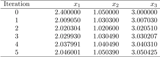
Table 2. The homotopy analysis method for~=−0.99

Iteration x1 x2 x3

0 2.400000 1.050000 3.000000

1 2.009050 1.030300 3.007030

2 2.020304 1.020600 3.020510

3 2.029930 1.030490 3.030207

4 2.037991 1.040490 3.040310

5 2.046001 1.050390 3.050425

Table 3. Jacobi method

Iteration x1 x2 x3

0 0.000000 0.0000000 0.000000

1 2.400000 1.0500000 3.000000

2 1.995000 1.0200000 2.997000

3 1.998300 0.9999000 3.000450

4 1.999965 0.9998925 3.000015

5 2.000009 0.9998975 2.999998

6 2.000000 1.0000010 3.000000

Considering the Tables 1 and 2, we see that the two Tables are the same for the first rows. In other words, if the initial values in the Jacobi iterative method are selected x(0) = (24₁₀,21₂₀,300₁₀₀), then the Adomian decomposition method and the Jacobi iterative method are exactly the same [4].

Example 5.2. The aim of this example is to approximate the solution of the system







4x1+x2−x3 = 7 −x1+ 6x2+ 2x3= 9

x2−3x3 = 5

where the exact solution of which isx= (x1, x2, x3)t= (1,2,−1)t. From

(20), we havex1,0 = 7₄,x2,0= 9₆, and x3,0 =−5₃. The six term

approxi-mation of the solution vectorx is

x'x0+x1+· · ·+x5,

which yields

~=−1.1⇒xt'[0.92092,2.06033,−0.93491], ~=−0.9⇒xt'[1.07051,1.95926,−1.06693], ~=−1.0⇒xt'[0.99565,2.00984,−1.00087].

References

[1] S.J. Liao, The proposed homotopy analysis technique for the solution of nonlinear problems, PhD thesis, Shanghai Jiao Tong University, 1992.

[2] S.J. Liao,An approximate solution technique which does not depend upon small parameters: a special example, Int J Nonlinear Mech, 30 (1995), 371-380.

[3] S.J. Liao,Homotopy analysis method: a new analytical technique for non-linear problems,Commun Nonlinear Sci Numer Simulat,2(1997), 95-100. [4] S.J. Liao, Beyond perturbation: introduction to the homotopy analysis

method,Boca Raton: CRC Press, Chapman & Hall; 2003.

[5] H. Jafari, S. Seifi, A. Alipoor and M. Zabihi,An iterative method for solving linear and nonlinear fractional diffusion-wave equation,J. Nonlinear Fract Phenom Sci. Eng., in press.

[6] H. Jafari and S. Seifi,Homotopy analysis method for solving linear and non-linear fractional diffusion-wave equation, Commun Nonlinear Sci. Numer Simulat, 14(2009), 2006-2012.

[7] A.S. Bataineh, M.S.M. Noorani and I. Hashim,Approximate analytical solu-tions of systems of PDEs by homotopy analysis method, J Comput Math Appl,55 (2008), 2913-2923.

[8] H. Xu, S.J. Liao and X.C. You,Analysis of nonlinear fractional partial differ-ential equations with the homotopy analysis method,Commun Nonlinear Sci Numer Simulat, 14(2009), 1152-1156.