Recent progress on Frequency Difference Electrical Impedance Tomography

(1)

H. Ammari, Editor

RECENT PROGRESS ON FREQUENCY DIFFERENCE ELECTRICAL

IMPEDANCE TOMOGRAPHY

Jin Keun Seo

1

_{, Bastian Harrach}

2

_{and Eung Je Woo}

3

Abstract. Although time-difference EIT(tdEIT) has shown promise as a medical EIT imaging tech-nique such as monitoring lung function, static EIT has suffered from forward computational model errors including boundary geometry and electrode positions uncertainty combined with the ill-posed and highly nonlinear nature of the corresponding inverse problem. Since 1980s, there has been great endeavor to create forward computational models with the necessary accuracy required for EIT recon-struction, but these efforts were not successful in clinical environment. This is the main reason why we consider frequency-difference EIT (fdEIT) where we take advantage of frequency dependance of biological tissue by injecting currents with at least two different frequencies. In this article, we review recent progress in fdEIT.

Introduction

Viewing the human body as a composition of resistance and reactance, we can characterize electrical prop-erties of a living organism by measuring the ratio of an externally applied current to the resulting voltage. The electrical conductivity and permittivity values of biological tissues and organs change with their physiological and pathological conditions and thus provide useful diagnostic information. Hence, the non-invasive measure-ment of the bioelectric impedance inside the human body has been an important research topic in biomedical engineering.

Electrical Impedance Tomography(EIT) is a non-invasive imaging technique which aims to provide the cross-sectional distribution of electrical impedance inside the human body. In EIT, we attach surface electrodes (typically 8 to 256) on the boundary of the subject, inject linearly independent patterns of sinusoidal currents in the frequency range of 50Hz to 500kHz, and measure the induced complex voltages. Since the relationship between the applied current and the resulting voltage data provide the electrical propensity of the subject, we use all available distributed current patterns and the measured voltage data set to reconstruct cross-sectional images of the conductivity and/or permittivity distribution inside the subject. This EIT technique has received considerable attention over the past two decades. Several review papers describe numerous aspects of the EIT technique [5, 8, 24, 29, 37], and mathematical theory was developed to support EIT system [1, 10, 16, 23, 26, 27, 34–36].

In order to make a static EIT image reconstruction algorithm reliable as a medical EIT imaging technique, one needs to construct a forward computational model with the same geometry as the imaging object and the accurate electrode positions. Barber and Brown [15] pointed out that, in order to obtain useful EIT images,

1 _{Department of Computational Science & Engineering, Yonsei University, Korea}

2 _{Institute for Mathematics, Johannes Gutenberg-Universit¨}_{at, 55099 Mainz, Germany}

3 _{College of Electronics and Information, Kyung Hee University, Korea}

c

EDP Sciences, SMAI 2009

(2)

electrode positions should be determined within 0.1mm accuracy when electrodes are spaced 100mm apart. In clinical environments, achieving this accuracy in the forward modeling would be very difficult with a reasonable cost. This requirement of accuracy is related to the fundamental shortcomings of the corresponding inverse problem that has low sensitivity of measured data to a local change of conductivity, relatively high sensitivity of measured data to boundary geometry errors and electrode positions uncertainty, and high nonlinearity between data and internal conductivity distribution. Without dealing with these undesirable influences of modeling errors, the static EIT imaging cannot be successful in clinical environments.

In time difference EIT(tdEIT), we reconstruct the temporal change of the complex conductivity distribution using the time difference between two consecutive measured voltage data sets. tdEIT takes advantage of alleviating modeling errors contained in the voltage data set since the time difference between two consecutive boundary voltage data sets may cancel out boundary geometry errors and electrode positions uncertainty. tdEIT imaging was first proposed by Barber and Brown [4] using the backprojection method, and Cheneyet al.[9] used the one-step Newton method for tdEIT. tdEIT has been applied to the monitoring of heart function, blood flow, and emptying of the stomach. Most of the published researches on phantom experiments essentially were based on tdEIT techniques since their results used the measured voltage data set corresponding to a homogeneous background instead of using a computed voltage data set for a forward model [15, 25, 28].

In the case of tumor imaging including breast tumor and in stroke type detection, we cannot use the tdEIT method since a reference measurement of the voltage data is not available, and any method using the computed reference voltage with a forward model can not be reliable due to the modeling errors mentioned before. To deal with this problem, we consider frequency-difference EIT (fdEIT) where we inject currents with at least two different frequencies. In fdEIT, it is essential to use the weighted difference of boundary voltage data to produce an image of frequency-dependent changes of the internal complex conductivity distribution. Compared with tdEIT, fdEIT does not require a reference data set from the past.

This lecture note focuses on robust reconstructions (instead of high resolution) under practical environments having various technical limitations due to the data collection equipment and the fundamental limitations of its inherent nature. We describe the mathematical formulation of single and multi-frequency EIT in clinical environments, image reconstruction algorithms, measurement techniques, and show examples of EIT images.

1. _{Inverse problems of fdEIT}

1.1. fdEIT model

The human body can be viewed as a mixture of resistors and capacitors. We begin with reviewing a circuit model containing resistors, capacitors, and a cosinusoidally time-varying current source. If the current source in the circuit is given by Iω(t) =Icos(ωt) whereI is the amplitude andω is the angular frequency, then the resulting voltageVω(t) between two points in the circuit is also time-harmonic with the same angular frequency

ω. The relation betweenIω(t) andVω(t) is given by

RIω˙ (t) + 1

CIω= ˙Vω(t),

where R is the total resistance of the circuit and C is the total capacitance. R and C depend on the circuit topology, the position of the current source and the two points between which the voltage is measured. The resulting voltage can be written as

Vω(t) =RIcos(ωt) + I

(3)

where ˜Vω = q

(RI)2₊ I2

C2_ω2 is the amplitude and the phase shift φω satisfies tanφω =

1

RCω and 0≤φω ≤ π

2.

Introducing the complex potential differenceuω= ˜Vωe−iφ, we have

R+ 1

iωC

Ieiωt=uωeiωt, or R+ 1

iωC = uω

I .

Hence, we can determine the complex total impedanceZ:=R+ 1

iωC from the relationship betweenI anduω.

Next, we consider a two or three dimensional model inverse problem in EIT. Let the subject occupy a two or three dimensional region Ω bounded by its surface∂Ω. Assume that the boundary∂Ω is connected and smooth. In EIT, we attach copper electrodes E1, . . . ,EL on ∂Ω. With these L surface electrodes, we usually applyL

different time-harmonic electrical currents using the Lpairs of electrodes (Ej,Ej+1), j = 1, . . . , Lto inject the

sinusoidal currentIcos(ωt). Here, we denoteEL+1=E1. Although the injection current using the pair (EL,E1)

is a linear combination of the other injection currents using pairs (Ej,Ej+1), j = 1, . . . , L−1 mathematically,

we always inject this redundant current for compensation of systematic errors in practice.

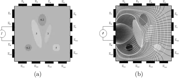
0.2 5 0.2 5 3 I E1 E2 E3 E16 E15 E14 E8 E9 E13 E12 E11 E10 E7

E6 E5 E4

(a) I E1 E2 E3 E16 E15 E14 E8 E9 E13 E12 E11 E10 E7

E6 E5 E4

(b)

Figure 1. (a) Surface electrodes E_j, j = 1, . . . ,16, are attached on the boundary of a simplified

rectangular model with a given conductivity distribution. (b) We inject the AC currentIcos(ωt) using the electrodesE₈ andE₉.

Let Vj

ω(r, t), be the corresponding electric potential to the current Icos(ωt) injected through the pair of

electrodes (Ej,Ej+1). WritingV_ωj(r, t) =<{uj_ω(r)eiωt}and assuming that ω_π ≤500 kHz and the diameter of the

subject is less than 2m, the time-harmonic voltageuj

ω satisfies                           

∇ ·(γω∇ujω) = 0 in Ω,

(uj

ω+zkγω ∂uj

ω

∂n)|Ek = U j,k

ω fork= 1, . . . , L, γω∂u

j ω

∂n = 0 on∂Ω\ ∪ L k=1Ek,

Z

Ek γω∂u

j ω

∂n ds = 0 ifk∈ {1, . . . , L} \ {j, j+ 1},

Z

Ej γω∂u

j ω

∂n ds = I = −

Z

Ej+1

γω∂u j ω ∂n ds.

(1)

where zk is the contact impedance of the k-th electrodeEk,Uωj,k∈C,nis the outward unit normal vector on ∂Ω and γω =σ(r, ω) +iω(r, ω) is the complex conductivity which depends on the positionr = (x, y, z) and the angular frequencyω. Setting a reference voltage by assuming that R

∂Ωu

j

ω ds= 0, we can obtain a unique

solutionuj

ωof (1) [33]. Throughout this work, we neglect the contact impedance and assume thatujω|Ek=U j,k ω

(4)

−1 −0.5 0 0.5 1 −1

−0.8 −0.6 −0.4 −0.2 0 0.2 0.4 0.6 0.8 1

(a)

−1 −0.5 0 0.5 1

−1 −0.8 −0.6 −0.4 −0.2 0 0.2 0.4 0.6 0.8 1

(b)

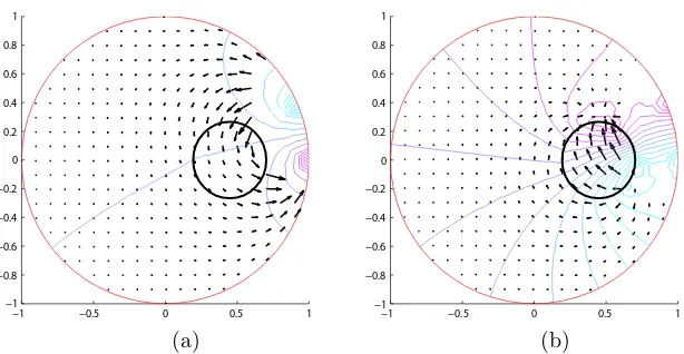
Figure 2. Equipotential lines (solid lines) and electric field streamlines (arrows) of the complex

potentialuωin (1) atω/2π= 100 kHz subject to an injection current between an adjacent pair of electrodes. Complex conductivity values of the anomaly and the background were related to those of banana and saline, respectively. (a) Real part (<{uω}) and (b) imaginary part (={uω}). This figure is quoted from [31].

In fdEIT, we measure the following data setU_ω _{for various angular frequencies:}

U_ω_:= 

      

U1,1

ω −Uω1,2 Uω1,2−Uω1,3 · · · Uω1,L−Uω1,1 U2,1

ω −Uω2,2 Uω2,2−Uω2,3 · · · Uω2,L−Uω2,1

..

. ... ...

..

. ... ...

UL,1

ω −UωL,2 UωL,2−UωL,3 · · · UωL,L−UωL,1



      

← E1yE2 current

← E2yE3 current

.. . .. .

← ELyE1 current

(2)

We try to visualize the change ofγω=σω+iωω due to the change of the angular frequencyω.

If the complex conductivity at two frequencies, γω1, resp.,γω2, is spatially constant in the subject Ω, then

γω1u

j

ω1 =γω2u

j ω2 and

γω2

γω1 =

R

Ωγω1∇u

j ω1· ∇u

k ω1dr

0

R

Ωγω2∇u

j

ω2· ∇ukω2dr

0 =

Uj,k ω1 −U

j,k+1

ω1

Uωj,k2 −U

j,k+1

ω2

This means that we can obtain the quotient γω2

γω1 from the data U_ω

1 and Uω2 without any knowledge of the geometry of Ω or of the electrode positions when the subject is homogeneous.

1.2. Feasibility of fdEIT

For simplicity, we assume that the subject occupies a bounded smooth domain Ω and that it comprises a conductivity anomaly D such that, for each frequency ω, the complex conductivity distribution γω(r) =

γ(r, ω) = σ(r, ω) +iω(r, ω) is constant in the background Ω\D¯, and constant in the anomaly D. The respective constants may change withω.

Assume thatuj

ω is the solutions of (1). Forr∈∂Ω and a sufficiently smalls >0, the complex potentialujω

atrs=r−sn(r) can be expressed as

ujω(rs) =−

Z

Ω

(5)

where Φ(r,r0_{) is the Neumann function of the Laplace operator in the domain Ω. Denoting the background}

conductivity at the angular frequencyωbyαb

ω=γω|Ω\_D¯, we have

ujω(rs) =−

1

αb ω

Z

Ω

γω(r0)∇Φ(rs,r0)· ∇ujω(r0)dr0+

1

αb ω

Z

D

[γω(r0)−αbω]∇Φ(rs,r0)· ∇ujω(r0)dr0.

Usingγω1

∂uj ω1

∂n ≈γω2

∂uj ω2

∂n on∂Ω and takings→0

+_{, we get}

αbω2u

j

ω2(r)−α

b ω1u

j ω1(r)≈

Z

D

∇Φ(r,r0)·

τ2(r0)∇ujω2(r

0₎₋_τ

1(r0)∇ujω1(r

0₎

dr0, r∈∂Ω,

where τl = γωl−αb

ωl, l = 1,2. This approximation provides a relationship between the anomalyD and the

weighted differenceαb

ω2Uω2−α

b

ω1Uω1 in such a way that

αb ω2U

j,k ω2 −α

b ω1U

j,k ω1 ≈

Z

D

∇Φ(rk,r0)·τ2(r0)∇uj_ω₂(r0)−τ1(r0)∇uj_ω₁(r0)dr0, k, j= 1,2, . . . , L,

whererk is the center position of the electrodesEk. Replacing∇ujω by a scalar multiple of∇u j

0, we have

Uωj,k2 −αU

j,k ω1 ≈

Z

D

∇Φ(rk,r0)·βj(r0)∇uj0(r0)

dr0, k= 1,2, . . . , L,

where α = α

b ω1

αb ω2

and we use the rough approximation βj∇uj0 ≈ 1

αb ω2

h

τ2∇ujω2−τ1∇u

j ω1

i

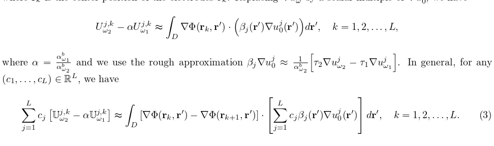
. In general, for any (c1, . . . , cL)∈RL, we have

L

X

j=1

cj Uj,k_ω

2 −αU

j,k ω1 ≈ Z D

[∇Φ(rk,r0)− ∇Φ(rk+1,r0)]·





L

X

j=1

cjβj(r0)∇uj0(r

0₎ 

dr0, k= 1,2, . . . , L. (3)

We may refer to [19] for the above approximation.

The approximation (3) relates the row space of the matrixU_ω

2−αUω1 to the space spanned by the potential differences between adjacent electrodes of electric dipoles,∇Φ(rk,r0)− ∇Φ(rk+1,r0), situated in pointsr0 inside

the anomalyD. This relation is exploited by the factorization method which was introduced by Kirsch [21] for inverse scattering problems and extended to EIT-problems by Br¨uhl and Hanke in [6, 7], see also [12, 22] for further extensions. In the paper [14] we derive the following rigorous range criterion showing the feasibility of the factorization method to fdEIT:

Observation 1.1 ( [14]).

z∈D if and only if ∇Φ(·, z)|∂Ω·d ∈ R

<{αb_ω

2Λω2−α

b ω1Λω1}

1/2

where dis an unit vector, R(A) is the range of the operator A, and Λω is the Neumann-to-Dirichlet operator at the angular frequency ω.

(6)

−1 −0.5 0 0.5 1 −1

−0.8 −0.6 −0.4 −0.2 0 0.2 0.4 0.6 0.8 1

(a) (b) (c)

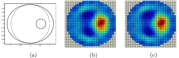
Figure 3. Effect of a boundary geometry error. (a) The ellipse with solid line was the true

imaging domain and the circle in dashed line was the computational model domain. The small disk inside the domain was an anomaly. Complex conductivity values of the anomaly and the background were those of the banana and the saline , respectively. (b) and (c) are reconstructed static images (real-part images) at frequenciesω1

2π = 100 Hz and ω2

2π = 50 kHz, respectively. Each

image was reconstructed using the boundary voltage data from the homogeneous computational model domain as the reference data. This figure is quoted from [31].

−1 −0.5 0 0.5 1

−1 −0.8 −0.6 −0.4 −0.2 0 0.2 0.4 0.6 0.8 1

(a) (b) (c)

Figure 4. Robustness of the proposed fdEIT algorithm against a boundary geometry

er-ror. (a) The same true and computation domains explained in figure 3(a). (b) Real part of the reconstructed frequency-difference image <{αbγω2 −γω1} and (c) imaginary-part image ={αbγω2 −γω1}. Two frequencies were

ω1

2π = 100 Hz and ω2

2π = 50 kHz. The homogeneous

computational model domain was used to compute the sensitivity matrix. This figure is quoted from [31].

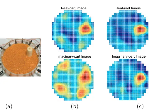
Recently, using a 16-channel multi-frequency EIT (mfEIT) system KHU Mark1, we performed a fdEIT imaging experiment using a phantom with frequency-dependent complex conductivity distribution [18]. The results in [18] show that fdEIT is promising for imaging the complex conductivity contrast of an anomaly such as blood in hemorrhagic stroke and cancer tissue in breast. In [13], we carefully studied the practical implementation of the factorization method for the phantom experiment and justified a discrete version of observation 1.1 by relating it to the localized potentials in [11] that have high energy on some given subset of a domain and low energy on another.

(7)

Real-part Image

Imaginary-part Image

Real-part Image

Imaginary-part Image

(a) (b) (c)

Figure 5. Phantom experiment of a homogeneous background with a frequency-dependent

complex conductivity. (a) Picture of the phantom including banana in the background with packed tiny pieces of carrots. (b) and (c) are reconstructed fdEIT images using the simple differenceU_ω

2−Uω1 and weighted voltage differencesUω2−αUω1, respectively. This figure is quoted from [18]

2. _{Frequency difference TAS}

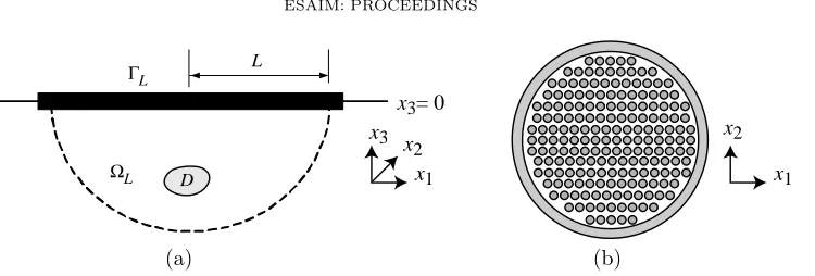
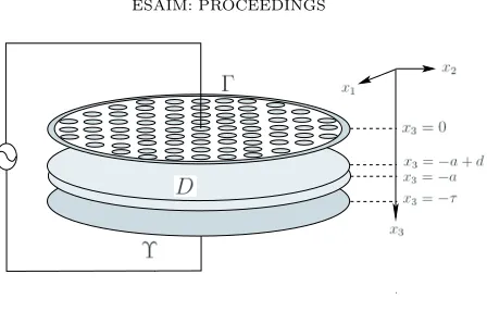
In the paper [19], we apply the fdEIT method to a trans-admittance scanner (TAS), a device for detecting anomalies (such as breast cancer) whose conductivity is significantly different from surrounding tissues of normal conductivity [2, 3, 17, 30, 32]. On the surface of a region of a patient breast, we place a scanning probe with a planar array of electrodes kept at the ground potential and a patient holds a reference electrode with one hand through which a sinusoidal voltage V0sinωt is applied. Let the human body occupy a three-dimensional

domain Ω with a smooth boundary∂Ω. Let Γ andγbe portions of∂Ω, denoting the probe plane placed on the breast and the surface of the metallic reference electrode, respectively. As in the previous section, the resulting electric potential at a positionr= (x, y, z) and timet can be expressed as the real part ofu(r)eiωt where the corresponding complex potentialuω atω satisfies the following mixed boundary value problem:



   

   

∇ ·((σ+iω)∇uω(r)) = 0 in Ω, uω(r) = 0, r∈Γ, uω(r) = V0, r∈γ,

(σ+iω)∇uω(r)·n(r) = 0, r∈∂Ω\(Γ∪γ).

In multi-frequency TAS, we apply the voltage with two different frequenciesf1=ω1/2π andf2 =ω2/2π with

50Hz≤f1< f2≤500kHz and measure two sets of corresponding Neumann datag1=gω1andg2=gω2through Γ at the same time. The inverse problem is to recover the anomaly such as breast cancer from the weighted difference between g1 andg2. In this section, we summarize some results in the paper [19] which provides a

rigorous relation between the anomaly information and the weighted frequency difference. We denote the real and imaginary part ofuωj =uj respectively by<{uj}=vj and={uj}=hj.

(8)

x₃= 0

Γ_L

ΩL D

L

x₁ x2

x3

x₁ x₂

(a) (b)

Figure 6. (a) Simplified model of the breast region with a cancerous lesionD under the scan

probe. (b) Schematic of the scan probe in the (x1, x2)-plane.

conductivity at the angular frequencyωj byγj=σ+iωjj. Assumeγj is a constant inD and in ΩL\D;

σ=

σn in ΩL\D

σc in D and j =

j,n in ΩL\D

j,c inD. (4)

For simplicity, we letz be the axis normal to Γ and let the center of Γ be the origin. Hence, the probe region Γ can be approximated as a two-dimensional region Γ ={(x, y,0) : p

x2₊_y2 _{< L}_}_where_L _{is the radius of the}

scan probe.

The following observation explains an explicit relation betweenD and=(g2−αg1) whereα=σn +iω22,n σn+iω11,n. Observation 2.1( [19]). The imaginary part of the weighted differenceg2−αg1satisfies the following formula:

1

2σn=(g2−αg1)(r) =

Z

D ∇r0

∂Φ(r,r0)

∂z ·Θ(r

0₎_dr0

+ ∂

∂z

Z

∂Ω\Γ

∂Φ(r,r0)

∂z0 Z

D ∇˜rΨ(r

0_,_˜_r₎_·_Θ(˜_r₎_d_˜_r

ds, r∈Γ,

where

Θ(r) = σn−σc

σn ∇(h2−h1)(r) +

ω2(2,n−2,c)

σn ∇(v2−v1)(r)− =(β∇u1(r)), and

β= i 1 +iω11,n

σn

ω22,n σn

₂_,c

2,n − σc

σn

−ω11,n σn

₁_,c

1,n −σc

σn

−iω1ω21,n2,n σ2

n

₁_,c

1,n −2,c

2,n

.

In order to simplify the above representation formula, let us impose the following assumptions

¯

D⊂ΩL/2, D=Bδ(ξ), δ≤dist(D,Γ)≤C1δ,

max

_j,n

j,c, σn σc

≤κ1,

ω22,n σn ≤κ2

σn σc,

σc σn ≤κ3,

where C1 is a positive constant,Bδ a ball with the radius δand the center ξ, _Lδ ≤ ₁₀1,κ1 and κ2 are positive

constants less than 1

2 andκ3is a positive constant less than 10. Taking advantage of these assumption, we have

the following observation.

Observation 2.2( [19]). The imaginary part of the weighted frequency differenceg2−αg1can be expressed as

1

2σn=(g2−αg1) (r) =

Z

D ∂ ∂z

(r−r0)·Θ(˜ r0)

(9)

0.04 0.05 0.06 0.07 0.08 0.04 0.05 0.06 0.07 0.08 −3 −2 −1 0 1 2 3

x 10−4

0.04 0.05 0.06 0.07 0.08 0.04 0.05 0.06 0.07 0.08 −3 −2 −1 0 1 2 3

x 10−4

0.04 0.05 0.06 0.07 0.08 0.04 0.05 0.06 0.07 0.08 −3 −2 −1 0 1 2 3

x 10−4

0.04 0.05 0.06 0.07 0.08 0.04 0.05 0.06 0.07 0.08−1 0 1 2 3 4 5

x 10−4

0.04 0.05 0.06 0.07 0.08 0.04 0.05 0.06 0.07 0.08−3 −2 −1 0 1 2 3

x 10−4

0.04 0.05 0.06 0.07 0.08 0.04 0.05 0.06 0.07 0.08−3 −2 −1 0 1

x 10−4

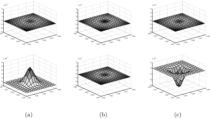
(a) (b) (c)

Figure 7. Frequency-difference trans-admittance map: real and imaginary parts ofg2−αg1

with three different values cases; (a)µ=2,c 2,n −

σc σn

>0 (b)µ= 0 (c)µ <0. We quote this figure from [19].

where

˜

Θ = σn−σc

σn ∇h2− ω22,n

σn ₂_,c 2,n − σc σn

∇v1,

and the error term Error(r)is estimated by

|Error(r)| ≤

ω22,n σn P1

2,c 2,n − σc σn δ3 L3 +

ω11,n σn P1

1,c 1,n − σc σn

+ (ω22,n

σn ) 2_P 2 2,c 2,n − σc σn δ3

|r−ξ|3

.

Here, Pn(λ) is a polynomial function of order n such that Pn(0) = 0 and its coefficients depend only on κj, j= 1,2,3.

In order to test the above observation, we consider a cubic model Ω := [ 0,0.12 ]×[ 0,0.12 ]×[ 0,0.12 ] m3

with the probe region Γ := {(x, y,0.12) : px2₊_y2 _<₀_.₀₃_}_{and the reference electrode} _γ _:=_{₍_{x, y, z}₎_∈ _{Ω :}

z= 0}. Figure 7 shows the images ofg2−αg1 with three different values ofω22,c that are chosen so that the

correspondingµ=2,c 2,n −

σc σn

is positive, zero, or negative, respectively.

3. _{Frequency differential voltage drop method in NDE}

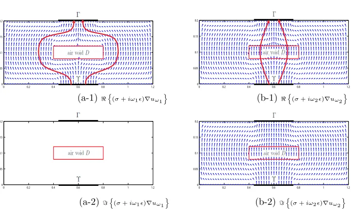
In [20], S. Kimet al.initiated a new remarkable nondestructive evaluation method, called fdEIS (frequency differential electrical impedance scanning), for evaluating the thickness of voids or cracks in conducting ma-terials which is impossible in other conventional nondestructive methods. Finding the location of cracks and voids is relatively easy using any conventional NDE techniques such as ultrasonic testing, impact-echo, radio-graphic testing, electric potential drop method, and so on. However, all existing NDE techniques have inherent limitations in measuring the thickness of the cracks quantitatively.

(10)

Figure 8. 1-D fdEIS Model

the scan probe and the reference electrode are placed, respectively, as in Figure 9. The basic mathematical model of fdEIS is the same as that of fdTAS in the previous section. We apply a sinusoidal voltage of V0sinωt

through Υ with the scan probe Γ kept zero potential and measure the Neumann datagω on Γ with respect to the angular frequency variableω.

In [20] S. Kimet al. found the following interesting relation between the thickness of the cracks and _dωd gω,

the derivative of the Neumann data with respect to angular frequency.

Observation 3.1( [20]). Assumegωis the measured Neumann data corresponding to the 1-D model shown in figure 8. Letω˜=ω0. Then

d

dω˜=gω(0)|ω˜=0 =

V0/d if D6=∅.

0 if D=∅. (5)

This fundamental principle in 1-D fdEIS explains how the frequency mapgω is related with the thickness of the voidD. This interrelation can be described more clearly by introducing theω−distance betweenΓ and Υ defined by

distω(Γ,Υ) = R V0

Γ|gω|ds

.

Figure 9 shows how theω−distance betweenΓandΥ is related with the flow of the current density (σ+iω)∇uω.

4. _Conclusion

Although there have been numerous research outcomes in EIT since early 1980s, the ill-posed nature of the inverse problem in EIT will continue to remain anyway and we should not expect EIT to compete with other medical imaging modalities in terms of spatial resolution. We have no hope in the static EIT without dealing with the forward modeling errors. To alleviate undesirable effects of modelling errors, we suggest fdEIT. The frequency dependent characteristics of biological tissue conductivity and permittivity are not available from any other imaging modality, fdEIT itself can be also quite promising for providing additional diagnostic information. Also, fdEIT method may find applications in various non-destructive evaluations such as crack evaluation, bubble detection, and others.

References

1. G. Alessandrini, V. Isakov, and J. Powell,Local uniqueness in the inverse problem with one measurement, Trans. Amer. Math. Soc.347(1995), 3031–3041.

2. H. Ammari, O. Kwon, J. K. Seo, and E. J. Woo,T-scan electrical impedance imaging system for anomaly detection, SIAM J. Appl. Math.65(2004), 252–266.

(11)

0 0.2 0.4 0.6 0.8 1 1.2 0

0.05 0.1 0.15 0.2

0 0.2 0.4 0.6 0.8 1 1.2 0

0.05 0.1 0.15 0.2

(a-1)<n(σ+iω1)∇uω1 o

(b-1)<n(σ+iω2)∇uω2 o

0 0.2 0.4 0.6 0.8 1 1.2

0 0.05 0.1 0.15 0.2

0 0.2 0.4 0.6 0.8 1 1.2

0 0.05 0.1 0.15 0.2

(a-2)=n(σ+iω1)∇uω1 o

(b-2)=n(σ+iω2)∇uω2 o

Figure 9. The vector fields of real and imaginary parts of (a) (σ+iω1)∇uω1 with

ω1

2π = 10Hz

and (b) (σ+iω2)∇uω2 with

ω2

2π = 10

5_{Hz. The curved arrows in (a-1) and (b-1) mean that the}

electrical current cannot pass through the void at the frequency 10Hz, while it can pass though the void at the higher frequency 105_{Hz. This figure was quoted from [20].}

4. D. C. Barber and B. H. Brown,Applied potential tomography, J. Phys. E. Sci. Instrum.17(1984), 723–733.

5. K. Boone, D. Barber, and B. Brown,Imaging with electricity: report of the european concerted action on impedance tomography, J. Med. Eng. Tech21(1997), 201–232.

6. M. Br¨uhl,Explicit characterization of inclusions in electrical impedance tomography, SIAM J. Math. Anal.32(2001), 1327– 1341.

7. M. Br¨uhl and M. Hanke,Numerical implementation of two non-iterative methods for locating inclusions by impedance tomog-raphy, Inverse Problems16(2000), 1029–1042.

8. M. Cheney, D. Isaacson, and J. C. Newell,Electrical impedance tomography, SIAM Review41(1999), 85–101.

9. M. Cheney, D. Isaacson, J. C. Newell, S. Simske, and J. Goble, Noser: An algorithm for solving the inverse conductivity problem, Int. J. Imaging Sys. and Tech.2(1990), 66–75.

10. A. Friedman and V. Isakov,On the uniqueness in the inverse conductivity problem with one measurement, Indiana Univ. Math. J.38(1989), 553–580.

11. B. Gebauer,Localized potentials in electrical impedance tomography, Inverse Probl. Imaging2(2008), 251–269. 12. M. Hanke and M. Br¨uhl,Recent progress in electrical impedance tomography, Inverse Problems19(2003), S65–S90. 13. B. Harrach and J. K. Seo,Anomaly detection with frequency-difference electrical impedance tomography, preprint.

14. ,Detecting inclusions in electrical impedance tomography without reference measurements, SIAM J. Appl. Math. (sub-mitted) (2009).

15. D. Holder,Electrical impedance tomography: Methods, history and applications, Bristol, UK, IOP Publishing (2005). 16. V. Isakov,On uniqueness of recovery of a discontinuous conductivity coefficient, Comm. Pure Appl. Math.41(1988), 856–877. 17. J. Jossinet and M. Schmitt, A review of parameters for the bioelectrical characterization of breast tissue, Ann. New York

Academy of Sci.873(1999), 30–41.

18. S. C. Jun, J. Kuen, J. Lee, E. J. Woo, D. Holder, and J. K. Seo,Frequency-difference EIT (fdEIT) using weighted frequency difference and equivalent homogeneous complex conductivity: phantom imaging experiments, preprint.

19. S. Kim, J. Lee, J. K. Seo, E. J. Woo, and H. Zribi,Multi-frequency trans-admittance scanner: mathematical framework and feasibility, SIAM J. Appl. Math. (to appear).

20. S. Kim, J. K. Seo, and T. Ha,A nondestructive evaluation method of concrete voids: frequency differential electrical impedance scanning, SIAM J. Appl. Math. (submitted).

21. A. Kirsch, Characterization of the shape of a scattering obstacle using the spectral data of the far field operator, Inverse Problems14(1998), 1489–1512.

22. ,he factorization method for a class of inverse elliptic problems, Math. Nachr278(2005), 258–277.

(12)

24. P. Metherall,Three dimensional electrical impedance tomography of the human thorax, University of Sheffield, Dept. of Med. Phys and Clin. Eng., 1998.

25. P. Metherall, D. C. Barber, R. H. Smallwood, and B. H. Brow,Three-dimensional electrical impedance tomography, Nature 380(1996), 509–512.

26. A. Nachman,Reconstructions from boundary measurements, Ann. Math.128(1988), 531–576.

27. ,Global uniqueness for a two-dimensional inverse boundary value problem, Ann. Math.142(1996), 71–96.

28. T. I. Oh, W. Koo, K. H. Lee, S. M. Kim, J. Lee, S. W. Kim, J. K. Seo, and E. J. Woo,Validation of a multi-frequency electrical impedance tomography (mfEIT) system KHU Mark1: impedance spectroscopy and time difference imaging, Physiol. Meas.29 (2008), 295–307.

29. G. J. Saulnier, R. S. Blue, J. C. Newell, D. Isaacson, and P. M. Edic,Electrical impedance tomography, IEEE Sig. Proc. Mag. 18(2001), 31–43.

30. J. K. Seo, O. Kwon, H. Ammari, and E. J. Woo,Mathematical framework and anomaly estimation algorithm for breast cancer detection: electrical impedance technique using ts2000 configuration, IEEE Trans. Biomed. Eng.51(2004), 1298–1906. 31. J. K. Seo, J. Lee, H. Zribi, S. W. Kim, and E. J. Woo,Frequency-difference electrical impedance tomography (fdeit): Algorithm

development and feasibility study, Physiol. Meas.29(2008), 929–944.

32. J. E. Silva, J. P. Marques, and J. Jossinet,Classification of breast tissue by electrical impedance spectroscopy, Med. Biol. Eng. Comput.38(2000), 26–30.

33. E. Somersalo, M. Cheney, and D. Isaacson, Existence and uniqueness for electrode models for electric current computed tomography, SIAM J. Appl. Math.22(1992), 1023–40.

34. J. Sylvester and G. Uhlmann,A uniqueness theorem for an inverse boundary value problem in electrical prospection, Comm. Pure Appl. Math.39(1986), 91–112.

35. ,A global uniqueness theorem for an inverse boundary value problem, Ann. Math.125(1987), 153–169.

36. G. Uhlmann,Developments in inverse problems since calderdon’s foundational paper, Harmonic analysis and partial differential equations (Chicago, IL, 1996), Univ. Chicago Press (1999), 295–345.