M. Ismail, B. Maury & J.-F. Gerbeau, Editors
A STOKESIAN SUBMARINE
Aline Lefebvre-Lepot
1and Benoˆ
ıt Merlet
2Abstract. We consider the problem of swimming at low Reynolds numbers. This is the relevant asymptotic for micro- and nano-robots needing to navigate in an aqueous medium. As a model, we propose a robot composed of three balls. The relative positions of these balls can change according to three degrees of freedom. We prove that this robot is able to navigate in a plane by modifying the conformation of its shape.
R´esum´e. Nous consid´erons le probl`eme de la nage `a faible nombre de Reynolds. C’est l’asymptotique pertinente pour les micro- et nano-robots devant se d´eplacer dans un milieu aqueux. Nous proposons comme mod`ele un robot form´e de trois boules qui peuvent se d´eplacer les unes par rapport aux autres selon trois degr´es de libert´e. Nous d´emontrons qu’en changeant sa conformation, ce robot peut effec-tivement naviguer dans un plan.
1.
Introduction
In this note we are concerned with the problem of self-propulsion at low Reynolds numbers. Namely, is it possible for a swimmer submerged in a Stokes fluid to move solely by changing the configuration of its shape ? Recent studies have shown that a solid can swim by prescribing the velocity of the fluid on its surface, see [10]. Here we assume that the velocities of the fluid and of the swimmer are equal on its boundary.
Swimming at low Reynolds numbers is the problem faced by microorganisms such as bacteria, unicellular eukaryotes or special cells of multicellular organisms such as sperm cells. A lot of papers are dedicated to this subject in the biological literature. We refer to the recent paper [6] for a description of known biological swimming mechanisms and an overview of the subject.
From the physicist’s point of view, the subject has been initiated by Taylor [14], Lighthill [7] and later Purcell [9] and Shapere and Wilczek [12, 13]. The motion of a micro-swimmer is dominated by viscosity and inertia is negligible. In this situation, it turns out that the instantaneous global displacement of the swimmer is a linear function of its deformation. In particular, the total displacement of the swimmer only depends on the assumed sequence of shapes and not on the velocity this sequence has been ran through. Moreover a reciprocal deformation does not lead to any displacement and then at low Reynolds numbers, an efficient swimmer has to perform non-reciprocal strokes. Consequently, at small scales, swimming is not an obvious task. However some model swimmers, being able to move along a line, have been proposed [4, 8, 9].
The swimming issue is not only theoretical. Low Reynolds numbers are also the right asymptotic regime for swimming micro- or nano-robots. In the near future we can imagine building some micro-devices that navigate and interact with biological systems. Very recently, a 250 µm-length micro-motor has been designed [15]
1 CMAP (Centre de Math´ematiques Appliqu´ees) Ecole Polytechnique, route de Saclay 91128 Palaiseau Cedex, France, [email protected]
2Universit´e Paris Nord - Institut Galil´ee LAGA (Laboratoire d’Analyse, G´eom´etrie et Applications) Avenue J.B. Cl´ement 93430 Villetaneuse, France, [email protected]
c
EDP Sciences, SMAI 2009
opening the possibility for practical micro-surgeons. In this direction it is interesting to study simple devices that are able not only to translate but also to navigate. By navigating we mean translating and rotating.
We will introduce below such a model robot composed of three coplanar spheres and prove its ability to navigate in a plane. The proof is similar to the one proposed in [2] in the sense that the question of whether the device is able to navigate reduces to a controllability problem. As in [2], local controllability is obtained for large values of the control parameters. However, here we deal with 3 control parameters and 2D displacements rather than 2 control parameters and 1D displacements. Moreover, the asymptotic analysis has been drastically simplified and now allows to consider devices made of an arbitrary number of spheres.
In the rest of this introduction, we set the swimming problem, briefly describe existing micro-swimmers and finally present our model and main result.
Swimming at low Reynolds numbers
At small scales and small velocities, inertia is negligible compared to viscosity. If Kis the region filled by a swimmer and Γ =∂K its boundary, we can assume that the velocity and pressurev, pin the surrounding fluid solve the Stokes equations:
−η∆u+∇p = 0 inR3\K,
∇ ·u = 0 inR3\K, u = g on Γ, u, p → 0 at∞
(1.1)
The boundary velocitygis the sum of a contribution due to the deformation of the swimmer and of a contribution due to the rigid induced displacement. Let us describe these contributions and introduce some notations.
As noticed in [11], since we neglect inertia, there is no canonical way to attach a center and a set of axes to the swimmer. We have to choose arbitrarily a standard position and an orientation for each shape. In the sequel we only consider families of shapes characterized by a finite number of parameters l = (l1,· · ·, ln)
varying in an open setL ⊂Rn. The standard positions of the shapes we consider are given by a family (γl) of homeomorphisms:
γl : Γ −→Γl,
where Γ is a reference shape. The position xof a point of the boundary is then given by
x = c+θγl(x0),
wherex0is a point of the fixed reference shape Γ and (c, θ)∈R3×SO3(R) characterize the solid displacement.
Next, the velocity of the boundary at this point writes
g(x) = v+ω×x+θw(x), (1.2)
wherev, ω∈R3are the instantaneous speed and rotation of the solid referential and wherew = ( ˙l· ∇)γl(x0)
corresponds to the velocity due to the deformation of the swimmer.
The surface density of the forces applied by the swimmer on the fluid on Γl is given by the formulaf(x) = σ(x)n(x), whereσ:=η(∇u+∇ut)−pIdis the Cauchy stress tensor in the fluid,nis the inner unit normal to
K on Γl and (u, p) solve (1.1) with boundary data (1.2). If no external force is applied on the fluid-swimmer system, neglecting inertia, the total force and torque exerted by the swimmer on the fluid must vanish. We obtain the following system of six conditions
Z
Γl
σn(x)dx = 0,
Z
Γl
x×σn(x)dx = 0. (1.3)
Solving these equations we obtain the instantaneous solid displacement as a linear function of ˙l:
Notice that the coefficients depend non-linearly on the shape parameterl.
We will call stroke any closed path{l(t), t∈[0, T]}in the set of parameters and say that our robot is able to swim if there exists a stroke leading to a non-vanishing net displacementc(T)−c(0) = R0Tv.
A well known result called the Scallop Theorem (see e.g. [2,6,9,13,14]) states that a stroke in a one parameter family of shapes does not lead to any displacement. Indeed, in such a case, we may write
Z T
0
v = Z T
0
Gl1(s)l˙1(s)ds = I
Gl1dl1 = 0.
Examples of swimmers
Swimming at low Reynolds number is thus very far from the intuition we usually develop at our scales. Anyway, there exist some model robots which are known to be able to swim. We briefly describe three of them. Each one corresponds to a two-parameter family of shapes.
l1
l2
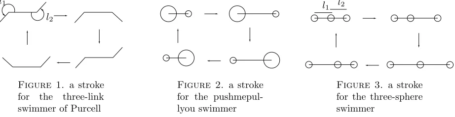
Figure 1. a stroke for the three-link swimmer of Purcell
Figure 2. a stroke for the pushmepul-lyou swimmer
l1 l2
Figure 3. a stroke for the three-sphere swimmer
The first one was proposed by Purcell [9]. It is an object composed of three solid lines linked by two hinges. The two shape parameters are the anglesl1andl2between two consecutive lines. By varying alternatively these
angles we obtain the non-reciprocal stroke shown Fig. 1. In that case, the scallop Theorem does not apply and this stroke can lead to a net displacement along the horizontal axis.
As a second example, we present the pushmepullyou swimmer of Avron, Kenneth and Oakim [4]. It is made of the union of two spheresS1, S2. The two parameters are the distance between the centers of the spheres and
the ratio between their volume, the total volume being fixed — see Fig. 2.
Our last example is the three-sphere swimmer of Najafi and Golestanian [8]. The robot is composed of three identical aligned spheres. The shape parameters are the distances between two consecutive spheres — see Fig. 3.
These three robots are known to be able to swim — see [2, 4, 8].
In these examples, we obtain a displacement along one direction. Let us now introduce a new simple robot being able to navigate (translate and rotate) in a plane.
A three-ball submarine
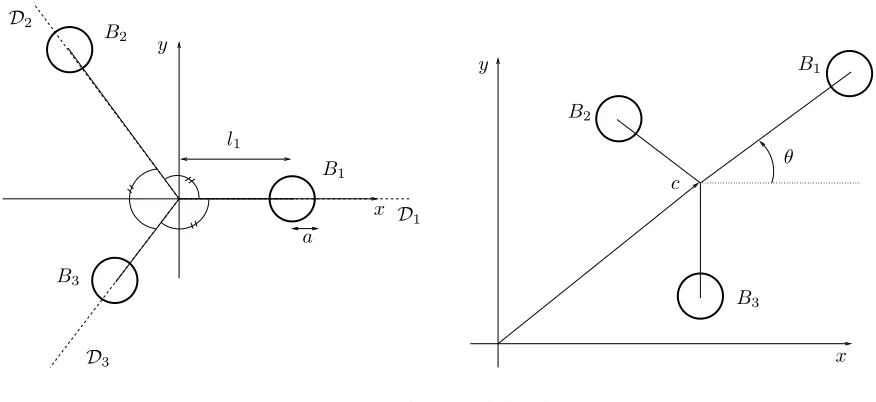
Our robot is composed of three ballsB1, B2, B3 of radiia >0. The structure of the robot is built on three
raysD1,D2,D3 ⊂ {z= 0} spanned by the three vertices of an equilateral triangle centered at 0 — see Fig. 4.
Fori= 1,2,3, the center of the ballBi can translate freely along the rayDi but we assume that the balls do not rotate in the frame attached to D1,D2,D3. As a consequence, the shape of the robot is characterized by
the three distancesl1, l2, l3 between the centers of the balls and the origin.
Of course, by symmetry, this robot can not move in the z direction. For the same reason, it can not rotate around a non-vertical axis. The state of the three-ball submarine is determined by the three lengths l1, l2, l3,
the coordinates c1, c2 of the intersection of D1,D2,D3 and the algebraic angle θ between ex and D1. In this
particular case, we may rewrite (1.4) as
˙
B1
B3
B2
D1
D3
D2
l1
a y
x
B1
B3
B2
y
x c
θ
Figure 4. The three-ball submarine
WritingX = (l, c, θ), the evolution of the state of the submarine is given by the relation
˙
X = FXl˙ := ( ˙l, VXl,˙ ΩXl˙). (1.5)
Our main result states that if the parameters are allowed to vary in the neighborhood of{l1=l2=l3= 1/ε}
withε >0 small enough, then the three-ball submarine can achieve any small displacement in the plane.
Theorem 1.1. For ε > 0 small enough, there exists a neighborhood N of Xε := ((1/ε,1/ε,1/ε),0,0,0) in (0,+∞)3
×R2×R such that for anyXi, Xf ∈ N, there exists a solution to (1.5)with end points Xi, Xf. By translation and rotation invariance of the problem, we see that repeating small strokes, our submarine can achieve any translation and any rotation in the plane.
A controllability problem
Following the method of [2], we rephrase Theorem 1.1 in the language of control theory. In this setting, Theorem 1.1 claims that system (1.5) is locally controllable atXεforεsmall enough.
LetF1
X, FX2, FX3 denote the rows of the matrixFX, i.e: FXi :=FXei where (e1, e2, e3) is the canonical basis
of R3. Let [Fi X, F
j
X] denotes the Lie bracket (FXi · ∇)F j X −(F
j
X · ∇)FXi. Chow’s Theorem gives a sufficient condition for local controllability (see e.g. [1]) is:
spanDFX1ε, F
2
Xε, F
3
Xε, [F
i X, F
j
X]|X=Xε,1≤i < j ≤3 E
= R3×R2×R. (1.6) WritingFk
X= (ek, TXk), withTXk := (VXk,ΩkX)∈R3, we easily compute that this condition is equivalent to det (FX1 · ∇)TX2 −(FX2 · ∇)TX1, (FX2 · ∇)TX3 −(FX3 · ∇)TX2, (FX3 · ∇)TX1 −(FX1 · ∇)TX3
|X=Xε 6= 0. (1.7)
Remark 1.2. IfD1,D2,D3 are not assumed to be coplanar, we expect that any solid displacement inR3 can
be achieved (and not only planar displacements). In that case we should add iterated Lie brackets of the form [Fi
X,[F j
X, FXk]] in condition (1.6).
In Section 2 we briefly recall well known results on the Stokes problem (1.1) in the complement ofn balls. We also establish an asymptotic result for this Stokes problem in the regime of large distances between balls. In Section 3 we prove Theorem 1.1
2.
Stokes Problem in the complement of
n
balls
In this section, we consider the Stokes problem in the complement ofnballs of radiia >0.
In the sequelB is the closed ball of radiusa centered at 0 andBy :=y+B denotes the ball centered at a point y∈R3. A configuration ofnballs is characterized by their centers x= (x1,· · · , xn)∈(R3)n. We only
consider configurations of non-overlapping balls by imposingx∈ Cn where
Cn := y∈(R3)n : R(y)>2a , with R(y) := min
i6=j |yi−yj|.
We now fixx∈ Cn. The domain filled by the fluid is Ωx:=R3\(∪1≤i≤nBxi). Let us introduce the Hilbert
spaceH1/2:=H1/2(∂B,R3) and its dual
H−1/2:=H−1/2(∂B,R3). We also define the Cartesian products
Hn1/2 := {g= (g1,· · ·, gn) : gi∈ H1/2}, Hn−1/2 := {f = (f1,· · · , fn) : fi∈ H−1/2}.
Letg∈ H1n/2, the Stokes problem in Ωx, with Dirichlet datagi on∂Bi reads
−η∆u+∇p = 0, in Ωx,
∇ ·u = 0 in Ωx,
u = gi(· −xi) on∂Bxi, fori= 1,· · · , n,
u, p → 0 at ∞
(2.1)
It is well known (see e.g. [5] p. 154) that Problem (2.1) admits a unique solution (u, p)∈ Vx×L2(Ωx) where
Vx := (
v∈ D′(Ωx,R3) : ∇v, p v
1 +|r|2∈L 2(Ωx)
)
.
Moreover we haveσ·n∈H−1/2(∂Ωx,R3) where σ:=η(∇u+∇ut)−pId is the Cauchy stress tensor, andn is the outer unit normal to∂Ωx. From this, fori= 1,· · ·, nwe can definefi∈ H−1/2byfi:={σ·n}(xi+·). We have thus defined a bounded linear application
Φx : g∈ H1/2
n 7−→ f ∈ H−n1/2 (2.2)
associating to a velocity data on the boundary of the balls the resulting surface force density applied by the balls on the fluid. This application is usually called the Dirichlet to Neumann map (for the Stokes problem).
It turns out that the inverse problem is easier since we have an explicit formula for the velocity fielduas a convolution off with the fundamental solution of Stokes equation:
u(r) = n X
i=1 Z
∂Bi
fi(r′−xi)G(r−r′)dr′, with G(r) := 1 8πη
1
|r|+
r⊗r
|r|3 !
. (2.3)
The integrals in the formula have a meaning forr∈Ωxandf ∈ Hn−1/2through the duality productH1/2−H−1/2. On the boundary of the ballBi, this formula leads to
gi(r) = Φ−01fi(r) + X
j6=i Z
∂B
where Φ0 is the application defined by (2.2) in the case n = 1 — notice that by translation invariance this
application does not depend on the position of the ball.
Large distances approximation
For later use we are interested in the asymptotic behavior of Φxand∇xΦx asR(x) := min
i<j |xi−xj|tends to infinity. Let us introduce the notations
xi,j := xi− xj, ri,j := |xi,j| and ei,j := xi,j ri,j.
We first prove
Proposition 2.1. For every f ∈ H−n1/2, we have
(Φ−x1f)i = Φ−01fi+ 1 8πη
X
j6=i 1 ri,j
(Id+ei,j⊗ei,j) Z
∂B
fj+ψx,if,
with kψxkL(H−1/2
n ,H
1/2
n ) . R
−2(x), and
k∇xψxkL(H−1/2
n ,H
1/2
n )3n . R
−3(x).
Proof. Letx∈ Cn andf ∈ Hn−1/2. From (2.2) (2.4) we have fori= 1,· · ·, nandr∈∂B,
(Φ−x1f)i(r) = Φ−01fi(r) + X
j6=i Z
∂B
fi(r′)G(r−r′+xij)dr′. (2.5)
Using the expansion G(xi,j+z) =G(xi,j) +{G(xi,j+z)−G(xi,j)}, for|z| ≤2a, we get
G(xi,j+z) =G(xi,j) + ˜G(xi,j, z) (2.6)
where the functions r2
i,jG˜(xi,j,·) andr3i,j∇xG˜(xi,j,·) remain bounded in anyCk(2B) asri,j tends to infinity.
Plugging (2.6) in (2.5) yields the Proposition.
Since the operator f ∈ Hn−1/2 7→ (Φ0−1f1,· · ·,Φ−01fn) ∈ H 1/2
n is an isomorphism, we deduce the following asymptotic expansion for Φx.
Proposition 2.2. For every g∈ H1n/2,
(Φxg)i = Φ0
gi− 1 8πη
X
j6=i 1 ri,j
(Id+ei,j⊗ei,j) Z
∂B Φ0gj
+φx,ig,
with kφxkL(H1/2
n ,H−
1/2
n ) . R
−2(x), and
k∇xφxkL(H1/2
n ,H−
1/2
n )3n . R
−3(x).
Rigid motion of
n
independent balls in a Stokes fluid
We consider Problem (2.1) with a boundary data g= (g1,· · · , gn) generated by independent rigid motions
of thenballs, i.e, there existsv= (v1,· · ·, vn) andω= (ω1,· · ·, ωn) in (R3)n such that
gi(r) = vi+ωi×r, for i= 1,· · · , n, r∈∂B. (2.7)
We are interested in the force field f = (f1,· · ·, fn) generated by these velocities on the boundaries of
In the casen= 1, the solution is well known: we have
Φ0g1(r) =
η a
3
2v1+ 3ω1×r !
.
Using this formula and Proposition 2.2, we end with
Proposition 2.3. Let x∈ Cn andg of the form (2.7), we have
(Φxg)i = 3 2 η a
vi+ 2ωi×r− 3 4
X
j6=i a ri,j
(vj+ (ei,j·vj)ei,j)
+ϕx,i(v, ω),
with kϕx(v, ω)k H−1/2
n . R
−2(x)
|v, ω|, and k∇xϕx(v, ω)kH−1/2
n . R
−3(x)
|v, ω|.
Notice that sinceR∂Bω×r dr= 0, rotations do not appear in theO(R−1(x)) terms of the asymptotic.
3.
Local controllability of the three-ball submarine
In this section we prove Theorem 1.1: the three ball submarine is locally controllable in the neighborhood of l = (1/ε,1/ε,1/ε). We have seen that it were sufficient to establish (1.7). To do so, in the following, we write the self propulsion conditions (1.3) for Xε = ((1/ε,1/ε,1/ε),0,0,0). Then using Proposition 2.3 we compute the leading order of Fi
Xε as εtends to 0.
Next, using again Proposition 2.3 and conditions (1.3), we find the leading order term of (FXi · ∇)T j X at X =Xε.
Finally, we compute the leading order of the determinant in equation (1.7) and conclude.
Conventions and Notations
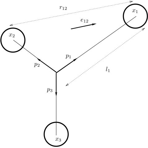
First we introduce some notations in order to describe the motion of the three ball submarine. Fori= 1,2,3, letxi be the center of the ball Bi andpi the unit vector
pi :=
xi−c
|xi−c| .
By symmetry the points xi and c remain in the plane{z = 0}. In the sequel we identify R2 with the plane
{z= 0} ⊂R3and we consider thatxi, candpi are 2-dimensional vectors. Forx= (x1, x2)∈R2, we will write x⊥ := (−x2, x1)
to denote theπ/2-rotation ofx.
The positionxi may be written
xi = c+lipi
The velocity of ballBi results from the rigid motion of the frame attached to (c, p1, p⊥1)⊂ {z = 0} and from
the translation of the ball in this frame. The instantaneous motion of the solid frame is characterized by the velocityv of the centerc and by an angular velocityω∈R. With these notations the velocity ofxi writes
˙
Since the motion ofBxi in the frame (c, p1, p⊥1) is a pure translation in the direction pi, the fluid velocity on
∂Bxi is constrained to be equal to
gi(r) = v+ω(lipi+r)⊥
| {z }
+ ˙lipi |{z}
, r∈∂B, i= 1,2,3, (3.1)
=: hi(v, ω)(r) =:ki(r)
where k stands for the velocity of the point attached to the solid frame andh for the relative velocity of the balls in this frame.
In order to achieve the computations below we introduce the unit vectorsei,j :=
xi−xj
|xi−xj|and the distances ri,j:=|xi−xj|.
x1
x2
x3
l1
r12
p1
p2
p3
e12
Figure 5. Notations for the three-ball submarine
Finally, since we are interested in the regime of large distances between the balls, we perform the change of variables
λ := εl, ρi,j := εri,j, ˜v := εv. (3.2)
Self propulsion
We now write the self propulsion conditions (1.3). By symmetry the vertical component of the total force exerted on the fluid and the horizontal components of the torque vanish so we only keep three conditions:
ei·
3 X
i=1 Z
∂Bi
σn = 0, fori= 1,2 and e3· 3 X
i=1 Z
∂Bi
The forces exerted on the fluid on ∂Bi are given by σn = (Φxg)i = (Φxh)i+ (Φxk)i. Using the asymptotic given in proposition 2.3, we have
(Φxh)i = 3 2 η a
v+ωlip⊥i + 2ωr⊥− 3 4
X
j,j6=i a ri,j
(v+ωljp⊥j) + (ei,j·(v+ωljp⊥j))ei,j
+sx,i((v+ωljp⊥j)j, ω),
(Φxk)i = 3 2 η a
l˙ipi− 3 4
X
j,j6=i a ri,j
˙
lj(pj+ (ei,j·pj)ei,j)
+tx,i(( ˙ljpj)j),
wheresx,1,· · ·, sx,3,tx,1,· · · , tx,3 are linear operators with values inH−n1/2satisfying
ksxk . R−2(x), k∇xsxk . R−3(x) and ktxk . R−2(x), k∇xtxk . R−3(x).
Using the change of variable (3.2), we get
(Φxh)i = 3η 2aε
v˜+ωλip⊥i + 2εωr⊥− 3 4aε
X
j,j6=i 1 ρi,j
(˜v+ωλjp⊥j) + (ei,j·(˜v+ωljp⊥j))ei,j
+εαε,λ,θ(˜v, ω),
(Φxk)i = 3η 2aε
λ˙ipi− 3 4aε
X
j,j6=i ˙ λj ρi,j
(pj+ (ei,j·pj)ei,j)
+εβε,λ,θl˙,
with as ε↓0,
kαx,λ,θkH−1/2, k∇λαx,λ,θkH−1/2, kβx,λ,θkH−1/2, k∇λβx,λ,θkH−1/2 = O(1). Plugging these formulas in (3.3), we obtain the conditions
3˜v+
3 X
i=1
λip⊥i !
ω−34aε
X
i,j, i6=j 1 ρi,j
(Id+ei,j⊗ei,j)
˜v−3 4aε
X
i,j, i6=j 1 ρi,j
λj(p⊥j + (p⊥j ·ei,j)ei,j)
ω
+ε2αfε,λ,θ(˜v, ω) = −
3 X
i=1
˙ λipi+
3 4aε
X
i,j, i6=j ˙ λj ρi,j
(pj+ (pj·ei,j)ei,j) +ε2βε,λ,θf λ,˙ (3.4)
3 X
i=1
λip⊥i ! ˜ v+ 3 X i=1 λ2 i !
ω+εαt
ε,λ,θ(˜v, ω) = εβε,λ,θt λ,˙ (3.5)
with αfx,λ,θ, αt x,λ,θ, β
f
x,λ,θ, βtx,λ,θ, = O(1) and ∇λα f
x,λ,θ, ∇λαtx,λ,θ, ∇λβ f
x,λ,θ, ∇λβx,λ,θt = O(1).
To obtain (3.4) and (3.5) we used the identities pi·pi= 1,pi⊥·pi = 0 andR∂Br = 0. Note that in (3.5) we only keep the leading order terms: it is not necessary to keep track ofO(ε) terms in the computations below.
Proof of
(1.7)
We have seen in the introduction that, by linearity, the global displacement takes the form (1.4) which reads here
˜
In the special caseλ=λ := (1,1,1), the problem is invariant by the three reflections with respect toD1,D2
andD3. As a consequence, we necessarily haveω= 0 and ˜v=κPiλ˙ipi for someκ∈R. Solving (3.4), we get
˜
v = (1 +O(ε)) (
−13
3 X
i=1
˙ λipi
)
, ω = 0.
From this we obtain, fori= 1,2,3, Fiλ
ε,c,θ
= ei,− pi
3 +O(ε),0
. (3.7)
The next step is to compute the brackets(Fk
X· ∇)TXl −(FXl · ∇)TXk |
λ=λ fork6=l. Let us fix 1≤k, l≤3
withk6=l. By translation invarianceTl
X does not depend onc, so, taking into account (3.7), we have
(FXk · ∇)TXl |
λ=λ = ε
∂ ∂λk
TXl|λ=λ =
∂ ∂λk
(˜v, εω)|λ=λ =: ( ˜V , εW), (3.8)
where ˜v,ω solve (3.4)(3.5). Differentiating (3.4) with respect toλk and using (3.7) we obtain
(3Id+O(ε)) ˜V
= 3 4aε ∂ ∂λk X
i,j, i6=j 1 ρi,j
(Id+ei,j⊗ei,j) − pl 3 ! +3 4aε ∂ ∂λk X
j,j6=l 1 ρl,j
(pl+ (pl·el,j)el,j)
+O(ε2). (3.9)
In particular, we used the identitiesP3i=1λip⊥i = P
i6=jλjp⊥j = P
i6=jλj(p⊥j ·ei,j)ei,j = 0 forλ=λ.
Since the unknownW does not appear in this system, we can solve it and obtain ˜V at leading order. After straightforward calculations (postponed to the Appendix below) we conclude:
˜ V = aε
√
3
2432(−9pl−19pk) +O(ε
2). (3.10)
Similarly, differentiating (3.5) with respect toλk, we easily obtain
W = 1 9p
⊥
k ·pl+O(ε). (3.11)
Finally (3.10)(3.11) together with (3.8) yield
(FXk · ∇)TXl −(FXl · ∇)TXk |
λ=λ = ε a
5√3
2332(pl−pk),
2 9p
⊥ k ·pl
!
+O(ε2)
and
det (FX1 · ∇)TX2 −(FX2 · ∇)TX1, (FX2 · ∇)TX3 −(FX3 · ∇)TX2, (FX3 · ∇)TX1 −(FX1 · ∇)TX3
|X=Xε
= −5
2a2ε3
2535 det
p1−p2 p2−p3 p3−p1
p⊥
1 ·p2 p⊥2 ·p3 p⊥3 ·p1
+O(ε4) = −5
2a2ε3
2733 +O(ε 4).
This implies that the determinant does not vanish forεsmall enough, ending the proof of (1.7) and Theorem 1.1.
References
[1] Andrei A. Agrachev and Yuri L. Sachkov.Control theory from the geometric viewpoint, volume 87 ofEncyclopaedia of Math-ematical Sciences. Springer-Verlag, Berlin, 2004. Control Theory and Optimization, II.
[2] Fran¸cois Alouges, Antonio DeSimone, and Aline Lefebvre. Optimal strokes for low Reynolds number swimmers: an example.
J. Nonlinear Sci., 18(3):277–302, 2008.
[3] J.E. Avron, 0. Gat, and O. Kenneth. Optimal swimming at low Reynolds numbers. arXiv (electronic) http://arxiv.org/pdf/math-ph/0404044, pages 1–11, 2008.
[4] J.E. Avron, O. Kenneth, and D.H. Oakmin. Pushmepullyou: An efficient micro-swimmer.New J. Phys., 7:234–238, 2005. [5] Robert Dautray and Jacques-Louis Lions.Mathematical analysis and numerical methods for science and technology. Vol. 4.
Springer-Verlag, Berlin, 1990. Integral equations and numerical methods, With the collaboration of Michel Artola, Philippe B´enilan, Michel Bernadou, Michel Cessenat, Jean-Claude N´ed´elec, Jacques Planchard and Bruno Scheurer, Translated from the French by John C. Amson.
[6] E Lauga and T. Powers. The hydrodynamic of swimming microorganisms.arXiv (electronic) http://arxiv.org/pdf/0812.2887v1, pages 1–48, 2008.
[7] M. J. Lighthill. On the squirming motion of nearly spherical deformable bodies through liquids at very small Reynolds numbers.
Comm. Pure Appl. Math., 5:109–118, 1952.
[8] A. Najafi and R. Golestanian. Simple swimmer at low Reynolds numbers: Three linked spheres. Phys. Rev. E, 69:062901– 062904, 2004.
[9] E.M. Purcell. Life at low Reynolds numbers.Am. J. Phys., 45:3–11, 1977.
[10] Jorge San Mart´ın, Tak´eo Takahashi, and Marius Tucsnak. A control theoretic approach to the swimming of microscopic organisms.Quart. Appl. Math., 65(3):405–424, 2007.
[11] Alfred Shapere and Franck Wilczek. Self-propulsion at low Reynolds numbers.Phys. Rev. Lett., 58:2051–2054, 1987. [12] Alfred Shapere and Frank Wilczek. Efficiencies of self-propulsion at low Reynolds number.J. Fluid Mech., 198:587–599, 1989. [13] Alfred Shapere and Frank Wilczek. Geometry of self-propulsion at low Reynolds number.J. Fluid Mech., 198:557–585, 1989. [14] Geoffrey Taylor. Analysis of the swimming of microscopic organisms.Proc. Roy. Soc. London. Ser. A., 209:447–461, 1951. [15] B. Watson, J. Friend, and L. Yeo. Piezoelectric ultrasonic resonant motor with stator diameter less than 250
µm: the Proteus motor. Journal of Micromechanics and Microengineering, (http://www.iop.org/EJ/article/0960-1317/19/2/022001/jmm9 2 022001.pdf ), 19:1–5, 2009.
A.
Appendix
Starting from (3.9) we exhibit here the computations leading to (3.10). We have to compute forλ=λthe quantities
I := ∂ ∂λk
X
i,j, i6=j 1 ρi,j
(Id+ei,j⊗ei,j)
−
pl 3
!
and II := ∂ ∂λk
X
j,j6=l 1 ρl,j
(pl+ (pl·el,j)el,j)
.
We start by some intermediate identities. Recall that by definition,ρi,j=|λipi−λjpj|and sincepi=−12pj± √
3
2 p⊥j, we haveρi,j= q
(λj+λ2i)2+34λ2i. So forλ=λ,
ρi,j =
√
3, ∂
∂λk
ρi,j = 0 if i6=, j6=k,
∂ ∂λk
ρi,j =
√
3
2 if i=k or j=k.
Next by definition, we have fori6=j, ei,j=ρi,j1 (λipi−λjpj). Thus for λ=λ,
∂ ∂λk
ek,j = 1
2√3(pj+pk), leading to
∂ ∂λk
(ek,j⊗ek,j) = 1
3(pk⊗pk−pj⊗pj).
We will also need the equalities
pl·ek,j = 0 if j=6 l, pl·ek,l=−
√
3
Using these identities we compute
I = 2 ∂ ∂λk
X
j, j6=k 1 ρk,j
(Id+ek,j⊗ek,j)
−
pl 3
!
=
√
3
322(−pl−7pk), (A.1)
II = ∂ ∂λk
( 1 ρk,l
(pl+ (ek,l⊗ek,l)pl )
=
√
3
3222(−7pl−5pk). (A.2)