Localization of Eigenvalues in Small Specified Regions of Complex Plane by State Feedback Matrix

(1)

Localization of Eigenvalues in Small Specified Regions of

Complex Plane by State Feedback Matrix

H. Ahsani Tehrani

*

Department of Applied Mathematics, Faculty of Mathematical Sciences, Shahrood University, Shahrood, Islamic Republic of Iran

Received: 20 April 2013 / Revised: 24 Febuary 2014 / Accepted: 16 May 2014

Abstract

This paper is concerned with the problem of designing discrete-time control

systems with closed-loop eigenvalues in a prescribed region of stability. First, we

obtain a state feedback matrix which assigns all the eigenvalues to zero, and then

by elementary similarity operations we find a state feedback which assigns the

eigenvalues inside a circle with center and radius. This new algorithm can also be

used for the placement of closed-loop eigenvalues in a specified disc in z-plane for

discrete-time linear systems. Some illustrative examples are presented to show the

advantages of this new technique.

Keywords: Discrete-time systems; State feedback matrix; Localization of eigenvalues; Disc; Closed-loop system.

*_{Corresponding author: Tel: +982733393505; Fax: +982733396009; Email: [email protected]}

Introduction

In many applications, mere stability of the controlled object is not enough, and it is required that the poles of the closed-loop system should lie in a certain restricted region of stability. Several design methods have been reported which utilize the LQ technique to achieve the desired pole allocation. The closed-loop poles can be placed exactly as specified. Kawasaki and Shimemura (1983) have derived a method of allocating all the closed-loop poles in a preferable region rather than exact location. However, the continuous-time results cannot be directly extended to the discrete-time case. Fujinaka and Katayama (1988) describe a method for designing discrete-time optimal control systems with closed-loop poles in a prescribed region, Yuan and Achenie and Jiang (1996) addressed the problem of linear quadratic regulator (LQR) synthesis with regional

closed-loop pole constraints. Benner and Castillo and Quintana-Orti (2001) presented the method for partial stabilization of large-scale discrete-time linear control systems. Grammont and Largillier (2006) employed an approach to localize matrix eigenvalues in the sense that they build a sufficiently small neighborhood for each eigenvalue (or for a cluster). Recently, Ayatollahi (2013) obtained a method for Maximal and minimal eigenvalue assignment for discrete-time periodic systems by state feedback. Zhou, Cai and Duan (2013) obtained a method for Stabilisation of time-varying linear systems via Lyapunov differential equations. Franke (2014) presented the method for Eigenvalue assignment by static output feedback – on a new solvability condition and the computation of low gain feedback matrices.

(2)

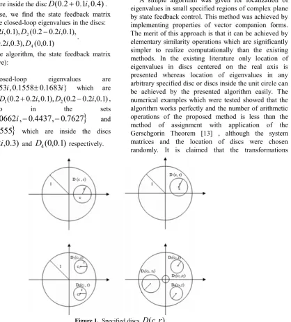
a disc

D

(

c

,

r

)

centered at

(

c

,

0

)

with radius r, in which

1





r

c

, as shown in Fig. 1. In this paper, the aim is to present a method for localization of eigenvalues in small specified regions of complex plane by state feedback control for discrete-time linear control systems.

Materials and Methods

Problem Statement

The problem of localization of eigenvalues in a small specified region has been the subject of many investigators in the last decades [2,6].

Consider a controllable linear time-invariant system defined by the state equation

 

t Ax

 

t Bu

 

t

x   (1)

or its discrete-time version

 

t Ax

 

t Bu

 

t

x 1   (2)

where

x

 

t





n,

u

 

t





mand the matrices

A

and

B

are real constant matrices of dimensions

n



n

and

n



m

respectively, with

rank

(

B

)



m

. The aim of eigenvalue assignment in a specified region is to design a state feedback controller,

K

, producing a closed-loop system with a satisfactory response by shifting controllable poles from undesirable to desirable locations. Karbassi and Bell [7,8], have introduced an algorithm for obtaining an explicit parametric controller matrix

K

by performing similarity operations on the controllable pair



B

,

A



. In fact,

K

is chosen such that the closed-loop system eigenvalues

BK

A







(3)

lie in the self conjugate eigenvalue spectrum





1

,



2

,



,



_n







. Recently, Karbassi and

Tehrani [9] extended the previous results as to obtain an explicit formula involving nonlinear parameters in the control law. The stabilization problem consists in finding a feedback matrix

K





mn _{such that the} input

u

_k



K

x

_k

,

k



0

,

,1

2

,...

, yields a stable closed loop system

,...

2

,1

,

0

,

)

(

1













A

BK

x

k

x

k k k (4)

In case the spectrum (or set of eigenvalues) of the

closed-loop matrix, denoted by



(



)

, is contained in the open unit disk we say that



is (Schur) stable or convergent (in other words,



_i



1

for all

)

(







i



). The stabilization problem arises in control problems such as, the computation of an initial approximate solution in Newton’s method for solving discrete-time algebraic Riccati equations, simple synthesis methods to design controllers, and many more [3, 11, 12].

The stabilization problem can in principal be solved as a pole assignment problem. Pole assignment methods compute a feedback matrix such that the closed-loop matrix of system (3) has a prespecified spectrum. In this paper, we present an efficient approach for localization of eigenvalues in small specified regions for linear discrete-time systems. Our assignment procedure is composed of two stages. We first obtain a primary state feedback matrix

F

_p which assigns all the eigenvalues of closed-loop system to zero, then produce a state feedback matrix

K

which assigns all the closed-loop system eigenvalues in a small specified disc or discs.

Synthesis

Consider the state transformation

 

t

T

x

 

t

x



~

(5)

where

T

can be obtained by elementary similarity operations as described in [7]. In this way,

AT

T

A

~



1 _and

B

~



T

1

B

_{are in a compact}

canonical form known as vector companion form:

  

 

  

  

 

m nm m

n

I G A

0 ___ __________

~ 0

 



 

  

  

 mm n

B B

0 _______

~ 0 ₍₆₎

Here

G

₀is an

m



n

matrix and

B

₀is an

m



m

upper triangular matrix. Note that if the Kronecker invariants of the pair



B

,

A



are regular, then

A

~

and

B

~

are always in the above form [7]. In the case of irregular Kronecker invariants, some rows of

I

_n_m in

A

~

are displaced [8]. It may also be concluded that if the vector companion form of

A

~

obtained from similarity operations has the above structure, then the Kronecker invariants associated with the pair



B

,

A



are regular [7].

(3)

eigenvalues to zero, for the transformed pair

 

B

~

,

A

~

, is then chosen as

x

F

x

G

B

u





01 0

~



~

(7)

Which results in the primary state feedback matrix for the pair



B

,

A



defined as

1

~





F

T

F

p (8)

The transformed closed-loop matrix

F

B

A

~

0







assumes a compact Jordan form with zero eigenvalues

















  



m m n m

n

n m

I

0

___

__________

0

~

0



(9)

Theorem 1: Let

D

be a block diagonal matrix in the form















k

D











0

2 1

(10)

where each

D

_j ,

(

j



,1

2

,...,

k

)

is either of the form

















j j

j j j

D









(11)

( to designate the complex conjugate eigenvalues

j j

i







)

or in case of real eigenvalues

]

[

j

d

D



(12)

If such block diagonal matrix

D

with self conjugate eigenvalue spectrum is added to the transformed closed-loop matrix,



~

₀, then the eigenvalues of the resulting matrix is the eigenvalues in the spectrum.

Proof:The primary compact Jordan form in the case of regular Kronecker invariants is in the form

















  



m m n m

n

n m

I

0

___

__________

0

~

0



(13)

The sum of



~

₀ with

D

has the form:

D

H

~





~

₀



(14)





























  



k m

m n m

n

n m

D

I













0

___

__________

0

₁

(15)

















k r

l l

D

I

D

I

D























0

1 1

2 1

(16)

where

I

_s

,

s



,1

2

,...,

r

is the unit matrix of size 2 in case

n



m

is even. In case

n



m

is odd only one

s

I

takes the form of a unit matrix of size one.

By expanding

det(

H

~





I

)

along the first row it is obvious that the eigenvalues of

H

~

are the same as the eigenvalues of

D

. For the case of irregular Kronecker invariants [8] only

some of the unit columns of

I

_n__m are displaced, since the unit elements are always below the main diagonal, the proof applies in the same manner.

Results

(4)

)

(

)

(

j

Column

i

Column





_j (17)

followed by

)

(

)

(

i

Row

j

Row





_j (18)

for j= n, n-1, …, m , i=j-m.

Hence, the matrix

H

~

_thus obtained will be in primary vector companion form such that:















  m n mm n

I

H

0

___

__________

~

0



 (19)

where

H

₀ is an

m



n

matrix .

Because of similarity operation, the eigenvalues of the matrix

H

~

 are the same as the eigenvalues of

H

~

and that of

D

. Now the feedback matrix of the pair

)

~

,

~

(

A

B

is defined by:

)

(

~

0 0 1 0 0 1

0

H

B

G

H

B

F

K













(20)

Theorem 2: The state feedback matrix

K

~

assigns the eigenvalues of closed-loop matrix

~





A

~



B

~

K

~

inside a circle with center

c

and radius

r

if in case circle intersects axis of abscissas we suppose



_j

,



_j be in the form:

)

Re(

)

1,

0

(

*

)

Im(

(

r

2

c

2

random

c

sqrt

j









(21)

)

1,

0

(

*

)

Im(

)

(

sqrt

r

2

l

2

c

random

j







₍₂₂₎

and in case circle does not intersect axis of abscissas we suppose

)

Re(

)

1,

0

(

*

random

c

r

j







(23)

)

Im(

)

1,

0

(

)

(

r

2

l

2

random

c

sqrt

j











(24)

where we take l



_j  Re(c) if



_j

*

Re(

c

)



0

and otherwise we take

l





j



Re(

c

)

and for assigning real valued eigenvalues in the

circle

c

and radius

r

we choose

)

Re(

)

1,

0

(

*

)

Im(

(

r

2

c

2

random

c

sqrt

d

j







(25)

Proof:The eigenvalues of matrix

D

defined above fall inside a circle with center

c

and radius

r

.

Let (26)



( )



0 0

~ ~ ~ ~

0 0 1 0 , 0

,

0 B _B _G _H

I G K

B A

m m n m m n m

n

            

    

 

 



(27)

   

       

 

  

 

 

m m n m

n m m n m

n I

H I

H B B G B B G

, 0

, 0 1 0 0 0 1 0 0 0

0 0

~

Clearly



~



H

~

, since

H

~

is similar to the matrix

H

~

and the eigenvalues of matrix

H

~

are the same as that of matrix

D

and elementary similarity operations do not change the eigenvalues, then the eigenvalues of closed-loop matrix



~



A

~



B

~

K

~

fall inside a circle with center

c

and radius

r

.

Remark: Since

K

~

assigns the eigenvalues of the closed-loop matrix



~



A

~



B

~

K

~

c

and radius

r

, it is obvious that the state

feedback controller matrix,

1 0 0 1 0

1

(

)

~













K

T

B

G

H

T

K

also assigns the

eigenvalues of the closed-loop matrix





A



BK

c

and radius

r

too.

Note that for assigning the eigenvalues of the closed-loop matrix in spectrum









₁

,



₂

,



,



_n



we suppose

n

j

D

_j





_j



,1

2

,



,

(28)

An algorithm for assignment of eigenvalues in a disc

)

,

(

c

r

D

.

In this section we first give an algorithm for finding a state feedback matrix which assigns zero eigenvalues to the closed-loop system. Then we determine a gain matrix which assigns the closed-loop eigenvalues in a circle with center

c

and radius

r

.

Input: The controllable pair

(

A

,

B

)

, the primary state feedback

F

_p,

B

₀1and

T

1which are calculated by the algorithm proposed by Karbassi and Bell [7,8], the center

c

and radius

r

of the target circle.

(5)

the form (10), in which for assigning complex valued eigenvalues in the circle with center

c

and radius

r

if circle intersects axis of abscissas we suppose

)

Re(

)

1,

0

(

*

)

Im(

(

r

2

c

2

random

c

sqrt

j









)

1,

0

(

*

)

Im(

)

(

sqrt

r

2

l

2

c

random

j







otherwise we choose

)

Re(

)

1,

0

(

*

random

c

r

j







)

Im(

)

1,

0

(

)

Re(

(

r

2

c

2

random

c

sqrt

j















where we take lj Re(c) if



j

*

Re(

c

)



0

and otherwise we take

l





j



Re(

c

)

and for assigning real valued eigenvalues in the circle

c

and radius

r

we choose

)

Re(

)

1,

0

(

*

)

Im(

(

r

2

c

2

random

c

sqrt

d

_j







Step 2. Set

H

~





~

₀



D

Step 3. Transform

H

~

to primary vector companion form

H

~

_as in (19) using elementary similarity operations as specified in corollary of theorem 1 .

step 4. Now compute 1 0 1 0 





F

B

H

T

K

p the

required state feedback matrix.

Illustrative Examples

Consider a discrete-time system given by



t



Ax

 

t Bu

 

t x 1  

Where

A

and

B

are randomly generated with

10



n

and

m



6

.















5

4

3

4

9

6

5

2

5

3

7

6

0

1

8

4

6

8

6

2

4

8

4

9

7

3

4

8

3

6

4

3

2

1

9

6

9

3

9

7

8

7

6

4

7

4

9

4

0

7

1

3

8

4

9

8

5

2

4

0

9

8

4

3

5

3

8

1

7

9

7

6

7

5

4

1

5

A















9

3

6

1

0

5

4

6

9

6

2

6

4

7

3

1

7

3

2

7

0

5

8

3

2

9

5

8

9

3

9

5

8

2

5

3

9

5

3

6

2

7

5

9

4

7

2

3

0

8

3

9

6

B

The open loop eigenvalues are

} 5948 . 47 , 2993 . 1 , 9397 . 9 , 2995 . 5 , 3189 . 7 5762 . 0 , 2589 . 4 8866 . 2 , 7729 . 3 3425 . 4 {     

 i i i

which are widely spread in the complex plane. In order to locate them in small discs inside the unit circle, we employ the above algorithm step by step. First, the primary state feedback matrix which locates all the eigenvalues of the closed-loop system to the origin of the complex plane is found to be:

(6)

Now we consider the following different cases: a) It is desired to locate the closed-loop eigenvalues inside the unit circle centered at origin. By using the algorithm, the state feedback matrix obtained is (above): It can be verified that the closed-loop eigenvalues are

,

}

6721

.

0

,

5252

.

0

,

2026

.

0

,

,

5

.

0

(

D

. By using the algorithm, the state feedback matrix obtained is (above):

The closed-loop eigenvalues are

,

}

3398

.

0

,

.

3

)

.

c) In this case, we find the state feedback matrix which assigns the closed-loop eigenvalues in the disc

.

02

)

. Clearly, localization of eigenvalues in small specified regions of complex plane by state feedback control is achieved.

d) In this case, we find the state feedback matrix which assigns the closed-loop eigenvalues in the disc

)

4

.

0

,

1

.

0

2

.

0

(

i

D



. By using the algorithm, the state feedback matrix obtained is (above):

(7)

The closed-loop eigenvalues are in the set

}, 1615 . 0 , 3704 . 0 , 2691 . 0 0761 . 0 , 0759 . 0

4814 . 0 , 0475 . 0 0884 . 0 , 1875 . 0 2829 . 0 {

 

 

 

i i

D

(

0

.

2



0

.

1

i

,

0

.

4

)

. e) In this case, we find the state feedback matrix which assigns the closed-loop eigenvalues in the discs:

)

1

.

2

.

0

(

4 3

2 1

D

i

D

i

D

i

D





.

By using the algorithm, the state feedback matrix obtained is (above):

The closed-loop eigenvalues are

}

1683

.

0

.

2



0

.

2

i

,

0

.

1

),

D

2

(

0

.

2



0

.

2

i

,

0

.

1

)

,

and also in the sets





0

0

,

2

.

0

6

.

0

(

3

i

D



and

D

₄

(

0

,

0

.

1

)

respectively.

Discussion

A simple algorithm was given for localization of eigenvalues in small specified regions of complex plane by state feedback control. This method was achieved by implementing properties of vector companion forms. The merit of this approach is that it can be achieved by elementary similarity operations which are significantly simpler to realize computationally than the existing methods. In the existing literature only location of eigenvalues in discs centered on the real axis is presented whereas location of eigenvalues in any arbitrary specified disc or discs inside the unit circle can be achieved by the presented algorithm easily. The numerical examples which were tested showed that the algorithm works perfectly and the number of arithmetic operations of the proposed method is less than the method of assignment with application of the Gerschgorin Theorem [13] , although the system matrices and the location of discs were chosen randomly. It is claimed that the transformations e)

       

 

       

 

 



 



2278 . 1 3592 . 0 6350 . 0 4175 . 0 0419 . 0 4418 . 0 6608 . 0 2148 . 0 2247 . 0 8390 . 0

4281 . 0 3386 . 0 8128 . 0 5913 . 0 4248 . 0 5576 . 0 1535 . 0 5908 . 0 4235 . 0 2601 . 0

2198 . 0 9973 . 0 8110 . 2 8173 . 0 2272 . 2 3166 . 0 2666 . 0 9463 . 0 3724 . 2 9936 . 1

7536 . 0 3282 . 0 4976 . 2 9830 . 1 1608 . 1 7287 . 0 0851 . 0 2602 . 0 0106 . 0 9824 . 0

5421 . 1 5491 . 0 3701 . 2 1543 . 0 5546 . 2 3688 . 0 3533 . 0 8530 . 0 9036 . 2 8658 . 1

4089 . 1 4604 . 0 8894 . 0 5998 . 0 9334 . 0 1762 . 0 3404 . 0 8331 . 0 0043 . 1 4979 . 0

K

(8)

obtained by similarity operations reduce accuracy of the computations [2], however, other methods such as LQR methods [10,11,15] and the method presented in [1,13] are more complicated.

References

1. Ayatollahi M. Maximal and minimal eigenvalue assignment for discrete-time periodic systems by state feedback.Optim. Lett,7: 1119-1123 (2013).

2. Benner P., Castillo M., and Quintana-orti E.S. Partial stabilization of large-scale discrete-time linear control systems. in: Technical Report, University of Bremen, Germany (2001).

3. Dragan V., and Halanay A. Stabilization of linear systems. in: Basel, Switzerland (1994).

4. Franke M. Eigenvalue assignment by static output feedback – on a new solvability condition and the computation of low gain feedback matrices.Int. J. Control,87: 64-75 (2014). 5. Fujinaka T., and Katayama T. Discrete-time optimal

regulator with closed-loop poles in a prescribed region.Int. J. Control,47:1307-1321 (1988).

6. Grammont L., and Largillier A. Krylov method revisited with an application to the localization of eigenvalues.

Numer. Func. Anal. Opt,27: 583-618 (2006).

7. Karbassi S.M., and Bell D.J. Parametric time-optimal

control of linear discrete-time systems by state feedback-Part 1: Regular Kronecker invariants. Int. J. Control, 57: 817-830 (1993).

8. Karbassi S.M., and Bell D.J. Parametric time-optimal control of linear discrete-time systems by state feedback-Part 2: Irregular Kronecker invariants. Int. J. Control,57: 831-839 (1993).

9. Karbassi S.M., and Tehrani H.A. Parameterizations of the state feedback controllers for linear multivariable systems.

Comput. Math. Appl,44:1057-1065 (2002).

10. Kawasaki N., and shimemura E. Determining quadratic weighting matrices to locate poles in a specified region.

Automatica,19:557-560 (1983).

11. Mehrmann V. The autonomous linear quadratic control problem. theory and numerical solution, In: Lecture notes in control and information sciences, Springer-verlag, Heidelberg (1991).

12. Sima V. Algorithms for linear quadratic optimization Pure and applied mathematics, New York (1996).

13. Tehrani H.A. Assignment of Eigenvalues in a Disc D(c,r) of Complex Plane with Application of the Gerschgorin Theorem.World Appl. Sci. J,5(5): 576–581 (2008). 14. Yuan L., Achenie L.E.K., and Jiang W. Linear quadratic

optimal output feedback control for systems with poles in a specified region.Int. J. Control,64: 1151-1164 (1996). 15. Zhou B., Cai G., and Duan G. Stabilisation of time-varying