Robust sensorless vector control of induction machines

Printed in The Islamic Republic of Iran, 2009 © Shiraz University

ROBUST SENSORLESS VECTOR CONTROL OF INDUCTION MACHINES*

R. KIANINEZHAD1,** B. NAHID-MOBARAKEH2, F. BETIN3 AND G.A. CAPOLINO3

1

Shahid Chamran University, Ahvaz, 61355, I. R. of Iran Email: [email protected]

2

Institut National Polytechnique de Lorraine, Nancy, France,

3

University of Picardie Jules-Verne, 13 Av François Mitterrand, 02880, Cuffies, France

Abstract– A sensorless vector control strategy for induction machine (IM) operating in variable speed systems is presented. The sensorless control is based on a reduced-order linear observer based on terminal voltage and current as input signals. An estimation algorithm based on this observer is proposed to compute speed. It is shown that the proposed sensorless control is more sensitive to the stator resistance than to the rotor resistance. In order to tune the observer and to compensate for the parameter variations and the uncertainties, a separate estimation of the stator resistance is introduced. The equations to estimate the stator resistance are derived from the machine differential equations. For certain operating regions of the machine, it is verified that the stator resistance can be accurately estimated regardless of wide stator resistance variation. It is shown that design and hardware implementation of this method is simpler than the previous works. The simulation and experimental results demonstrate the good performance of the proposed observer and estimation algorithm and of the overall indirect-field-oriented-controlled system.

Keywords– Sensorless control, induction machine, observer, parameter identification

1. INTRODUCTION

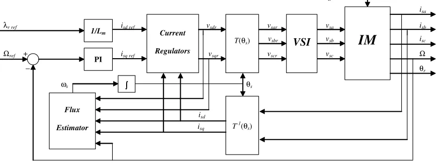
Induction machines (IM) are widely used in industry. They have a simple and robust rotor design and offer high efficiency, low cost and maintenance. In torque control, the dynamic requirements are often satisfied by using field oriented control (FOC). The FOC strategy has become a standard in the control of IM and consists in controlling the stator current vector in a 0dq reference frame using a proper rotation [1-2]. This rotation, defined by a vector control law, improves the IM control by decoupling the flux control and the torque control: the d-component of the stator current is used to control the flux, while the torque is controlled by the q-component of the stator current (Fig. 1). Thus, the control performances depend on this decoupling condition which is based on the vector control law [1].

The main drawback of the FOC is that the shaft speed (or position) feedback is required. This presents a huge problem for low cost systems in which motor mechanical sensors are not available. This has led to sensorless control of AC machines, a field of research during the past decade [3-13]. Sensorless control of induction motors has faced two kinds of methods: the one which uses the dynamic model of the induction machine based on the fundamental spatial harmonic of the magnetomotive force (mmf) [4–11], and the other based on the saliencies of the machine [12] [13] which are based on high-frequency signal injection. Among the first, the main one is the open-loop speed estimators [4], MRAS (model reference adaptive system) speed observers [5] [6], full-order observers [7] [8], and reduced order speed observers [9-11]. Most of these methods are applied with vector control by rotor field orientation and are based on the different complex models which require large computation time. The full-order observer gives very

∗

Received by the editors June 23, 2008; Accepted April 16, 2009. ∗∗

interesting performances with a significant computational requirement, one of the main problem of speed observers.

ΤL

isa

λr ref isd ref vsdr vsar vsa isb

vsbr vsb isc

Ωref + isq ref vsqr vscr vsc Ω

− θr

ωs θs

isd

isq Current

Regulators VSI

IM

T-1(θs)

T(θs) 1/Lm

PI

Flux

Estimator

Fig. 1. Block scheme for vector control of an induction machine

The goal of this work is the design of a simple speed observer with a performance closed to the one obtainable with a full-order observer. This is achieved by a reduced- order rotor flux observer, giving in lower complexity and computational burden. In fact, the Reduced-order observer has to solve a problem of order less than four while the full-order observer solves a problem of order four. Different from [5], which employs a combination of the reduced-order observer used as the reference model, and the simple current model used as the adaptive model to estimate the rotor speed, here the reduced-order observer is only used for rotor speed estimation just on the basis of the stator current measurements and the estimated flux. In particular, this paper presents a new sensorless technique based on the reduced-order observer with an on-line estimation of the stator resistance. The main advantage of this observer is that it is very simple to design and it reduces computational cost time. The proposed sensorless vector-controlled system is designed to fulfil the following requirements:

- decoupled stator flux and electromagnetic torque control - stator-current limitation under all operating conditions

- accurate flux estimation based only on stator current measurement - accurate speed estimation without the use of additional measurement - stable speed control over a wide operating area

- simplification of the required algorithms to obtain a low computation time - minimization of the required current and voltage sensors

For a detailed study of the controlled drive system, a model of the overall system has been developed using the MATLAB/SIMULINK software. Indeed, it has been implemented experimentally on a conventional DSP (TMS320C31) associated with a coprocessor (ADMC201) dedicated to the control of IM and compared with the classic full-order adaptive observer.

respect to the parameter uncertainties. It is shown that the proposed observer is widely sensitive to variations of the stator resistance. To overcome this problem, an on-line stator resistance identification method is added in the sixth part. The experimental results of the proposed method have been shown in the seventh part. Finally, some conclusions and perspectives will be discussed.

2. SYSTEM PRESENTATION

a) Experimental test bed

To test the capacities of the proposed sensorless control algorithm, an advanced test-bed has been built around:

- a 750 W three-phase squirrel-cage induction machine with a shaft-mounted optical encoder (1024 points per revolution)

- a three-phase rectifier

- an insulated gate bipolar transistor (IGBT) voltage source inverter (VSI) - three Hall-effect current sensors for measurement of stator currents - variable inertia disks and an electromechanical powder brake

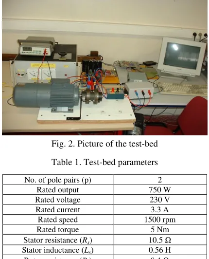
The experimental system configuration is shown in Fig. 2 and its parameters are given in Table 1. The machine is controlled by a DSP (TMS320C31) associated to a coprocessor (ADMC201) dedicated to the control of IM. The sampling frequency is fixed at 5 kHz and the controller receives the stator currents measurements through two 8- bit A/D converters. Then, using the PWM technique, the reference voltages are sent to the machine via the voltage-source inverter whose switching frequency is fixed at 5 kHz. Based on this system and the following model, a program to simulate the dynamics of the IM and its load has been developed.

Fig. 2. Picture of the test-bed

Table 1. Test-bed parameters

No. of pole pairs (p) 2

Rated output 750 W

Rated voltage 230 V

Rated current 3.3 A

Rated speed 1500 rpm

Rated torque 5 Nm

Stator resistance (Rs) 10.5 Ω

Stator inductance (L_s) 0.56 H Rotor resistance (Rr) 8.4 Ω

Rotor inductance (Lr) 0.56 H

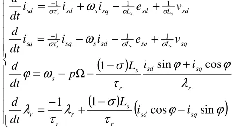
b) IM model

Let us consider a 0dq reference frame (Fig. 3) in which the electrical unsaturated model of the induction machine can be described as follows [14]:

(

)

(

−

Ω

)

−

+

=

Ω

−

+

+

=

+

Ω

−

+

−

=

+

Ω

+

+

+

=

p

i

dt

d

p

i

dt

d

v

p

i

i

i

dt

d

v

p

i

i

i

dt

d

λ

ω

λ

λ

λ

ω

λ

λ

λ

λ

ω

λ

λ

ω

q ωs

d

λr ωr=pΩ

ϕ αr

θs θr

αs

Fig. 3. 0dq and 0αβ reference frames

The machine parameters are Rs, Rr, Lr, Lm, Ls and p (Table 1), with:

r s 2 m L L L 1− = σ r s m L L L = µ eq s s R L s= ′ τ , r r R L r=

τ _r

L L s eq

s R R

R ₂ r 2 m + =

The mechanical equation is:

( )

Ω Tm TL

dt d

J = − (2)

where J is the inertia coefficient, and:

(

)

pL

m i i

T

r

m _{λ −λ}

= (3)

is the torque generated by the motor and TL is the load torque supposed to be unknown.

where the following change of coordinates is used: ϕ λ λ ϕ λ λ sin cos r L L rq r L L rd m r m r − = = (5)

In the model (4), esd and esq denote d-q components of the back-EMF vector.

The second terms in (6) may not be considered as the back-EMF. But esd and esq are the back-EMF vector

components taken for simplicity purpose.

+ Ω = − Ω = ϕ λ ϕ λ ϕ λ ϕ λ τ τ sin cos cos sin 1 1 r r sq r r sd r r p e p e (6)

The mechanical equation is :

(

)

( )

λ = Ω _L J sq sd r J p T cos i sin i dt

d _{1 (7)}

3. VECTOR CONTROL OF IM

According to model (4), if ϕ is going to zero (or 2kπ), the rotor flux becomes independent from isq while

the machine torque is proportional to isq. This is the objective of the vector control. The only degree of

freedom is the angular speed of 0dq reference frame ωs which must be used to set ϕ to zero. According to

(4), the stator voltage angular frequency ωs is determined by the following vector control law [10]:

(

)

ω 1 (8)

It can be easily shown that this vector control law guarantees the setting of ϕ to zero if the motor parameters are well-known [10]. Replacing (8) in (4) and simplifying (6) and (7), the following equations, which describe the dynamic behavior of the vector-controlled IM, can be written as:

( ) + λ = λ + λ + ω + = τ σ − τ − σ τ σ τ′ σ − sd L r r sd L r L sq s sd sd i dt d v i i i dt d r s r s r s s 1 1 1 1 1 (9a) − λ = Ω + Ω λ − ω −

=_σ−_{τ′ σ σ}

L J sq r J p sq L r L p sd s sq sq T i dt d v i i i dt d s s s 1 1 1 (9b)

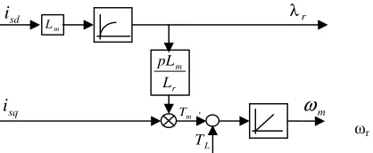
As it can be seen from (9a), the rotor flux does not depend on the load torque nor on isq, if ϕ is well

set to zero. Equation (9b) shows that the angular speed Ω depends on the load torque and on the electromagnetic torque which depends on the rotor flux and on isq (Fig. 4). Thus, the model (1)-(3) is

decomposed in two subsystems (9a) and (9b). It leads to use only the second subsystem in order to estimate the angular speed.

Fig. 4. Block scheme of decoupling control

4. MECHANICAL SENSORLESS CONTROL METHOD

In the mechanical sensorless control, the angular speed (or position) measurement is substituted by its estimation. A large number of estimation methods have been proposed since the early nineties. In this paper a linear reduced order disturbance observer in order to estimate the rotor angular speed is proposed. In the previous section, the decomposed model (9) has been presented. As it can be seen in (9b), the angular speed estimation requires knowledge of the load torque and the rotor flux. Supposing that the load changes slowly, it can be written:

0

≅

L

T dt

d ₍₁₀₎

This assumption is correct in most applications. Adding (10) to (9b), it can be shown:

= − = Ω + Ω − − = −_′ 0 1 1 1 L L J sq r J p sq L r L p sd s sq sq T dt d T i dt d v i i i dt d s s s

λ

λ

ω

τ σ

(11)

From (11), and supposing that λr is constant by holding isd constant, one may propose the following linear

disturbance observer:

=

+

−

=

Ω

+

+

Ω

−

−

=

i

K

T

dt

d

i

K

T

i

dt

d

i

K

v

i

i

i

dt

d

~

ˆ

~

ˆ

ˆ

ˆ

~

ˆ

ˆ

ˆ

λ

λ

ω

τ σ

(12)

with i~_sq=iˆ_sq−i_sq, and:

( ) sd L r r

i

dt

d

λ

λ

=

+

(13)

The observer gains K1 to K3 are obtained by applying a linear pole placement technique to the estimation error equations described as follows:

= − + = Ω Ω − + − = sq L L sq r r L p sq s sq i K T dt d T J i K J p dt d i K i dt d s ~ ~ ~ 1 ~ ~ ~ ~ 1 ~ 3 2 1 '

λ

λ

στ

139

It has to be noted that in the observer (12), λr is considered to be constant. It is not true during the first time of the transient while the motor is not properly magnetized. But within this period, the machine torque (controlled by isq), as well as its angular speed, is generally controlled to zero. This prevents the

divergence of the estimated variables. Then, the observer works as a linear one when the machine is magnetized.

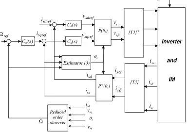
The observer (12) does not require high computational cost and is easy to implement on a classical processor. In order to validate the performance of the proposed method, a simulation program using Simulink-Matlab software based on the proposed algorithm and on setup parameters have been developped. Fig. 5 shows the simulation scheme.

Equations (8) and (13) have been respectively used to estimate the orientation of the rotor flux and its amplitude. PI regulators are also used to control the current and the speed. The angular speed is estimated by the reduced-order observer (12) and it should be noted that the stator current components (isa and isb)

are the only variables used in the sensorless control algorithm.

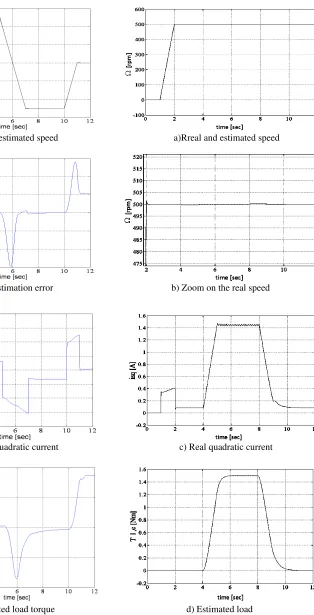
Figure 6a depicts the real speed and the estimated speed using the simulation program and Fig. 6b represents speed estimation error. Fig. 6c and 6d depict, respectively, the quadratic current and the estimated load torque for a startup, a steady state at 500 rpm and a speed inversion test. It can be noted from this simulation test that the estimated speed is very close to the real speed. Also the estimated load torque is practically equal to TL=0,except during the speed inversion. In order to study the disturbance

rejection using the proposed method, a new test has been performed when a load torque step (Tl=1.5 N.m)

occurs at time t=4s up to time t=8s. Figure 7a represents the real and the estimated speed, Fig. 7b depicts a zoom of the real speed, Fig. 7c represents the real quadratic current and Fig. 7.d depicts the estimated load. From this test, it can be noted that the real speed and the estimated speed are close and they follow the reference speed while the load torque is correctly estimated.

Fig. 5. Block scheme used for simulation

ch

sdref

i

ref Ω

sdref

v

sqref

v

Cd(s)

Cq(s) C (s)

P( s)

α

s

v

β

s

v

sa

i

sb

i

sc

i

α s

i

β s

i

sq

i

[T3]-1

s

[T3] P-1( s)

Inverter

and

IM

Ω

sd

i

sqref

i

Reduced order observer

isd

isq

s

vsq

a) Real and estimated speed a)Rreal and estimated speed

b) Speed estimation error b) Zoom on the real speed

c) Real quadratic current c) Real quadratic current

d) Estimated load torque d) Estimated load

Fig. 6. Simulation results for a startup and a speed Fig. 7. Simulation results for a load torque rejection test

141

5. ROBUSTNESS STUDY

This sensorless control method is suitable for medium and high speed applications, if there is no important parameter uncertainty. Indeed, the electrical parameters of the IM are supposed to be known and do not change. Nevertheless, it is not true in practice because of model or parameter uncertainties and measurement noises. Therefore, the sensitivity of the proposed method with respect to the electrical motor parameters uncertainties, particularly to the stator and rotor resistance variations has been tested. Figures 8a and 8b depict, respectively, the estimated motor speed and the difference between the reference and the motor speed error for +50% error in the rotor resistance. Figs. 8c and 8d depict, respectively, the motor speed and the difference between the reference and the motor speed error for +50% error in the stator resistance. It can be noticed that the proposed sensorless control estimation is more sensitive to the stator resistance than to the rotor resistance. In the next section, a new on-line identification method will be introduced in order to obtain an estimation of the stator resistance during the motion.

a) Motor speed for +50% error in Rr b) Motor speed error for +50% error in Rr

c) Motor speed for +50% error in Rs d) Motor speed error for +50% error in Rs

Fig. 8. Responses with rotor or stator uncertainties

6. ON-LINE IDENTIFICATION OF STATOR RESISTANCE

sd L rd r L sq s sd L R

sd i i R v

i dt d s r s seq σ σ µ

σ

ω

λ

1

+ +

+

= − (15)

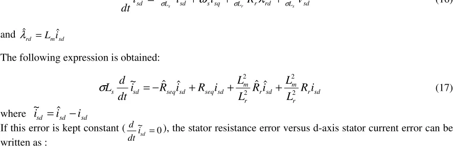
From the previous equation, the d-axis stator current error due to the both stator and rotor resistance errors can be obtained. Indeed, by considering:

sd L rd r L sq s sd L R

sd i i R v

i dt d s r s seq σ σ µ

σ

ω

λ

ˆ

ˆ ˆ ˆ

ˆ ₌ − _{+ + +}

(16)

and λˆ_rd =L_miˆ_sd

The following expression is obtained:

sd r r m sd r r m sd seq sd seq sd

s Ri

L L i R L L i R i R i dt d L ₂ 2 2 2 ˆ ˆ ˆ ˆ ~ + + + − =

σ

where

~

i

=

i

ˆ

−

i

If this error is kept constant ( ~i_sd =₀

dt

d _{), the stator resistance error versus d-axis stator current error can be}

written as :

sd sd s s i i R R ~ ˆ ~ = (18)

The Appendix 1 gives the required computation for obtaining this formula.

Based on the last results, the following stator resistance estimator has been introduced:

dt i R t R t sd

s = −

0 0

~ )

(

ˆ

α

To compute the d-component stator current error, the following estimator is used:

sd L sq s sd L R

sd i i v

i dt d s s s σ σ ω 1 ˆ ˆ

ˆ ₌ − _{+ + (20)}

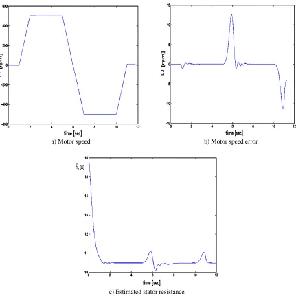
Figure 9a and Fig. 9b represent the motor angular speed and the motor angular speed error with the stator resistance estimator, respectively. The initial error is fixed at 15.75 Ω which corresponds to 50% as on Fig. 8c and 8d. By comparing Figs. 9b and 8d, it can be seen that the speed error is reduced using the stator resistance estimator. Figure 9c depicts the evolution of the estimated stator resistance. It can be seen that after 1 sec., the estimated stator resistance has reached the real value (almost 10.5Ω)

7. EXPERIMENTAL VALIDATION

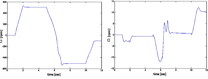
Figure 10a depicts the experimental motor speed and the estimated speed, while Figs. 10b and 10c show the speed estimation error and the real quadratic current for a trapezoidal speed profile with a steady state at 500 rpm and a speed inversion. It can be noticed that the speed estimation error during the steady state is reduced since its maximum value is about +/- 8 rpm.

143

From this experimental test, it can be seen that the estimation error is still reduced and that the tracking capacities are good.

a) Motor speed b) Motor speed error

c) Estimated stator resistance

Fig. 9. Response with RS estimation and 50% initial error

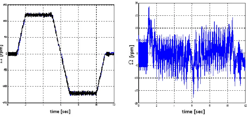
Figure 12a shows the experimental motor speed and the estimated speed, while Fig. 11b depicts the speed estimation error for a speed trapezoidal profile with a steady state at 60 rpm and a speed inversion. It can be seen that the estimated speed trajectory follows the real speed trajectory and the angular speed follows its reference. However the relative estimation error is higher than the previous cases.

a) Real and estimated speed b) Speed estimation error

c) Real quadratic current

Fig. 10. Experimental results at high speed

145

a) Real and estimated speed b) Speed estimation error

Fig. 12. Experimental results at low speed (60 rpm)

8. CONCLUSION

In this paper a new reduced-order observer for sensorless control of induction machines associated with an on-line estimation of the stator resistance has been proposed. The proposed method uses a reduced-order observer of order three that simplifies computation of speed estimation. It has been shown that this method is more sensitive to the stator resistance variations than to the rotor resistance variations. Therefore a new estimator of stator resistance has been introduced to overcome this problem.

The proposed approach has been implemented successfully on a low cost DSP (TMS320C31) associated with a dedicated coprocessor (ADMC201). The experimental results have shown the performance of the proposed method down to 60 rpm. Furthermore, the tracking capacities have been validated experimentally using speed trapezoidal profiles with speed inversion.

Besides the fact that this approach presents good tracking and regulation capacities, the main advantage of this observer is that the estimation time is reduced. Indeed, it takes only 8 µs on the TMS320C31, while the classical method requires about 30 µs. Furthermore, it has been proved that by adding a stator resistance estimator, the proposed approach is completely insensitive to uncertainties on the stator resistance.

Acknowledgment- This work has been supported by the Center for International Research and Collaboration (ISMO) and the French Embassy in Tehran. The experimental results were obtained in the Laboratory of Innovative Technologies of the University Picardie < Jules Verne > in France.

NOMENCLATURE

Rs stator resistance vs stator voltage

Rr rotor resistance ir rotor current

Ls stator inductance vr rotor voltage

Lr rotor inductance e back-emf

τr rotor time constant p number of pole pairs

τs stator time constant J inertia coefficient

Lm mutual inductance Ω rotor angular speed

is stator current s angular speed 0dq frame

θs position of 0dqframe r rotor

θ rotor position 0 α β stationary coordinates

ϑ position of 0δγ frame 0 d q synchronous coordinates

ϕ rotor position error (ϕ = ϑ – θ) 0 δ γ control coordinates

Τm electromagnetic torque Superscripts

ΤL load torque ^ estimated value

Subscripts ~ error value

a, b ,c phases

s stator

REFERENCES

1. Leonhard, W. (1996). Control of electrical drives. Springer-Verlag.

2. Marino, R., Peresada, S. & Valigi, S. (1993). Adaptive input–output linearizing control of induction motors.

IEEE Trans. AC, Vol. 38, No. 2, pp. 208–211.

3. Vas, P. (1998). Sensorless vector and direct torque control. Oxford University Press.

4. Holtz, J. & Juntao, Q. (2003). Drift- and parameter-compensated flux estimator for persistent

zero-stator-frequency operation of sensorless-controlled induction motors. IEEE Trans. Ind. Appl., Vol. 39, pp. 1052–1060.

5. Tajima, H. & Hori, Y. (1993). Speed sensor-less field-orientation control of the induction machine. IEEE Trans.

Ind. Applicat., Vol. 29, pp. 175-180.

6. Soltani, J., Abdolmaleki, Y. & Hajian, M. (2005). Adaptive fuzzy sliding-mode control of speed sensorless

universal field oriented induction motor drive with on-line stator resistance tuning. Iranian Journal of Science &

Technology, Transaction B, Engineering, Vol. 29, No. B4.

7. Kim, Y. R., Sul, S. K. & Park, M. H. (1994). Speed sensorless vector control of induction motor using extended

Kalman filter. IEEE Trans. Ind. Applicat., Vol. 30, No. 5, pp. 1225–1233.

8. Kubota, H., Sato, I., Tamura, Y., Matsuse, K., Ohta, H. & Hori, Y. (2001). Stable operation of adaptive observer

based sensorless induction motor drives in regenerating mode at low speeds. in Proc. IAS Annu. Meeting, pp.

469–474.

9. Song, J., Lee, K. B., Song, J. H., Choy, I. & Kim, K. B. (2000). Sensorless vector control of induction motor

using a novel Reduced-order extended Luenberger observer. in Proc. Record IEEE Conf. Industry Appl., Vol. 3,

pp. 1828–1834.

10. Kianinezhad, R., Nahidmobarakeh, B., Betin, F. & Capolino, G. A. (2004). Observer-based sensorless

field-oriented control of induction machines. IEEE International Symposium on Industriall Electronics, ISIE, France.

11. Cirrincione, M.,Pucci, M., Cirrincione, G. & Capolino, G. A.(2007). Sensorless control of induction motors by

reduced-order observer with MCA EXIN + based adaptive speed estimation. IEEE Trans. On Industrial

Electronics, Vol. 54, No. 1, pp. 150-166.

12. Caruana, C., Asher, G. M. & Sumner, M. (2006). Performance of HF signal injection techniques for

zero-low-frequency vector control of induction machines under sensorless conditions. IEEE Trans. On Industrial

Electronics, Vol. 53, No. 1, pp. 225-238.

13. Wang, G., Hofmann, H. F. & El-Antably, A. (2006). Speed-sensorless torque control of induction machine based

on carrier signal injection and smooth-air-gap induction machine model. IEEE Trans. On Energy Conversion,

Vol. 21, No. 3, pp. 699-707.

14. Grellet, G. & Clerc, G. (1995). Actionneurs électriques. Editions Eyrolles, Paris.

15. Nahidmobarakeh, B., Betin, F., Pinchon, D. & Capolino G. A. (2003). Sensorless field oriented control of

147

Appendix 1

Equations (16)-(17) yield:

(A1)

Replacing in (A1) yields:

(A2)

:

Using and

(A3)

(A4)

Replacing :

(A5)

(A6)

_(A7)

If this error is kept constant ( ~ ₌₀

sd

i dt

d _{), the stator resistance error versus d-axis stator current error can be explained}

as: (A8) sd r r m sd r r m sd seq sd seq sd

s Ri

L L i R L L i R i R i dt d L ₂ 2 2 2 ˆ ˆ ˆ ˆ ~ + + + − =

σ

r R R

Rˆ = + ~

sd r r m sd r r m sd seq sd seq sd

s R i

L L i R L L i R i R i dt d

L ~ ˆ ˆ ~ˆ ₂ ~

2 2 2 + + + − =

σ

seq R R

Rˆ = +~

i

ˆ

=

i

+

i

~

sd r r m sd r r m sd seq sd sd seq seq sd

s R i

L L i R L L i R i i R R i dt d

L ~ ( ~ )( ~ ) ~ ˆ ₂ ~

2 2 2 + + + + + − =

σ

s R i

L L i R i R L L i R i dt d

L ~ ~ ~ˆ ~ ₂ ~

2 2 2 + − + − =

σ

s R R

R r m 2 2 + = sd s sd r r m sd seq sd

s Ri R i

L L i R i dt d

L ~ ~ ₂ ~ˆ ~

2 − + − =

σ

s Ri R i

L L i i R L L R i dt d

L ~ ( ~ ~ )(ˆ ~ ) ₂ ~ˆ ~

2 2 2 − + − − − =

σ

s i Ri R i

dt d

L ~ =−~ˆ − ~