Iranian Journal of Economic Studies
Journal homepage: ijes.shirazu.ac.ir
Optimal Cyclical Behavior of Monetary Policy of Iran: Using a DSGE Model
Neda Kasaipour, Alireza Erfani
Department of Economics, Semnan University, Semnan, Iran.
Article History Abstract
Received date: 07 April 2018 Revised date: 02 May 2018 Accepted date: 07 May 2018 Available online: 20 May 2018
The countercyclical monetary policy is a policy that economists recommend to adopt in order to slow down the economic fluctuations. The aim of this study is to address the question that, in the presence of fiscal dominance and considering institutional quality (IQL), what the optimal monetary policy should be during the business cycles? To find the appropriate answer, first, in the framework of a Dynamic Stochastic General Equilibrium (DSGE) model, proportional to the structure of the Iranian economy, the parameters of the model are derived. Then, considering fiscal dominance and institutional quality, the optimal monetary policy during the business cycles is calculated and by using the equilibrium parameters, using data of Iran during 1991:2-2016:1, it is calibrated. The results show that the optimal monetary policy during business cycles of Iran is a countercyclical monetary policy. The optimal monetary policy coefficient during the business cycles decreases by a decline in institutional quality and an increase in fiscal dominance. In addition, when the policymaker's goal is only stabilizing inflation, the optimal monetary policy is independent of the business cycles. In addition, when the monetary policy is assumed completely independent, the optimal policy coefficient takes the highest value compared to the other assumed conditions.
JEL Classification: C11
C61 E02 E12
Keywords: Monetary Policy Business Cycles
Dynamic Stochastic General Equilibrium (DSGE)
1. Introduction
A procyclical monetary policy is implemented when the main monetary policy tool, is interest rate and if the interest rate is raised during recessions, but lowered during expansions, i.e. booms. A procyclical monetary policy is also implemented when the main monetary policy tool, is money supply and if money supply is decreased during recessions but increased during expansions. In other words, if a contractionary monetary policy is adopted during recessions and an expansionary monetary policy is adopted during expansions, the followed monetary policy is of procyclical type and leads to larger economic fluctuations (Duncan, 2014).
[email protected]
The findings of some studies, such as Frenkel et al. (2011) and Végh and Vuletin (2012) have demonstrated a sharp contrast between industrialized and developing countries in terms of cyclicality of economic policies. Since 1960, a large number of developing countries have followed a significant level of procyclical fiscal and monetary policies. Most developed countries, however, have supported a cyclical or countercyclical policy regime over the same period. The large number of studies have been conducted in an attempt to explain this controversial issue, and they have mainly focused on political economy by taking into account either economic theories or microeconomic financial assumptions (Kim, 2014). The reason for these countries' inability to follow optimal stabilization policies, i.e. countercyclical policies, can be due to such constraints as restrictions on borrowing from abroad, fragile domestic financial systems, enormous external debt, political economy constraints, lack of political credit, corruption, and incomplete information about government programs (Calderon et al., 2012).
It should be noted that weak political parties, political instability, political pressures, weak rule of law, and bureaucratic corruption are among major indicators of many developing countries with weak institutional quality. These characteristics make framing of optimal monetary and fiscal policies in these countries different from that in countries with good institutional quality. The absence of active parties and political organizations, the existence of pressure groups, and political instability will lead to an increase in government expenditures. However, due to weak rule of law and bureaucratic corruption, government extractive capacity is very small. Therefore, every government usually tries to pays special attention to seigniorage in order to finance its heavy expenditures and to adopt inflationary fiscal policies to make more money. In an economy with a weak institutional quality, however, due to the overwhelming fiscal dominance, the central bank cannot be independent and the monetary policy is passive. On the other hand, pursuing an inflation targeting policy becomes weaker due to fiscal dominance (Gruben and Welch, 2010). The absence of inflation targeting will also complicate the adoption of countercyclical monetary policies through destroying political credibility. Therefore, fiscal dominance causes monetary policy to be of a procyclical type.
This paper is organized as follow: The relevant literature will be reviewed. Next, a DSGE model will be proposed. The study, then, focuses on the way the optimal cyclical monetary policy is derived. After that, the data will be analyzed and model parameters will be calibrated. Finally, the study's conclusions will be drawn.
2. Literature Review
Many studies have been conducted on the empirical determination of cyclicality (cyclical behavior) of monetary policy during business cycles. Few studies, however, have focused on the optimal cyclical behavior of monetary policy. This section provides the readers with a summary of a few of the studies conducted in the field of optimal cyclical monetary policy.
To understand the reason for the difference in cyclicality behavior of monetary policies of the developing and developed countries, Yakhin (2008)
constructed a New-Keynesian open economy model. In this model, the optimal monetary policy has been achieved by taking into account different levels of the international financial market integration. Yakhin (2008) observed that the optimal monetary policy was a countercyclical policy. The results indicated that when economies gained access to international financial markets, their optimal monetary policy varied from procyclical to countercyclical.
Duncan (2014) investigated the relationship between institutional quality, cyclicality of monetary policy and output volatility. The researcher has used an extended standard DSGE model to determine the behavior of investors facing institutional risk. In this model, by adopting discretionary policies, the central bank seeks to stabilize inflation and output volatility. Foreign agents are directly investing in the economy and grant households foreign loans to finance their consumption and other expenditures. Foreign investors face the possibility of product losses due to changing of institutional quality. The model was calibrated using data from Indonesia. Result of the models showed a negative relationship between the production and the nominal interest rate that is associated with the low levels of institutional quality.
In another study on cyclicality of monetary policy, Kim (2014) examined cyclical behavior of monetary and fiscal policies through using a New Keynesian DSGE model. The study theoretically investigated the optimal monetary and fiscal policies in an economy where an imperfect infrastructural development influences the dynamics and behavior of consolidated policies. By solving a Ramsey policy problem the researcher concluded that in the presence of imperfect infrastructural development, the optimal fiscal and monetary policies tend to be more procyclical and the economy experiences more volatile. In addition, by comparing different monetary policy regimes, based on Taylor rule, Kim (2014) also claimed that inflation targeting rule reduces procyclical behavior of fiscal and monetary policies and improves welfare.
- Access to international financial (capital) markets - Institutional risk faced by foreign investors. - Imperfect infrastructural development
This study is distinct from other relevant studies, which considers institutional quality as well as fiscal dominance in the domestic economy. In fact, this study is based on Duncan (2014). The following modifications, however, have been made in this work:
- Duncan (2014) has used a small open economy model in which foreign investors face problems due to weak institutional quality. In the present study, however, weaknesses of institutional quality are considered in government budget constraint.
- Duncan (2014) has considered interest rate as central bank's tool. Given the free-interest banking system of Iran, however, central bank's tool is money supply.
In this study, government sector has been added to the model, and thus fiscal dominance in Iran's economy has been taken into consideration.
3. Theoretical Background
Optimal monetary policy, without considering fiscal dominance, is not a wise choice for economies with weak institutions. Hence, this section provides a partial explanation about cyclical monetary policy in the presence of fiscal dominance and institutional quality.
If a fiscal policymaker set his expenditures, regardless of the intertemporal budget balance, and if the present discounted value of taxes to finance expenditures, in terms of present value, is insufficient, the budget must be balanced through seigniorage. Such a regime is a fiscal dominant regime in which fiscal policy is active but monetary policy is passive because the monetary policy should be set so that the amount of seigniorage can balance the budget. In this kind of regime, prices and inflation will be affected by changes in fiscal policy. (Walsh, 2010)
The discussion of fiscal dominance was given special significance in economic texts after the Sargent and Wallace's (1981) seminal work entitled "unpleasant monetarist arithmetic" and then, work entitled "the fiscal theory of the price level" by Woodford (2003).
economy. Hyper crowding-out effect may cause contractionary fiscal policy to have an expansionary effect (Gruben and Welch, 2010). Therefore, procyclical fiscal policy should be adopted in these circumstances. During a recession, a contractionary fiscal policy must be adopted so that its expansionary effects can lead to an increase in output and the economy will exit from the recession. But, given the hyper crowding-out effect, this contractionary fiscal policy can dramatically reduce real interest rates by reducing government's expenditures. To reduce economic fluctuations, the adopted monetary policy of this economy must lead to an increase in interest rates. Thus, the adopted monetary policy must also be contractionary. Hence, in fiscally dominant economies, hyper crowding-out phenomenon may lead to adoption of a procyclical monetary policy.
Douglas North (1993), the co-recipient of the Nobel Prize in economics, strongly emphasizes the role of institutions in the economy. He states that institutions' effect on economic performance is not very controversial and everyone has more or less accepted it. The issue of institutional quality can be expressed in form of good governance. In economic literature, good governance includes indicators, such as voice and accountability, political stability and absence of violence, government effectiveness, regulatory quality, rule of law, and control of corruption. From among the indicators of institutional quality, the index that is more attractive to researchers in the field of monetary policy is the corruption index. It seems the best way for adding institutional quality into a model featuring fiscal dominance, is Huang and Wei’s (2006) model; because one of the most important theories in the macroeconomics literature, which theoretically examines the relationship between monetary policy and bureaucratic corruption, is the theory of optimal taxation. According to this theory, the government, in order to minimize distortions in its tax system, attempts to make the marginal cost inflationary tax equal to the marginal cost of production tax. Therefore, the government employs the right to raise seigniorage as a tool to finance its budget deficits under these circumstances. Consequently, when the government is sharply rising, financing government expenditures through tax revenues are not feasible and this leads to escalation of government budget deficits. On the other hand, tax capacity in many countries particularly in developing countries is low. Therefore, one of the most commonly used ways for financing government expenditures is to increase the seigniorage and to collect the inflationary tax, which are partly due to the phenomena of bureaucratic corruption and rent seeking (Rahmani and Yousefi, 2008).
4. The Model
4.1 Households
It is assumed that households are maximizing their expected utility function, respect to their budget constraint1.Therefore, the utility function of the household which is maximized conditional on the budget constraint is considered as:
t t t t t t L P M C UE , ,
0
0 (1)
t b t t t t t L P M b C L C U 0 1 1 ) ( 1 1 ,
(2)
where,
t t
P M
, Lt, and Ct denote the real money balance, labor, and composite
consumption good, respectively. Parameters
, b, and υ are respectively, inverse of elasticity of intertemporal substitution (EIS) of consumption, inverse of elasticity of the demand for money and inverse of elasticity of labor supply. Also:
11 0 1
dj j CCt t (3)
where,
>1 is the elasticity of substitution between goods. The commodity price index is as follows:
11 1 0 1
P j dj Pt t (4)
and the household budget constraint is as follows:
1 1 1
(1 )
t t t t t t t t t t t
PC T D M W L i D M (5)
where, Tt is the total taxes paid to the government, Π is the real gain of the firms
owned by the household. Wt denotes the wage rate, itis the nominal interest rate
and Di stands for participation bonds (participation papers).
To derive household optimality condition, the derivative of the equation (2) with respect to the constraint (5) is taken. The control variables are consumption and leisure which first order condition is obtained with respect to them.
1 Neither Duncan (2014) nor Yakhin (2008), which are used as basic studies followed in this study add
4.2 Firms
The production of goods is carried out by a continuum of monopolistically competitive firms. Firm j, with ( j
0,1), employs the following lineartechnology:
( )t t t
Y j A L j (6)
where Yt(j) stands for output of variety j goods and At is a productivity term
governed by the following stochastic process:
tt
t A e
A 1 (7)
where
0,1 and ξ~ N(0, σ2). Firms' dividends are given by the following equation:
j
P
tj
Y
tj
W
tL
t
j
t
(8)Cost minimization implies that
t
t
t t
t
Y j W
j
P j mc L j
(9)
where
mc
tis marginal cost of the firms.According to Calvo (1983), firms may adjust their prices with probability
(1-θ) in any given period. In other words, in every period t, a fraction (1-θ) of firms adjust their prices and the remaining fraction (θ) keep them unchanged. A firm that optimizes in period t chooses a price P~t which help maximize the nominal market value of profits. If Λt is the stochastic discount factor, the firm,
then, maximizes the equation 10:
~ ~
00
0
t t t t tt
t Y P MC
E
(10)
where, MCtt denotes the (nominal) marginal cost in period t + τ for a firm that
last adjust its price in period t, and
~
/(
1) is the frictionless optimal mark-up. If θ = 0, then P~t MCtt.Since Pt is the price index of goods, the previous assumption on firms’
price setting is related to the following index:
1
1 1 1
1
~ ) 1
( t
t
t P P
P (11)
The latter two expressions are used in deriving a log-linearized expression for the New Keynesian Phillips curve.
4.3. Government and Monetary Authority
expenditures, which include taxes, participation bonds and seigniorage, or borrowing from the central bank. Since oil revenues are a part of the monetary base, they are not re-expressed here. Accordingly, the equation of government expenditures can be written as equation 12:
t t t t t t t t t t
p M M P D T P D i
G (1 1) 1 1
(12)
where, Gt denotes the real expenditures of the government, Tt is real incomes of
the government resulted from taxes, and t t 1
t
M M
p
is revenues which the
government derives from the seigniorage.
Another modification made in this model is the inclusion of institutional quality. In this regard this study follows Huang and Wei’s (2006) model. Huang and Wei assume that the government budget is funded in two ways: taxes and seigniorage. The weaker the institutional quality in an economy, the higher the cost of tax collection, and thus, the more the government’s tendency to increase seigniorage.
Seigniorage is considered as an important source of government revenue for developing countries. The basic assumption made by their model is to establish a connection between government fiscal capacity and institutional quality. According to the assumption, weak institutions (corruption), result in the leakage of tax revenue. When the institutions are weak, the leakage will be higher. If the private sector pays T, only ϕT comes to the government. ϕ can be called the institutional quality index. If ϕ = 1, then quality is the best and there is no leakage of tax revenue. Thus, the government's budget constraint can be written as1:
S
T
G
t
(13)
Then, by inclusion of this specification, the equation (12) is rewritten as:
1 1
1
(1 ) t t t t
t t t
t t t
D D M M
G i T
P P P
(14)
It is assumed that government expenditures and oil revenues follow an AR (1) process:
g g t
g
t G G
G 1(1 ) (15)
o oil
t oil
t
oil
oil
oil
1
(
1
)
(16)where, g denotes the government's consumption expenditures shock, oil and G
are respectively oil revenues and government spending in a steady state, and
ois oil shocks.
1 It should be noted that the main relationship introduced by Huang and Wei (2006), is
T
G . In
Due to fiscal domination, the government is responsible for adopting monetary and fiscal policies. In the present study, following Taqavi and Safarzadeh (2009), Motevaseli et al. (2010) and Zara Nejad and Anvari (2012), only one simple relationship for the growth rate of money supply as a monetary policy tool is considered:
1
t t o m
m
m
e
(17)where, the money supply is a function of the money supply in the previous period and changes in revenues (or oil shock).
4.4 Market Clearing Condition
Market clearing condition is written as follows. In identity relation (18), all oil and non-oil incomes are allocated to private and government consumption:
t t t
t
oil
C
G
y
(18)4.5 Optimal Monetary Behavior in Business Cycles
In order to determine the optimal cyclicality of monetary policy, the central bank's loss function should be minimized subject to the supply constraint which is usually the Philips curve. In this study, however, due to the government's fiscal dominance, firstly, in the policymaker's loss function, following Huang and Wei (2006), public goods provision have also been added:
1 2 2 2, ( )
2 t t t
V y l G G (19)
where
tdenotes the inflation rate,y
t the log of real output, and Gt the ratio ofexpenditure on public goods to output. and l are the weights on output and public expenditure stabilities, respectively. They adjusted respect to weight on inflation. The government aims at minimizing the deviation of public goods provision from a nonnegative target G.
Secondly, in addition to the Philips curve, the government's budget constraint has been considered as a constraint on the policymaker:
t t t t t t t
d i d y
G
1) 1
1
( (20)
t t t
t E 1 ~y
(21)
where
t is the growth rate of the money supply, which is assumed to be thecentral bank tool.
is the tax rate. Following Walsh (2010), when monetary tool is the growth rate of money supply, we can write a simple relation between inflation and monetary as:t t t
where,
t is the money velocity disturbance. Considering this relationship and regardless of money velocity disturbance term, equations (19) and (22) are rewritten as:
1 2 2 2, ( ) ( ) ( )
2 t t t
V
y y l G G (23)1
t
E
t ty
t
(24)
In equation (23), µ* and y*are the growth rate of the monetary target and the output gap target, respectively. After taking the derivative of equation (23) with respect to the growth rate of the money supply, conditional to (20) and (24), we will have the following:
] ) 1 ( 1 [ 1 ) ) 1 ( ( 1 0 ) ) 1 ( ( ) ( 0 1 1 t t t t t t t t t t t t t i l ld y l l l G l y G d i d y l y y V (25)
The relationship between the output and the growth of the money supply can be summarized as follows:
t
y
t
(26)where ) 1 ( l l
. It can be observed that the optimal behavior of monetary
policy during the business cycles is countercyclical.
5. Calibration
In order to determine the optimal monetary policy behavior, first the DSGE model is estimated. In this way, the parameters needed to calculate (compute). The optimal monetary policy will be derived from an equilibrium condition.
In this section, first the data is introduced. Then, the calibrated parameters are reported. In the following, the diagrams of the posterior and prior densities of the parameters are displayed, and then the tests used for model validation will be expressed.
Finally, the finalized equation for the optimal monetary policy is calibrated and the desired coefficient will be calculated.
5.1 Data
are calculated. The final data obtained after the above steps, are used as deviations from the steady state values in the estimates.
5.2 Calculation of Parameters
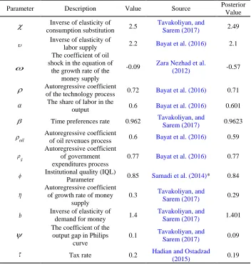
After linearizing final equations, in this section, by using DYNARE software (version 4.3.3), as well as the initial values of parameters, the final values of the parameters are estimated using a Bayesian method. Given the log-linearized form of the equations, the coefficients of variables that are in the form of deviations from the steady state values are divided into two groups. The first group is parameters of the model. Prior distribution, mean, and standard deviation of these parameters are determined by using previous studies or econometric methods. DYNARE software, by utilizing these data as well as Metropolis–Hastings algorithm, estimates the mean of posterior distribution of parameters. The results are presented in Table 1.
The second group includes such ratios as the ratio of tax revenue to the government expenditures, which are obtained using the steady state values of variables over the period under review. These calibrated ratios are given in Table 2.
5.3 Model Validation Tests
One way to check validity of the results is to check the posterior distribution. The posterior distribution should have a standardized form and should not have characteristics such as having two or more humps, skewness, i.e. be bimodal, multimodal, or skewed, or any feature that causes the distribution shape to be unusual (Tavakolian and Sarem, 2017). The results of this study showed that none of the posterior distributions had unusual (non-normal) shape; therefore, the validity of estimation of parameters was confirmed.
Table 1. Calculated Parameters of the model
Posterior Value Source
Value Description
Parameter
2.49
Tavakoliyan, and Sarem (2017)
2.5 Inverse of elasticity of
consumption substitution
2.1
Bayat et al. (2016)
2.2 Inverse of elasticity of
labor supply
-0.57
Zara Nezhad et al. (2012)
-0.09 The coefficient of oil
shock in the equation of the growth rate of the
money supply
0.71
Bayat et al. (2016)
0.72 Autoregressive coefficient
of the technology process
0.601
Bayat et al. (2016)
0.6 The share of labor in the
output
0.9623
Tavakoliyan, and Sarem (2017)
0.962 Time preferences rate
0.59
Bayat et al. (2016)
0.6 Autoregressive coefficient
of oil revenues process
oil
0.77
Bayat et al. (2016)
0.77 Autoregressive coefficient
of government expenditures process
g
0.84
Samadi et al. (2014)* 0.85
Institutional quality (IQL) Parameter
0.29
Tavakoliyan, and Sarem (2017)
0.3 Autoregressive coefficient
of growth rate of money supply
1.401
Tavakoliyan, and Sarem (2017)
1.4 Inverse of elasticity of
demand for money
b
0.09
Tavakoliyan, and Sarem (2017)
0.1 The coefficient of the
output gap in Philips curve
0.19
Hadian and Ostadzad (2015)
0.2 Tax rate
Table 2. Calculated Ratios
Ratio T/G d/G m/G G/y c/y i
Descr iption Ratio of steady tax revenue to government expenditures
The ratio of the steady form of participation bonds to government expenditures
The ratio of steady monetary
base to government expenditures
The ratio of steady state- to-production expenditures Relative mode of consumption to production Steady rate of interest rate
value 0.9 0.7 1.2 0.77 0.9 0.041
Source: Research Finding
In DYNARE software, the Brooks - Geleman Diagnostics test is graphically depicted in form of two, a blue and a red, lines. In this diagram, the red line represents the intra-chain variance, i.e. the within block variance, and the blue line represents sum of the within and between block variances. Therefore, validity of Bayesian's estimate is confirmed if these two lines converge together (Tavakolian and Sarem, 2017). The result of Brooks - Geleman Diagnostics test is presented in Appendix for all of the parameters.
5.4 Calculation of the Coefficient of Optimal Monetary Policy over a Business Cycle
After doing mathematical calculations, we arrived at the relationship
t yt
with regard to optimal monetary policy during business cycles, where
) 1 ( l l
. Here, ,l denote the weight of the government expenditures gap
and output gap in the policy maker's loss function, respectively. , and
stands for the tax rate, the output gap in the Philips curve, and institutional quality, respectively. Considering that all parameters are positive, the optimal behavior of monetary policy during business cycles is countercyclical. To obtain
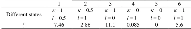
value, the parameters need to be located. The parameters , , are calculated by using a DSGE framework. The values obtained for them are 0.19, 0.09 and 0.84 respectively. For ,l, following Farazmand et al. (2013), different values of 0, 1, and 0.5 are used to compare the optimal monetary policy during business cycles in different states (modes). The result of this comparison is reported in Table 3:Table 3. The coefficient of optimal monetary policy during business cycles in different states 6 5 4 3 2 1 1 1 l 0 0 l 1 0 l 0 1 l 1 5 . 0 l 5 . 0 1 l Different states 5.6 0 0.085 11.1 2.86 7.46
It can be seen from Table 3:
- First state: If the weight of output gap is twice that of government's expenditures gap, the optimal monetary policy will be countercyclical with a relatively large coefficient (equal to 7.46). This is quite expected because when a policymaker puts the great importance on stabilizing output, he will have a great desire to adopt countercyclical monetary policies.
- Second state: if fiscal dominance in the economy is high, so that the weight of the expenditures gap is twice that of output gap, the optimal monetary policy during business cycles will have a relatively small coefficient (equal to 2.86).
- Third state: If there is no fiscal dominance in the economy and a completely independent monetary policy is adopted, in fact, the policymaker's goal is only to stabilize output and inflation, the optimal monetary policy is strongly countercyclical and has the largest coefficient (equal to 11.1).
- Fourth state: If the policymaker just considers the government's expenditures and does not place any weight on the stabilization of output, the optimal monetary policy during business cycles will be countercyclical with a very small coefficient (equal to 0.085).
- Fifth state: If none of output gap and expenditure gap is important for policy maker and the policymaker is only willing to stabilize inflation, the optimal monetary policy will be independent of the business cycles. This is consistent with Kim’s (2014) study.
- Sixth state: If the policymaker places equal weight on both output gap and expenditure gap, the optimal monetary policy coefficient will be equal to 5.6 and is placed between the first and the second states.
5.4 Sensitivity Analysis
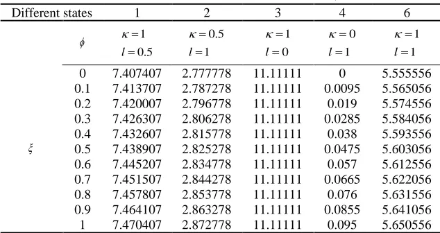
In section 4.4, the coefficient of optimal monetary policy during business cycles in different states is calculated. In fact, for different values of ,l, behavior of monetary policy is investigated. Here we consider different value of institutional quality (IQL) parameter that is between 0 to 1 and calculate the coefficient of optimal monetary policy during business cycles () in different states. Table 4 shows the result.
Table 4. Sensitivity analysis of the coefficient of optimal monetary policy during business cycles in different states relative to.
6 4 3 2 1 Different states 1 1 l 1 0 l 0 1 l 1 5 . 0 l 5 . 0 1 l 5.555556 0 11.11111 2.777778 7.407407 0 5.565056 0.0095 11.11111 2.787278 7.413707 0.1 5.574556 0.019 11.11111 2.796778 7.420007 0.2 5.584056 0.0285 11.11111 2.806278 7.426307 0.3 5.593556 0.038 11.11111 2.815778 7.432607 0.4 5.603056 0.0475 11.11111 2.825278 7.438907 0.5 5.612556 0.057 11.11111 2.834778 7.445207 0.6 5.622056 0.0665 11.11111 2.844278 7.451507 0.7 5.631556 0.076 11.11111 2.853778 7.457807 0.8 5.641056 0.0855 11.11111 2.863278 7.464107 0.9 5.650556 0.095 11.11111 2.872778 7.470407 1
Source: Research Finding
The coefficient of optimal monetary policy in third state is constant for all values of. It is because we consider institutional quality in fiscal sector, since in this state that there is no fiscal dominance, therefore IQL parameter has not effect.
For the first, second and sixth states, changes of
due to changes of are small. Although in all these states, by improving IQL parameter(
),
becomes
larger. That means countercyclical behavior of monetary policy becomes stronger.6. Conclusion
Despite the fact that countercyclical monetary policy is considered as the optimal monetary policy during business cycles by most of the economists, the questions of “What is the optimal monetary policy during the business cycles?” and “Is still countercyclical monetary policy an optimal policy?” when a developing country like Iran suffers from weak institutional quality and fiscal dominance policy remain unanswered
To find the answers to these questions, this study used a New Keynesians DSGE model in accordance with Iran's economic structure. Taking into account the roles of institutional quality and government fiscal dominance, the optimal monetary policy during the business cycle was derived.
model parameters were calculated in a DSGE framework and by using a Bayesian method. Validity of the estimated parameters was assessed using the MCMC Brooks-Gelman diagnostics. Next, these parameters were used to calculate the coefficient of optimal monetary policy during business cycles.
The coefficients of the optimal policy for different weights on government expenditures and on output were calculated and compared. The results of the study show:
- The optimal monetary policy during business cycles even with inclusion of institutional quality and fiscal dominance is countercyclical.
- Improvement in institutional quality enhances the stabilizing capability (strength) of countercyclical monetary policy.
- Fiscal dominance makes the coefficient of optimal cyclical policy smaller.
- The most effective stabilizing capability of countercyclical policy takes place when monetary policy is fully independent.
- When the policymaker's goal is merely to stabilize prices, optimal cyclical monetary policy is acyclical.
In the end, according to the results obtained, we suggest:
- Policymaker should provide conditions to implement countercyclical monetary policy, so that in the periods of recession and expansion (boom) he/she can reduce economic fluctuations by pursuing appropriate policies.
- Policymaker should increase the independence degree of the Central Bank.
References
Bayat, M., Afshari, Z., & Tavakoliyan, H. (2017). Monetary policy and total
index of stock price within the framework of a DSGE model. Quarterly
Journal of Economic Research and Policy, 3(78), 178-206.
Calderon, C., Duncan, R., Schmidt-Hebbel, K. (2012). Do good institutions
promote counter-cyclical macroeconomic policies? Oxford Bulletin of
Economics and Statistics, 78(5),650-670.
Duncan, R. (2014). Institutional quality, the cyclicality of monetary policy and
macroeconomic volatility, Journal of Macroeconomics, 39, 113–155.
Farazmand, H., Ghorbanzhad, M., & Pourjavan, A. (2013). Determining the
rules of optimal monetary and fiscal policies in Iran's economy. Quarterly
Journal of Economic Research and Policy, 67, 69-88.
Frankel, J., Vegh, C. A., & Vuletin, G. (2011). Fiscal policy in developing countries: Escape from procyclicality.
http://www.voxeu.org/article/how-developing-nations-escaped-procyclical-scal-policy.
Gruben, W. C., & Welch, J. H. (2010). Is tighter fiscal policy expansionary under fiscal dominance? Hyper crowding out in Latin America,
Contemporary Economic Policy, 28(2), 171-181.
Hadian, I. & Ostadzad, A. H. (2015). Calculation of the optimal rate of income
tax with and without environmental considerations. Quarterly Journal of
Applied Economic Studies of Iran, 24, 1-25.
Huang, H. & Wei, S. J. (2006). Monetary policies for developing countries: the
role of institutional quality, Journal of International Economics, 70, 239–
252.
Kim, J. (2014). Cyclicality of optimal stabilization policy in developing countries under frictions: Role of imperfect infrastructural development,
Discussion Paper in Economics, Colorado University, 13-11.
Motevaseli, M., Ebrahimi, A., Shahmoradi, A., & Tajik, A. (2010). Design a New Keynesian dynamic stochastic general equilibrium model for the
economy as an exporter of oil. Quarterly Journal of Economic Research,
(4), 116-87.
Rahmani, T. & Yousefi, H. (2008), Corruption, monetary policy, and
cross-country examination, www.dmk.ir/Dorsapax/userfiles/file/Corruption, 1-18.
Samadi, A. H., Marzban H. & Sajedianfard, N. (2014). Tax evasion, effective tax rate and economic growth in Iran: an endogenous growth model.
Proceedings of the 8th Conference on Iranian Tax and fiscal policies,
Tehran.
Taqavi, M., & Safarzadeh, A. (2009). The optimal rate of growth of liquidity in the economy in the context of New Keynesian dynamic stochastic general
equilibrium models. Quarterly Journal of Economic Modeling, 3 (3),
Tavakoliyan, H., & Sarem, M. (2017). DSGE models in DYNARE Software,
Modeling, Solving and Estimating based on Iranian Economy. Tehran,
Banking and Monetary Research Center.
Végh, C., A., & Vuletin, G. (2012). The Road to redemption: policy response to
crises in Latin America, IMF Economic Review, Palgrave Macmillan,
62(4), 526-568.
Walsh, C. (2010). Monetary Theory and Policy. (3rd Edition). Massachusetts
Institute of Technology Press.
Yakhin, Y. (2008). Financial integration and cyclicality of monetary policy in
Small open economies, Manuscript, Rice University.
Zara Nejad, M., & Anvari, A. (2012). Determine the optimal monetary and fiscal policy uncertainty in the economy with micro foundation of
macroeconomic model. Journal of Monetary and Financial Economics, (3),
Appendix
MCMC result for all parameters: