3D vortex simulation of flow in an opposed-piston engine

(1)

161

3D Vortex Simulation of Flow in An Opposed-Piston Engine

Adrin Gharakhani† and Ahmed F. Ghoniem‡

†

Applied Scientific Research, USA, E-mail: [email protected] ‡

Massachusetts Institute of Technology, USA, E-mail: [email protected]

Abstract

A 3-D Lagrangian random vortex-boundary element method is extended to the case of compressible flow at low Mach numbers. The simulations utilize the equation for the transport of (vorticity/density), which is identical in form to the vorticity transport equation for incompressible flow, but with two modifications. First, diffusion involves a time-varying, spatially homogeneous diffusivity. This is implemented by appropriately modifying the diffusion time scale, so that the diffusivity is time-invariant. Second, the continuity equation includes a spatially uniform, but time-dependent density. This effect is accounted for in the potential component of the velocity field via a Poisson equation with a spatially-uniform, time-dependent volumetric source term. The latter is converted to a source on the boundary of the domain, which allows the grid-free evaluation of the potential velocity field using the boundary element method. As a result, grid-free simulation of flow in the complex geometry of engines during the entire intake and compression strokes is made possible. In this paper, the formulation for the method and preliminary results from the simulation of the swirling flow inside a typical two-stroke opposed-piston engine are presented.

Introduction

A 3-D random vortex-boundary element method was developed recently for the grid-free simulation of the intake flow in internal combustion engines [8]. In this approach, the surface of the engine was defined in terms of a set of rectangular and/or triangular elements. The elements were used with the boundary element method to solve a Neumann problem that imposes the normal flux boundary condition. They were also used to generate vorticity on the engine solid walls to satisfy the no-slip boundary condition. The evolution of the flow field was predicted by the Lagrangian transport of the vorticity field using the vortex elements that originate at the walls. The detailed formulation of the vortex-boundary element method and a parametric test of its accuracy were given in [7].

In this paper, we extend the random vortex-boundary element method and present an approach for predicting the flow in engines during the compression stroke. The formulation of the method is based on the assumption that the flow in engines is primarily in the low Mach number limit, which implies that, to the leading order, the pressure in the engine is a function of time only [10-12]. Furthermore, neglecting small temperature gradients near the walls, the density is also taken to be a function of time. This results in a transport equation for (vorticity/density) which is identical in form to that for the vorticity with two exceptions. (1) The effective Reynolds number in the new formulation is time-dependent, because the kinematic viscosity is a function of the temperature and thus time. (2) The continuity equation includes a compressibility effect, which manifests itself as a spatially-uniform, time-varying density. In this paper, we show that the time-dependent Reynolds number may be incorporated into the effective time of a new diffusion equation that has a constant Reynolds number, which can then be solved using conventional methods. We also demonstrate that the time-derivative of the density, which acts as a uniformly distributed volumetric source term, is equivalent to the surface distribution of a new source term. This facilitates the effective use of the boundary element method for evaluating the potential flow field while preserving the grid-free nature of the computations.

(2)

In what follows, we present the random vortex-boundary element formulation for compressible flow at the low Mach number limit. We also present preliminary results from the simulation of flow inside a typical two-stroke opposed-piston engine during the compression stage.

1 Formulation

The equations of motion, energy and state of an ideal gas flow in an engine at the low Mach number limit may be approximated as

Dρ Dt +ρ

&

∇ ⋅u &=0 (1a)

ρDu &

Dt = −

&

∇ p+ 1 Re

&

∇ ⋅σ +& O Ma

( )

2 _(1b)

ρDT

Dt − γ − 1

γ

dp dt = −

1 Pe

&

∇ ⋅q &+O Ma

( )

2

(1c)

p=ρT (1d)

is the velocity vector normalized by a characteristic speed, U; t is the time normalized by L U ; p, ρ and T are the pressure, density and temperature normalized by

po, ρo and To at some reference time, respectively; γ is the specific heat ratio;

&

σ and q are the shear stress& tensor and the conductive heat flux vector, respectively; Ma=U γ po ρo, Re=UL νo and Pe=UL αo are

the Mach, Reynolds and Peclet numbers, respectively; and νo and αo are the kinematic viscosity and the

thermal diffusivity at some reference time, respectively.

Equations (1b) and (1c) were derived using an expansion of the u , p and T variables in the Mach number Ma& [10-12]. The expansions yield ∇ &p≈0 to zeroth order; meaning that, to the leading order, the pressure is equalized instantaneously throughout the engine chamber and is thus a function of time only, p≈ p t

( )

. Furthermore, higher order expansions indicate that, up to O Ma

( )

2 , the momentum and the energy equations

are decoupled so that their solutions can be obtained sequentially rather than simultaneously.

In this paper, we consider the fluid dynamics of pre-combustion compression in engines, during which the fluid density is spatially uniform (neglecting small changes in the temperature near the walls). The vorticity transport formulation for the flow in a three-dimensional domain D, with boundary surfaces ∂D , is derived by taking the curl of (1b) and substituting (1a). The resulting equations are

DΩ & Dt =

&

Ω ⋅∇ &u &+ ν Re∇

2&

Ω x &∈D (2a)

&

∇ ⋅u &= −1

ρ

dρ dt

&

x ∈D (2b)

&

(3)

&

ω =∇ &∧_u& _x&_∈_D _(2d)

&

u

(

&x , t

)

=

(

u &⋅τ &,u &⋅ρ &,u &⋅n &

)

x &∈∂D (2e)

&

u

(

&x , t=0

)

=u &o

&

x ∈D (2f)

where ω &

(

&x , t

)

=

(

ωx,ωy,ωz

)

is the vorticity vector normalized by U L ; ν and V are the kinematic viscosity and

, it changes as Re ν at subsequent times. Second, conservation of mass, written is terms of the velocity divergence, has a source term. Thus, the potential flow component is governed by a Poisson equation with a spatially uniform source term, instead of a Laplace equation as in the incompressible flow case.

Vorticity is discretized by NV vortex elements defined by their volume ∆Vi, vorticity

&

ω i, and center

&

x i

&

ω

(

&x , t

)

= Γ &i

( )

t gσ

&

x −x &i

(

)

j=1

NV

∑

(3)

where gσ

(

&x

)

= 1

σ3g

& x σ     

 is a spherical core function with radius σ, and Γ &i

( )

t =

&

ω i

( )

t∆Vi is the volumetric

vorticity. We used g

(

x &

)

= 3

4π 1−tanh

2 & x 3

( )

[

]

from [3]. Given the above vorticity field and subsequent to the application of viscous splitting [2], the discrete Lagrangian form of Eqs. (2) can be integrated in time as:

&_′

χ i

( )

tk+1 =

&

χ i

( )

tk +F

&

u i

&

χ i, tk

(

)

[

]

∆t (4a)

&

[

]

∆t (4b)

&

χ i

( )

tk+1 =

&_′

χ i

( )

tk+1 +

&

η i (4c)

&

χ i

( )

to =

&

χ i,o

&

Γ i

&

χ i, to

(

)

=Γ &i,o k=0,1,... i=1, ..., NV

where χ &i describes the trajectory of the i-th vortex element originating from

&

χ i,o with volumetric vorticity

&

Γ i,o,

to is the time it is introduced into the domain, ∆t=

(

tk+1−tk

)

is the integration timestep, and F

[]

⋅ represents

the time integration scheme. We used the second-order modified Euler method. Equation (4c) is the random walk solution of the diffusion equation and η &i =

(

ηx,ηy,ηz

)

(4)

Gaussian distribution. We will discuss the diffusion equation shortly.

1.1 The Velocity Field

The velocity and its gradients at the center of the elements are evaluated as the sum of a vortical field in free space and a potential flow that imposes the normal flux boundary condition. The discrete regularized vortical velocity and its gradients are evaluated as follows [1]:

&

u ω

( )

&x i,t = Kσ

&

x i−

&

x j

(

)

∧&

Γ j

( )

t j=1

N_V

∑

(5a)

i=1, ..., NV

&

∇ u &ω

( )

&x i, t =

&

∇ Kσ x &i−

&

x j

(

)

∧&

Γ j

( )

t j=1

N

V

∑

3 .

The potential component of the velocity and its gradients are evaluated subsequent to the solution of the following three-dimensional Poisson equation for the interior:

∇2

Φ

(

x &

)

= −1 V

dV dt = −

Si

&

u i⋅

&

n

i

∑

V = −ε

( )

t

&

x ∈D (6a)

q

( )

x &o = −

&

is the unknown potential, the gradient of which yields the potential velocity, u &P

&

x

(

)

= −∇ Φ&

(

x &

)

, and q

( )

x &o is its normal flux at the boundary. Si and

&

u i are the areas and velocities of the surfaces defining the

engine, respectively. Equations (6) may be reformulated in terms of a boundary integral equation:

α

(

x &

)

Φ

(

x &

)

= q

( )

&x o G

&

x ,x &o

( )

− Φ

( )

x &o

&

∇ G

(

x ,& x &o

)

⋅

&

n

[

]

dS

( )

&x o

&x ,x &o∈D (6c)

where G

( )

&x ,&x o =

x &

)

= q

( )

x &o + ε

t

( )

2

&

x −&x o

(

)

⋅n &

 

  _ G

( )

&

x i

(

)

εjpl τl kΦ

k ,ρ

( )

&x o − ρl kΦ

k,τ

( )

&x o

[

]

+ δjpqk

&

x o

( )

{

}

dSk

&

x o

( )

∂D_k

∫

k₌1

M

∑

+ ε

( )

tG &x o,

&

x i

(

)

nj k

dSk

&

x o

( )

∂Dk

∫

k₌1

M

∑

(8a)

∂u_P

j

&

x _i

( )

∂x_m = G, p

&

x o,

&

x i

(

)

εjpl

τl kρ m kΦ k,ρρ &

x _o

( )

−ρl kτ

m kΦ

k,ττ

&

x _o

( )

+ τl

kτ m k −ρ

∫

k=1

M

∑

+ G, j

&

x o,

&

x i

(

)

τm k

qk ,τ

( )

x &o +ρm k

qk,ρ

( )

x &o −nm k

Φk,ττ

( )

x &o + Φk,ρρ

( )

&x o

(

)

[

]

dSk

&

x o

( )

∂D_k

∫

k₌1

M

∑

− ε

( )

t G, m

&

x o,

&

x i

(

)

nj k

+G, j

&

x o,

&

x i

(

)

nm k

[

]

dSk

&

x o

( )

∂Dk

∫

k=1

M

∑

(8b)

j ,l , m, p

(

)

=1, 2,3 i=1, ..., NV

where j, l, m and p indices indicate direction with respect to the global coordinate system and follow the Einstein rule, εjpl is the permutation tensor, and

()

⋅,r represents differentiation with respect to

&

x o in the r-th

direction. M is the total number of boundary elements. Note that the last terms in Eqs. (8a-8b) are the contributions of compressibility on the velocity field and its gradients, which have been formulated here in terms of regularized surface integrals.

1.2 The Diffusion Field

The diffusion sub-step of the Navier-Stokes equations is

∂Ω & ∂t = νRe∇

2Ω & _x&∈_D

(9)

which upon appropriate rescaling of the time variable may be reformulated into a diffusion equation with constant Reynolds number:

∂Ω & ∂_tˆ =

1 Re∇

2Ω & _x&∈_D _(10a)

∆_tˆ ₌_tˆ

k+1−ˆ t k = νdt tk

t_k₊₁

∫

k=0,1,... (10b)

(6)

independent random variables selected from a Gaussian distribution with zero mean and variance equal to 2∆t Re . Equation (10b) is evaluated with second order accuracy in time using the mid-point rule. Thus, theˆ

variance is 2ν ∆t Re and ν = ν

[

( )

tk +ν

( )

tk+1

]

2 .

1.3 The Boundary Region

Substantial extensions have been introduced to Chorin’s scheme [4, 5] for simulating the processes of vorticity generation to satisfy the no-slip boundary condition, and evolution within a thin region near the engine walls. First, a formulation has been developed that uses triangular, rather than rectangular, vortex tiles to discretize the surface vorticity, which provides the flexibility to simulate the flow in arbitrarily complex geometries [8]. Second, the vorticity transport approximations for the thin near-boundary layer are modified to account for low Mach number compressibility effects [9]. This includes a provision for the change in the numerical boundary layer thickness to accommodate the change in the Reynolds number due to compression or expansion. In the interest of brevity of presentation we refer the reader to [9] for the details of the formulation.

2 Results

Preliminary results from the simulation of the scavenging (intake/exhaust) and compression processes inside a “two-stroke opposed-piston engine” are presented. The objective here is to demonstrate, for the first time, the feasibility of simulating the flow inside a highly complex, time-dependent geometry of interest to industrial applications using the 3-D vortex-boundary element method. The ultimate goal is to use such simulations in a parametric study to optimize the engine design with respect to a set of objectives. We use the results to shed some light on the complexity of the developing flow.

(7)

For the purpose of this simulation, all dimensions were normalized with respect to the cylinder diameter, Dc.

The velocity was normalized with respect to the maximum piston speed, Vm, at mid-stroke. The pistons

traveled with the same amplitude and period of oscillation, but were 12 degrees out of phase. The crank angles (which are time indicators) were referenced to the lower piston; e.g., the bottom-dead center of the lower piston was reached at 180 degrees while the top-dead center of the upper piston was reached 12 degrees later, at 192 degrees. The stroke length for both pistons was 1.231. Minimum and maximum piston-to-piston separations were 0.064 and 2.512, corresponding to six and 186 degrees crank angle, respectively. The engine geometry was time-varying and, depending on the crank angle, consisted of three distinct computational topologies: (1) the cylinder was bounded by the two pistons, in which case all the walls were solid; or (2) the intake ports were in the fully open position; or (3) the intake ports were partially open at the intersections of the intake ports with the cylinder walls (Figures 1 and 2). The opening/closure of the exhaust ports did not change the engine topology in the computational sense. The height and the total area of the intake ports, at the cylinder wall, in the fully open position were 0.191 and 0.482, respectively. The corresponding values for the exhaust ports were 0.284 and 0.714, respectively. The intake normal flux boundary condition was set to be spatially uniform, but time dependent and a function of the port opening at the port-chamber interface (which is partially masked by the piston during part of the operation). The magnitude of the inlet normal velocity varied from zero to 10.7. The exhaust normal velocity was assumed to be constant in time and was assigned uniformly at 3.14 across the opening at the chamber wall. These values were either provided through experimental measurements or based on estimates related to the operation of the engine. The instantaneous volumetric source term was obtained via Eq. (6a) to balance out the net mass flux into the engine, taking the motion of the pistons into consideration.

The reference kinematic viscosity, νo, and engine volume, Vo, were assigned at 186 degrees – the maximum

piston-to-piston separation. The Reynolds number based on Dc, Vm andνo was set to 500. Note that the

time-dependent Reynolds number was equal to 500 at 186 degrees only; however, it increased subsequently due to the decrease in the value of viscosity during compression, which was approximated as an isentropic process. The full stroke was discretized using 400 equal timesteps, corresponding to ∆t=0.0097 . The maximum allowable surface vorticity for the wall-generated tiles was set to 0.5. The near-boundary layer thickness was set to 1.5 2ν ∆t Re , which was a maximum at 186 degrees but decreased thereafter during compression. The number of triangular boundary elements, used to solve the potential flow problem, ranged from 1,152 to 7,448. The corresponding number of collocation points ranged from 578 to 3,746. The number of triangular tiles, used to impose the no-slip boundary condition at the solid walls, ranged from 242 to 1,338. The total number of vortex elements in the domain peaked at 113,904. The code was parallelized efficiently via MPI to reduce the wall clock time by 1-2 orders of magnitude compared to a single-processor computation (using up to 256 processors). Note that the resolutions of the wall boundary elements and the vortex tiles were rather low. As such, we expect to be able to capture the large scales of the flow only, and to draw qualitative conclusions with regard to the flow dynamics in this complex, time-dependent geometry. Nonetheless, the results, as will be shown, are insightful and sufficient for demonstrating the advantages of the method and some of the basic features of the underlying flow.

(8)

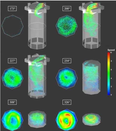
the vortex elements, which are depicted as solid circles. Showing the vortex elements introduced via a single port is necessary in order to delineate the flow in the cylinder. As expected, and during most of the stroke, the same flow pattern is observed from all ports.

Figure 1 clearly shows a strong helical motion which is imparted on the incoming jet as it moves into the cylinder. This is due to the combined action of the swirl created by the tangential jet entry, and the axial motion induced due to the piston descending towards the bottom of the cylinder. The incoming jets are seen to (radially) disperse and merge together into an effective leading front that encompasses the chamber cross-section and “sweeps” the existing fluid out through the exhaust ports. The plots also show that the fresh charge reaches the exhaust ports and partially leaves the cylinder before the ports are fully closed. Indeed, the leading front of the incoming flow reaches the exhaust ports just as the top piston crosses past the upper side of the inlet ports as it moves toward the chamber center. Therefore, under the conditions of this simulation, the scavenging process appears to be efficient; i.e., combustion products from the previous cycle are expected to be displaced effectively through the exhaust ports and the compression process is expected to involve mostly fresh charge.

The analysis of the dispersion and merging of the neighboring jets in the engine is complicated by their apparent stratification into multiple distinctly identifiable helical braids in the chamber, each interacting with similar braids from the other ports (Figure 1 - 200 and 227 degrees crank angle). Multiple braids develop because the size of the intake port opening at the port-chamber interface changes as the piston traverses across it, and because the flux and angular momentum of the fresh charge into the cylinder vary in time. A qualitative description of this process is attempted here. During the scavenging process, as the upper piston travels toward its top dead center and the intake port just opens, the incoming jet at the chamber top is directed downward at approximately 45 degrees with respect to the horizontal. Furthermore, because the intake flux is small when the port just opens, the momentum is too weak for the jet to penetrate the chamber tangentially; instead, it expands in the radial direction. This is verified by the tail ends of the jets at 173 degrees in Figs. 1 and 2, which are clearly positioned proximal to the axis of symmetry of the chamber rather than its periphery. Note that the angle of the jet with respect to the cylinder axis is primarily determined by the geometry of the intake port and the flow inside it. As the upper piston reaches its top dead center, the intake port becomes fully open and the jet issues into the chamber parallel to the piston face. At this stage, the incoming jet momentum reaches its peak and the jet penetrates tangentially into (and around the circumference of) the chamber, with very little radial expansion. In between these two limits, the jet shifts its vertical orientation from 45 degrees to zero with respect to the horizontal, and its horizontal penetration from a "fully" radial to a "fully" tangential orientation - while simultaneously increasing its speed at the inlet from zero to its peak at 10.7. Note that the reverse process takes place while the upper piston changes course and travels from the top dead center toward its bottom. This "fanning" of the jets across the entire chamber cross-section is significant for effective scavenging. Furthermore, it is most likely an important factor affecting the mixing efficiency in the engine and needs to be investigated parametrically. Other factors which affect mixing are viscous dissipation associated with the incoming jet penetration into the exhaust gas, and the boundary layers on the cylinder walls.

(9)

"compartmentalization" of the kinetic energy in the upper half of the cylinder and the precessing of the vortex center will have a detrimental effect on selecting the vertical position, the timing and the duration (and perhaps frequency) of fuel injection in the chamber; and thus on combustion stability and efficiency. For example, injecting fuel in "dead zones" will lead to poor mixing and inefficient combustion.

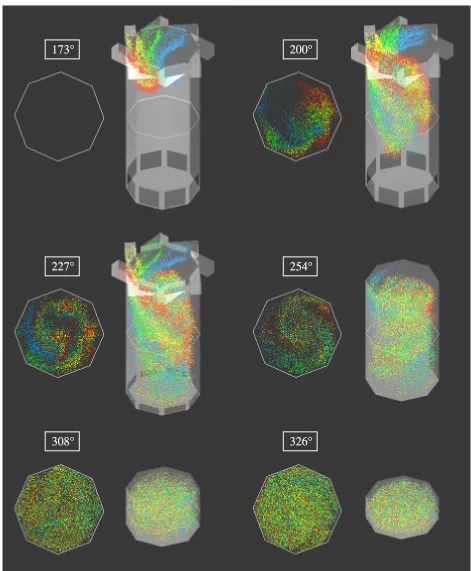
Figure 2 depicts the top and perspective views of the trajectory of the vortex elements issuing from four consecutive ports, at selected crank angles. The top view displays the trajectories within a slice of volume with 0.05 thickness and plane of symmetry which cuts through the middle of the cylinder - identified by a thin line on the cylinder in the perspective view. The elements are color coded by the originating port to facilitate the visual inspection of the mixing efficiency of the engine. The figure shows the entrainment of fluid particles in the swirling motion and their full mixing at the end of compression, as verified by the near homogeneous distribution of colors in the engine at later stages.

3 Conclusions

A model, based on the transport of the (vorticity/density) variable, has been developed for the random vortex-boundary element simulation of low Mach number compressible flow in three-dimensional engines. Two complexities introduced in the new formulation were the presence of (1) a spatially uniform source term in the continuity equation and (2) a time dependent Reynolds number in the diffusion equation. (1) Regularized surface integrals were developed in conjunction with the boundary element evaluation of the influence of the source term on the potential velocity and its gradients. (2) The time dependence of the Reynolds number was incorporated in the time variable of a new diffusion equation with a constant (reference) Reynolds number, which was then solved by the standard random walk method. The new method was used to simulate the complex swirling flow inside a two-stroke opposed-piston engine. The accuracy of the model remains to be tested against a well-documented engine experiment.

Acknowledgments

This project was funded by Gas Research Institute. The numerical experiments were performed on the Cray T3E at the San Diego Supercomputing Center.

References

1 Anderson, C. and Greengard, C., “On Vortex Methods,” SIAM Journal on Numerical Analysis, 22, No. 3 (1985), 413-440.

2 Beale, J. T. and Majda, A., “Rates of Convergence for Viscous Splitting of the Navier-Stokes Equations,” Mathematics of Computation, 37, No. 156 (1981), 243-259.

3 Beale, J. T. and Majda, A., “High Order Vortex Methods with Explicit Velocity Kernels,” Journal of Computational Physics, 58 (1985), 188-208.

4 Chorin, A. J., “Vortex Models and Boundary Layer Instability,” SIAM Journal on Scientific and Statistical Computing, 1, No. 1 (1980), 1-21.

5 Fishelov, D., “Vortex Methods for Slightly Viscous Three-Dimensional Flow,” SIAM Journal on Scientific and Statistical Computing, 11, No. 3 (1990), 399-424.

(10)

Regularized Formulation for the Potential Velocity Gradients,” International Journal for Numerical Methods in Fluids, 24, No. 1 (1997), 81-100.

7 Gharakhani, A. and Ghoniem, A. F., “Three Dimensional Vortex Simulation of Time Dependent Incompressible Internal Viscous Flows," Journal of Computational Physics, 134, No. 1 (1997), 75-95. 8 Gharakhani, A. and Ghoniem, A. F., “Toward A Grid-Free Simulation of Flow In Engines,” The 1997

ASME Fluids Engineering Division Summer Meeting, FEDSM97-3025 (Vancouver, Canada, June) (1997), 1-11.

9 Gharakhani, A. and Ghoniem, A. F., “3d Vortex Simulation of Flow In Engines During Compression” The 1998 ASME Fluids Engineering Division Summer Meeting, FEDSM98-5001 (Washington, D.C., June) (1999), 1-9.

10Ghoniem, A. F., “Computational Methods in Turbulent Reacting Flow,” in Reacting Flows: Combustion and Chemical Reactors, Part 1, Lectures in Applied Mathematics, 24 (1985), 199-265.

11Majda, A. and Sethian, J., “The Derivation and Numerical Solution of the Equations for Zero Mach Number Combustion,” Combustion Science and Technology, 42 (1985), 185-205.

12Sivashinsky, G. I., “Hydrodynamic Theory of Flame Propagation In An Enclosed Volume,” Acta Astronautica, 6 (1979), 631-645.