Properties of the Bayesian Knowledge Tracing
Model
∗
BRETT VAN DE SANDE Arizona State University [email protected]
Bayesian knowledge tracing has been used widely to model student learning. However, the name “Bayesian knowledge tracing” has been applied to two related, but distinct, models: The first is the Bayesian knowledge tracingMarkov chainwhich predicts the student-averaged probability of a correct application of a skill. We present an analytical solution to this model and show that it is a function of three parameters and has the functional form of an exponential. The second form is the Baysian knowledge tracinghidden Markov model which can use the individual student’s performance at each opportunity to apply a skill to update the conditional probability that the student has learned that skill. We use a fixed point analysis to study solutions of this model and find a range of parameters where it has the desired behavior.
Additional Key Words and Phrases: Bayesian knowledge tracing, student modelling, Markov chain, hidden Markov model
1. INTRODUCTION
Since its introduction by Corbett and Anderson [1995], Bayesian knowledge
trac-ing (BKT) has been widely applied to studies of student learntrac-ing and to various
tutor systems. In addition, BKT often serves as the starting point for more
compli-cated models of learning, for example [Baker and Aleven 2008; Lee and Brunskill
2012]. Researchers have applied BKT in two distinct ways: The fullhidden Markov
model (HMM) and the associated Markov chain. The purpose of this paper is to
investigate solutions of both forms of the BKT model.
BKT predicts the probability that a student will correctly apply a skill when they
have an opportunity to apply it. Typically, this model is fit to student performance
data using either a residual sum of squares (RSS) test (sometimes described as
“curve fitting”) [Corbett and Anderson 1995] or a Maximum Likelihood test
[Par-dos and Heffernan 2010], with several studies comparing the two approaches [Baker
et al. 2011; Chang et al. 2006; Pardos et al. 2011; 2012]. For the RSS test, some
au-thors have used conjugate gradients [Corbett and Anderson 1995; Beck and Chang
2007] while other authors have used a grid search over the parameter space, or
“BKT-BF” [Baker et al. 2011], to perform the fit. Likewise, for the Maximum
∗Revised version, February 2017. The original paper labeled the two forms of BKT incorrectly
Likelihood test, the most widely used fitting technique is the Expectation
Maxi-mization (EM) algorithm [Dempster et al. 1977; Chang et al. 2006].
How does the Markov chain form arise? If an RSS test is applied to the HMM,
for each step, the predictions of the HMM are averaged over the students in the
data set. In the limit of many students, this averaging procedure reduces the HMM
to the associated Markov chain. The BKT Markov chain is simple enough that it
can be solved analytically, which we will do here. We will see that the solution, in
functional form, is an exponential. Moreover, we will see that it is, in fact, a three
parameter model. As we shall see, this explains the “Identifiability Problem” first
noted by Beck and Chang [2007].
The BKT hidden Markov model [Corbett and Anderson 1995] can be used to
determine in real time whether a student has learned a skill. The probability
that the student has learned a skill is updated by student performance at each
opportunity to apply that skill. The model has four parameters which must be
supplied externally. Although the HMM is too complicated to solve analytically,
we will use a fixed point analysis to study the behavior of its solutions. Demanding
that the model behaves in a reasonable manner leads to significant constraints on
the model parameters.
2. MARKOV CHAIN FORM
The Bayesian knowledge tracing model [Corbett and Anderson 1995] has four
pa-rameters:
—P(L0) is the initial probability that the student knows a particular skill.
—P(G) is probability of guessing correctly, if the student doesn’t know the skill.
—P(S) is probability of making a slip, if student does know the skill.
—P(T) is probability of learning the skill if the student does not know the skill.
Note thatP(T) is assumed to be constant over time.
We define stepj to be thejth opportunity for a student to apply a given skill. Let
P(Lj) be the probability that the student knows the skill at step j. According to
the model,P(Lj) can be determined from the previous opportunity:
P(Lj) =P(Lj−1) +P(T) (1−P(Lj−1)) . (1)
In this model, the probability that the student actually gets opportunityj correct
is:
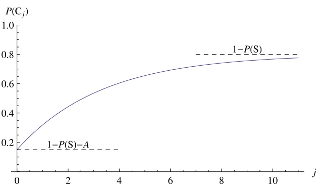
P(Cj) =P(G) (1−P(Lj)) + (1−P(S))P(Lj). (2)
Eqns. (1) and (2) define a hidden Markov model, where P(Lj) is the “hidden”
0 2 4 6 8 10 j 0.2
0.4 0.6 0.8 1.0
PHCjL
1-PHSL-A
1 -PHSL
Fig. 1. Solution of the Markov chain form of BKT, Eqn. (7). P(Cj) is the probability of the student getting stepjcorrect. Note that the solution has the functional form of an exponential.
If we interpret P(Lj) as the average value for a population of students, the
resulting Markov chain model can be solved exactly. First, we rewrite (1) in a more
suggestive form:
1−P(Lj) = (1−P(T)) (1−P(Lj−1)) . (3)
One can show that this recursion relation has solutions of the form:
1−P(Lj) = (1−P(T)) j
(1−P(L0)) . (4)
Substituting (4) into (2), we get:
P(Cj) = 1−P(S)−(1−P(S)−P(G)) (1−P(L0)) (1−P(T))j . (5)
Note that the form ofP(Cj), as a function ofj, depends on onlythreeparameters:
P(S),P(T), and (1−P(S)−P(G)) (1−P(L0)). If we define
A= (1−P(S)−P(G)) (1−P(L0)) (6)
andβ=−log(1−P(T)), then we can rewrite (5) in a clearer form:
P(Cj) = 1−P(S)−Ae−βj. (7)
Thus,P(Cj) is an exponential; see Fig. 1.
3. IDENTIFIABILITY AND PARAMETER CONSTRAINTS
The fact that the BKT Markov chain is a function of three parameters was first
0.2 0.4 0.6 0.8 1.0 PH GL 0.2
0.4 0.6 0.8 1.0
PHL0L
1
-P
H
S
L
Fig. 2. The relation between the guess rateP(G) and the initial probability of knowing a skill
P(L0) for the Markov chain associated with BKT. All points along the curve correspond to
identical Markov chains. The curve is a plot of the solutions of Eqn. (6), withP(S) = 0.05 and
A= 0.416. The three points are the three parameter sets listed in Table 1 of [Beck and Chang 2007].
In their paper, they noted that multiple combinations of P(G) and P(L0) give
exactly the same student averaged error rateP(Cj), but do not explain the origin
of these degenerate solutions. From Eqn. (6), we see that different combinations
ofP(G) and P(L0) that give the same value forAwill result in models that have
the exact same functional form. An example showing the relation between P(G)
and P(L0) for a given model is shown in Fig. 2. Thus, we can see that Eqn. (6)
provides an explanation of the Identifiability problem.
In general, for a model to make sense, all probabilities must lie between zero and
one. For the BKT Markov chain, this means that 0≤P(L0)≤1 and 0≤P(G)≤1.
If we further demand that learning is positive (which may or may not be empirically
justified), then we have the constraintA >0 orP(G)+P(S)<1. These constraints onP(L0) andP(G) correspond to the rectangular region shown in Fig. 2. In terms
ofA, valid values ofP(G) andP(L0) occur when 0 < A <1−P(S); for negative
learning, meaningful values occur when −P(S)< A < 0. This sets the range of physically meaningful values ofAwhen fitting to student data.
Note that it is reasonable for the Markov chain to find negative learning when
fitting to aggregated student data. If the students do well on the first opportunities
0.2 0.4 0.6 0.8 1.0
PHLj-1ÈOj-1L 0.2
0.4 0.6 0.8 1.0 PHLjÈOjL
step jcorrect
step jincorrect
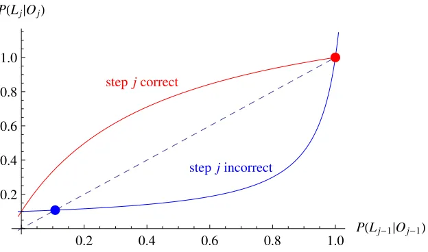
Fig. 3. Plot of the recursion relations for the BKT hidden Markov model, Eqns. (11) and (12). The
stable fixed point for each equation is marked by a dot. The dashed line represents the boundary
between increasing and decreasing solutions. Since the “stepjcorrect” curve is above the dashed line, Eqn. (11) causes the sequence{P(Lj|Oj)}to converge to the fixed point at 1. Likewise,
since the “stepj incorrect” curve is below the line, Eqn. (12) causes the sequence{P(Lj|Oj)}
to converge to the lower fixed point. The model parameters are P(S) = 0.05, P(G) = 0.3,
P(T) = 0.1, andP(L0) = 0.36.
student data will be a decreasing function, which corresponds toA <0. However, we will see that such model parameters are problematic when used as input for the
hidden Markov model.
4. HIDDEN MARKOV MODEL
In order to predictP(Lj) for an individual student in real time, the forward
algo-rithm may be employed. In this case, we find P(Lj|Oj), the probability that the
student has learned a skill just after completing stepj given student performance Oj on previous steps, where Oj ={o1, . . . , oj} is the student performance on the
first j opportunities and oi can be either correct or incorrect. This conditional
probability obeys the recursion [Baker et al. 2008]:
P(Lj−1|Oj) =
P(Lj−1|Oj−1) (1−P(S))
P(Lj−1|Oj−1) (1−P(S)) + [1−P(Lj−1|Oj−1)]P(G)
,
oj = correct (8)
P(Lj−1|Oj) =
P(Lj−1|Oj−1)P(S)
P(Lj−1|Oj−1)P(S) + [1−P(Lj−1|Oj−1)] (1−P(G))
,
oj = incorrect (9)
These equations can be combined to give:
P(Lj|Oj) = 1−
(1−P(T)) [1−P(Lj−1|Oj−1)]P(G)
P(G) + (1−P(S)−P(G))P(Lj−1|Oj−1)
,
oj= correct (11)
P(Lj|Oj) = 1−
(1−P(T)) [1−P(Lj−1|Oj−1)] (1−P(G))
1−P(G)−(1−P(S)−P(G))P(Lj−1|Oj−1)
,
oj= incorrect. (12)
Their functional forms are plotted in Fig. 3.
While this recursion relation cannot be solved analytically, we can learn much
about its solutions by conducting a fixed point analysis. This is a technique that is
covered in many differential equations textbooks; for example, see [Blanchard et al.
2006]. The goal of a fixed point analysis is to determine the qualitative behavior of
the sequence{P(Lj|Oj)}nj=0as a function ofj. IfP(Lj|Oj)> P(Lj−1|Oj−1), then
we know that P(Lj|Oj) increases with j. Likewise, ifP(Lj|Oj)< P(Lj−1|Oj−1),
then we know thatP(Lj|Oj) decreases withj. Thus, the boundary between
increas-ing and decreasincreas-ing solutions isP(Lj|Oj) =P(Lj−1|Oj−1), shown as the dashed line
in Fig. 3. Afixed pointis a value ofP(Lj|Oj) such that the recursion relation obeys
P(Lj|Oj) =P(Lj−1|Oj−1). In the example at hand, there are two kinds of fixed
points:
Stable fixed point. IfP(Lj|Oj) is near the fixed point, thenP(Lj|Oj) converges
to the fixed point asj increases;
Unstable fixed point. If P(Lj|Oj) is near the fixed point, thenP(Lj|Oj) moves
away from the fixed point with increasingj.
Let us apply these ideas to Eqns. (11) and (12). For Eqn. (11), we find a stable
fixed point at 1 and an unstable fixed point at
− P(G)P(T)
1−P(G)−P(S) . (13)
Similarly, Eqn. (12) has an unstable fixed point at 1 and a stable fixed point at
(1−P(G))P(T)
1−P(G)−P(S) . (14)
The two stable fixed points are plotted as dots in Fig. 3.
In order for P(Lj|Oj) to remain in the interval [0,1] for any starting value
P(L0) ∈ [0,1] and any sequence of correct/incorrect steps Oj, we need the
sta-ble fixed point (14) to lie in the interval [0,1] and the unstable fixed point (13) to
Fig. 4. Plot of the constraint on the learning rateP(T) as a function of the guess rateP(G)
and the slip rateP(S) given by Eqn. (16). Valid parameters for the BKT hidden Markov model lie in the region that is below this surface and above theP(T) = 0 plane. The vertical surface
represents the other constraintP(G) +P(S)<1, Eqn. (15); valid model parameters lie to the left
of this surface.
model parameters:
P(G) +P(S) < 1, (15)
0< P(T) < 1− P(S)
1−P(G) . (16)
If we instead choose parameters consistent with negative learning,P(S)+P(G)>1, we find that the behavior of P(Lj|Oj) becomes inverted: P(Lj|Oj) decreases for
correct steps and increases for incorrect steps.
Baker, Corbett, and Aleven [2008] discuss the need to choose model parameters
such that the forward algorithm behaves in a sensible fashion. In particular, they
point out that correct actions by the student should cause the estimate of learning
P(Lj|Oj) to increase. They define models that do not have this property to be
“empirically degenerate.” Our constraint (15) identifies precisely which models will
be “empirically degenerate.” Note that [Baker et al. 2008] impose the somewhat
In terms of the parameter space, Eqn. (16) provides a significant constraint on
allowed values of model parameters; see Fig. 4. In fact, it completely supersedes
the other constraintP(G) +P(S)<1.
Finally, the “Identifiability Problem” for the BKT hidden Markov model does
not exist, so long as there are both correct and incorrect steps. This fact can be seen
by examining Eqns. (11) and (12) where we see thatP(G) has a different functional form in the numerator of each equation. Thus, any redefinition of 1−P(Lj|Oj)
cannot be compensated for by a redefinition of other parameters in both (11) and
(12). That is, all four model parameters are needed to define the HMM.
5. CONCLUSION
In conclusion, the hidden Markov chain associated with BKT, when expressed in
functional form, is an exponential function with three parameters. The Markov
chain is obtained by averaging the HMM over students, which happens when
com-paring model predictions to student data using a RSS test. This suggests that
the use of a maximum likelihood test should be the preferred method for finding
parameter values for the BKT hidden Markov Model.
Our other result is that the functional form of the Markov chain corresponds to an
exponential, rather than a power law. Heathcote, Brown, and Mewhort [2000] argue
that learning for individuals is better described by an exponential while (as shown
in earlier studies) learning averaged over individuals is better described by a power
law function. However, this analysis was performed using mainly reaction time
(latency) for tasks that were already learned, while we are interested in the initial
acquisition of a skill. A recent study that focused on students learning physics skills
found that student learning was better explained by a power law function, even for
individual students [Chi et al. 2011]. Together, these results call into question the
practice of using the BKT to model student data. Perhaps a model that has power
law behavior would work better?
We see that the hidden Markov model itself does not suffer from the Identifiability
Problem: all four model parameters affect model behavior separately. We also
see that, for the model to behave properly, there are significant constraints on
the allowed values ofP(S),P(G), andP(T) and that parameters consistent with
negative learning are not allowed. Violations of these constraints should correspond
to the “empirically degenerate” models found in [Baker et al. 2008]. Also, it would
be interesting to apply to see how often these constraints are violated in situations
where BKT is employed, such as in the Cognitive Tutors [Ritter et al. 2007]. A
Finally, a fixed point analysis like the one that we conducted here could be applied
to more complicated models of learning, such as [Baker and Aleven 2008; Lee and
Brunskill 2012]. This may give us greater insight into the qualitative behaviors of
these models as well as constrain model parameters.
ACKNOWLEDGMENTS
Funding for this research was provided by the Pittsburgh Science of Learning Center
which is funded by the National Science Foundation award No. SBE-0836012. I
would like to thank Ken Koedinger, Michael Yudelson, and Tristan Nixon for useful
comments.
REFERENCES
Baker, R. and Aleven, V.2008. Improving Contextual Models of Guessing and Slipping with
a Truncated Training Set. InEducational Data Mining 2008: 1st International Conference on Educational Data Mining, Proceedings. UNC-Charlotte, Computer Science Dept., Montreal, Canada, 67–76.
Baker, R.,Corbett, A., and Aleven, V. 2008. More Accurate Student Modeling through
Contextual Estimation of Slip and Guess Probabilities in Bayesian Knowledge Tracing. In
Intelligent Tutoring Systems, B. Woolf, E. Ameur, R. Nkambou, and S. Lajoie, Eds. Lecture Notes in Computer Science, vol. 5091. Springer Berlin / Heidelberg, 406–415.
Baker, R. S. J. D.,Pardos, Z. A.,Gowda, S. M.,Nooraei, B. B.,and Heffernan, N. T.
2011. Ensembling predictions of student knowledge within intelligent tutoring systems. In Pro-ceedings of the 19th international conference on User modeling, adaption, and personalization. UMAP’11. Springer-Verlag, Berlin, Heidelberg, 13–24.
Beck, J. and Chang, K.-m. 2007. Identifiability: A Fundamental Problem of Student
Model-ing. InUser Modeling 2007, C. Conati, K. McCoy, and G. Paliouras, Eds. Lecture Notes in Computer Science, vol. 4511. Springer Berlin / Heidelberg, 137–146.
Blanchard, P.,Devaney, R. L.,and Hall, G. R. 2006. Differential Equations. Cengage
Learning.
Chang, K.-m.,Beck, J.,Mostow, J.,and Corbett, A.2006. A bayes net toolkit for student
modeling in intelligent tutoring systems. InProceedings of the 8th international conference on Intelligent Tutoring Systems. ITS’06. Springer-Verlag, Berlin, Heidelberg, 104–113.
Chi, M.,Koedinger, K.,Gordon, G.,Jordan, P.,and VanLehn, K.2011. Instructional Factors
Analysis: A Cognitive Model For Multiple Instructional Interventions. InProceedings of the 4th International Conference on Educational Data Mining. Eindhoven, the Netherlands.
Corbett, A. T. and Anderson, J. R. 1995. Knowledge tracing: Modeling the acquisition of
procedural knowledge.User Modeling and User-Adapted Interaction 4,4, 253–278.
Dempster, A. P.,Laird, N. M.,and Rubin, D. B.1977. Maximum Likelihood from Incomplete
Data via the EM Algorithm. Journal of the Royal Statistical Society. Series B (Methodologi-cal) 39,1 (Jan.), 1–38.
Heathcote, A.,Brown, S.,and Mewhort, D.2000. The power law repealed: The case for an
exponential law of practice.Psychonomic Bulletin & Review 7,2, 185–207.
Lee, J. I. and Brunskill, E.2012. The Impact on Individualizing Student Models on Necessary
Practice Opportunities. In Proceedings of the 5th International Conference on Educational Data Mining. Chania, Greece, 118–125.
Pardos, Z. A.,Gowda, S. M.,Baker, R. S.,and Heffernan, N. T.2012. The sum is greater
than the parts: ensembling models of student knowledge in educational software.ACM SIGKDD Explorations Newsletter 13,2 (May), 37–44.
Pardos, Z. A.,Gowda, S. M.,Baker, R. S. J. d.,and Heffernan, N. T.2011. Ensembling
Pardos, Z. A. and Heffernan, N. T.2010. Navigating the parameter space of Bayesian Knowl-edge Tracing models: Visualizations of the convergence of the Expectation Maximization al-gorithm. In Proceedings of the 3rd International Conference on Educational Data Mining. Pittsburgh, PA.
Ritter, S.,Anderson, J. R.,Koedinger, K. R.,and Corbett, A. 2007. Cognitive Tutor: