PhD Dissertation
International Doctorate School in Information and Communication Technologies
DIT - University of Trento
Efficient Solving of the Satisfiability
Modulo Bit-Vectors Problem and Some
Extensions to SMT
Anders Franz´en
Advisor:
Alessandro Cimatti
FBK-irst
Co-Advisor:
Roberto Sebastiani
Universit`a degli Studi di Trento
Abstract
Decision procedures for expressive logics such as linear arithmetic, bit-vectors, uninterpreted functions, arrays or combinations of theories are becoming increasingly important in various areas of hardware and software development and verification such as test pattern generation, equivalence checking, assertion based verification and model checking.
In particular, the need for bit-precise reasoning is an important target for research into decision procedures. In this thesis we will describe work on creating an efficient decision procedure for Satisfiability Modulo the Theory of fixed-width bit-vectors, and how such a solver can be used in a real-world application.
We will also introduce some extensions of the basic decision procedure allowing for optimisation, and compact representation of constraints in a SMT solver, showing how these can be succinctly and elegantly described as a theory allowing for the extension with minimal changes to SMT solvers.
Keywords
Contents
1 Introduction 1
1.1 Contribution. . . 3
1.2 Acknowledgements . . . 4
1.3 Overview. . . 4
2 Preliminaries 7 2.1 SAT . . . 7
2.2 Solving the SAT problem . . . 9
2.3 Satisfiability Modulo Theories . . . 10
2.4 Fixed-width bit-vectors . . . 11
2.5 Approaches to SMT. . . 13
2.5.1 Eager encoding into SAT . . . 13
2.5.2 Lazy encoding . . . 13
2.6 DAG representation of formulae . . . 16
2.7 MathSAT . . . 17
2.7.1 Preprocessing . . . 18
2.7.2 The solver proper . . . 19
2.7.3 Theories . . . 19
2.7.4 API . . . 20
2.7.5 Performance . . . 20
3 Solving techniques 23
3.1 Bit-blasting . . . 23
3.2 DPLL(T) or the lazy schema . . . 24
3.2.1 Bounded SAT reasoning . . . 26
3.2.2 Deduction . . . 27
3.3 Eager encoding to SAT . . . 27
3.3.1 Implementation issues . . . 27
3.4 Theory solver layering . . . 28
3.5 Static learning . . . 29
3.6 Clustering . . . 29
3.7 Minimal model enumeration . . . 31
3.7.1 Sign-Minimal Models . . . 32
3.7.2 Minimality for Standard Dual Rail . . . 33
3.7.3 Minimality in SMT . . . 33
3.7.4 Encoding of non-CNF formulae . . . 33
3.7.5 Redundancy . . . 34
4 Preprocessing 37 4.1 Normal form computation . . . 38
4.1.1 A simple rule language . . . 42
4.1.2 Rule verification . . . 43
4.1.3 Termination . . . 45
4.1.4 Implementation issues . . . 46
4.2 Substitution/variable elimination . . . 46
4.3 Combining normal forms and substitution . . . 47
4.4 Propagation of unconstrained terms and formulae . . . 48
4.5 Disjunctive partitioning . . . 51
4.6 Packet splitting . . . 53
4.8 Other techniques . . . 56
4.9 Model computation . . . 57
4.10 Incrementality and backtrackability . . . 62
4.11 Architecture . . . 64
5 Approximation of formulae 65 5.1 Over-approximation . . . 68
5.1.1 Refinement . . . 69
5.2 Under-approximation . . . 71
5.2.1 Refinement . . . 72
5.2.2 Under-approximation in theory solver . . . 73
5.2.3 Model computation . . . 74
5.3 Combining multiple approximation/refinement loops. . . . 75
6 Experimental evaluation 77 6.1 Cumulative distribution functions . . . 78
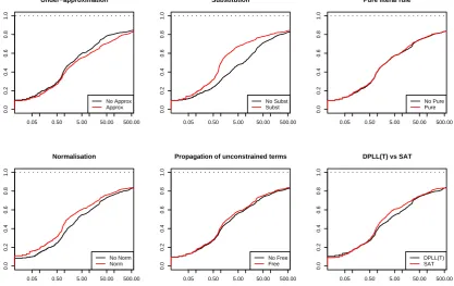
6.2 Effects of techniques . . . 79
6.3 SAT vs DPLL(T) . . . 82
6.4 Under-approximation . . . 83
6.5 Minimal model enumeration . . . 85
6.6 Core rewriting and disjunctive partitioning . . . 86
6.7 Packet splitting . . . 87
6.8 Difference propagation . . . 88
6.9 Clustering . . . 89
6.10 Comparison with other solvers . . . 91
6.11 Model computation . . . 95
6.11.1 Other solvers . . . 97
7 An industrial case study 101
7.1 Intermediate Representation Language . . . 103
7.2 Symbolic execution of microcode . . . 105
7.2.1 Some improvements to the basic symbolic execution algorithm . . . 108
7.3 Focus of this work. . . 109
7.4 Reuse of learnt information . . . 111
7.5 Unsatisfiable cores for result caching . . . 114
7.6 Non-singleton sets . . . 116
7.6.1 An alternative MSPSAT algorithm . . . 117
7.7 Basic parallelism . . . 118
7.8 Experimental evaluation . . . 119
7.8.1 Reuse of information . . . 121
7.8.2 Non-singleton sets . . . 124
7.8.3 Parallelism. . . 127
7.8.4 Unsatisfiable cores . . . 129
7.8.5 Ample experiments . . . 131
8 Extensions to SMT 133 8.1 Preliminaries . . . 134
8.2 A theory of costs . . . 135
8.2.1 Computing minimal conflict sets . . . 137
8.2.2 Deduction . . . 138
8.3 Optimisation . . . 138
8.3.1 Dichotomic search . . . 139
8.3.2 Lower bounds on the cost . . . 141
8.4 Pseudo-boolean constraints. . . 142
8.4.1 Encoding Pseudo-Boolean constraints into SAT . . 144
8.6 Implementation issues . . . 145
8.7 Experimental evaluation . . . 146
8.7.1 Max-SAT . . . 147
8.7.2 Pseudo-Boolean Optimisation . . . 149
8.7.3 Max-SMT . . . 150
9 Related work 153 9.1 Solving . . . 153
9.1.1 Bit-blasting . . . 154
9.1.2 Encoding into LIA . . . 154
9.1.3 Modular arithmetic . . . 155
9.2 Preprocessing . . . 155
9.2.1 Simplification . . . 155
9.2.2 Substitution . . . 156
9.2.3 Propagation of unconstrained terms . . . 157
9.3 Extension of EUF . . . 157
9.4 Minimal or reduced model enumeration . . . 157
9.5 Approximation . . . 158
9.6 Reusing learnt information . . . 159
9.7 Simultaneous SAT . . . 160
9.8 Unsat core extraction . . . 160
9.9 Optimisation . . . 161
10 Conclusions 163 10.1 MicroFormal . . . 164
10.2 Future work . . . 164
10.2.1 Stochastic local search . . . 165
10.2.2 Model computation . . . 165
10.2.3 Adaptability of solver . . . 166
10.2.5 MicroFormal . . . 169
List of Tables
3.1 Three value logic semantic of dual rail encoding . . . 31
3.2 Dual-rail encoding of connectives . . . 34
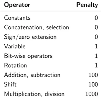
5.1 Operator penalties . . . 70
6.1 Solver failures by set . . . 93
7.1 MicroFormal test sets . . . 120
7.2 Fixed vs optimal reset strategy. Execution times in seconds 123 7.3 Performance of the MSPSAT algorithms . . . 126
7.4 Hit-rate of unsatisfiable core caching . . . 129
7.5 Performance on singleton sets when unsat core hits are re-moved . . . 130
7.6 Ample performance summary (execution times in seconds) 131 8.1 Performance on Max-SAT problems. . . 148
8.2 Performance on Pseudo-Boolean problems. . . 149
8.3 Performance on Max-SMT problems. . . 151
List of Figures
2.1 Bit-vector operations . . . 12
2.2 Bit-vector semantics . . . 14
2.3 Syntactic sugar . . . 15
2.4 MathSAT architecture overview . . . 18
4.1 Cases where propagation of unconstrained terms can occur 50 4.2 Core rewrite reduction . . . 52
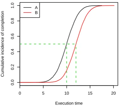
6.1 Example Cumulative Distribution Function plot . . . 78
6.2 Effect of techniques . . . 80
6.3 Pairwise interactions . . . 81
6.4 SAT versus DPLL(T) . . . 83
6.5 SAT versus DPLL(T) on real-world instances . . . 84
6.6 Effect of under-approximation on real-world instances . . . 85
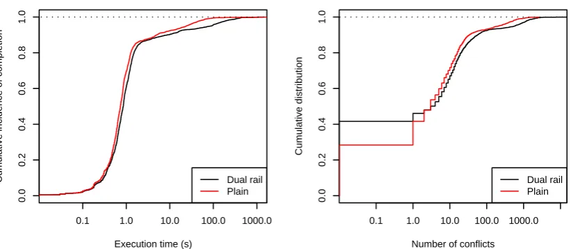
6.7 Effect of dual rail on real-world instances . . . 86
6.8 Effectiveness of rewriting in the core fragment . . . 87
6.9 Effect of packet splitting on simple processor instances . . . 88
6.10 Effect of difference propagation on lfsr instances . . . 89
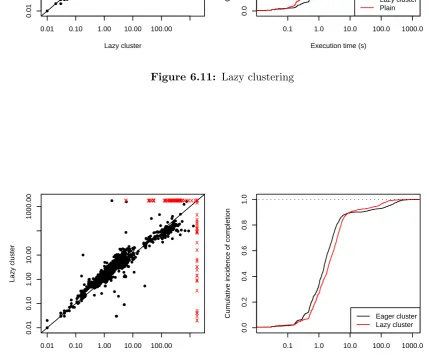
6.11 Lazy clustering . . . 90
6.12 Eager clustering . . . 90
6.13 CDF of comparison with other solvers . . . 92
6.14 CDFs of comparison with other solvers . . . 93
6.16 Overhead of model computation . . . 95
6.17 Model computation in Boolector . . . 98
6.18 Model computation in Z3 . . . 99
7.1 Intermediate representation language grammar . . . 105
7.2 Overview of the MicroFormal symbolic execution engine . 107 7.3 Cumulative frequency of set cardinality . . . 110
7.4 Pairwise formula similarity of instances . . . 112
7.5 Effect of reset interval on singleton calls . . . 121
7.6 Effect of reset interval on individual singleton calls . . . . 122
7.7 Effect of reusing solver information on SAGE instances. Ex-ecution times in seconds . . . 125
7.8 Effect of MSPSAT threshold on program 2 . . . 127
7.9 Effect of parallelism on a simple non-singleton set . . . 128
7.10 Ample execution performance . . . 132
Chapter 1
Introduction
Hardware and software systems have become incredibly complex and their usage is widespread. In designing these systems, verification is a highly challenging task. Hardware development costs are now routinely domi-nated by the verification effort, and there is a growing gap between our ability to design complex systems and the effort required to verify them, sometimes called the verification gap.
One avenue of research into closing this gap has been formal or semi-formal verification. A large number of techniques have been developed, including abstract interpretation, model checking, assertion based verifica-tion, equivalence checking, automatic test pattern generaverifica-tion, and many others. Many fully automated verification techniques depend on bit-precise reasoning to some extent, and this calls for the development of efficient and scalable techniques able to solve such formulae.
Chapter 1. Introduction
typically a vast array of different ways of encoding it into a corresponding SAT problem. Which encoding is chosen can have a very large impact on performance, and it may not be obvious which encoding is preferable without some knowledge of the inner workings of modern SAT solvers.
Solvers which reason at the level of bit-vectors can be seen as an answer to this problem. With these, the user can work at a higher level, not needing to worry about the low-level details of SAT solvers. Even if the bit-vector reasoner is implemented to ultimately use a SAT solver, the knowledge for how it is best used can be captured within the solver itself rather than in every application that needs to use it. A solver at the bit-vector level may also take advantage of the higher level of abstraction to either simplify the formula before attempting to solve it, or use alternative techniques in solving which may scale better for the formulae of interest to the user.
In recent years there has been an interest in solvers that support richer logics than propositional logic, and the field of Satisfiability Modulo Theo-ries (SMT) has risen as a response to this interest. SMT combines proposi-tional logic with one or more decidable theories such as linear arithmetic or bit-vectors to form a fully automated decision procedure at a higher level of abstraction. In the last few years, SMT has made tremendous progress, and SMT solvers are now being fielded in real-world applications both in academia and industry.
1.1. Contribution
1.1
Contribution
The contributions of this thesis lie in several novel techniques for solving of SMT formulae over the bit-vectors as well as some extensions to SMT. The main contributions can be summarised as follows:
– We introduce a simple and flexible framework for simplifying formu-lae based on term rewriting which is able to manage the potential complexity of simplification of bit-vector terms.
– We introduce several techniques, such as partitioning or variable split-ting, that enhances other well known preprocessing or solving tech-niques
– We show how models can be computed while still applying all prepro-cessing techniques, rather than resorting to disabling one or more of them when models are requested.
– We show how the major preprocessing techniques can be used in an incremental solver.
– We introduce some novel under- and over-approximation techniques for bit-vector formulae.
– We introduce a lazy clustering scheme for dividing the theory solver consistency checks into multiple independent partitions.
– We show how it is possible to use minimal model enumeration in the lazy schema of SMT solving.
– We demonstrate how reusing learnt information from solving previous formulae can deliver significant performance enhancements in a real-world application without added implementation complexity
– We provide an extensive experimental evaluation, giving insight into the efficiency of the various techniques.
Chapter 1. Introduction
representation of Pseudo-Boolean constraints without modification to the standard SMT solver architecture.
Apart from the contributions of this thesis, we also try to give an overview of some of the techniques implemented within our SMT solver MathSAT that are relevant for the theory of bit-vectors, in the hope that it may give some insight into the observed performance of the solver.
Rather than just present techniques which have been proven to work in practise, this thesis will also discuss some techniques whose value has not (yet) been proven, or seem to have limited applicability. Using experi-mental evaluation, we will attempt to conclude which technique provide a benefit, which have limited use, and which may be unhelpful.
1.2
Acknowledgements
The work presented here has been in part supported by Semiconductor Research Corporation (SRC) under Global Research Collaboration (GRC) Custom Research Project 2009-TJ-1880 “WOLFLING”.
1.3
Overview
The thesis is organised as follows. Preliminaries such as notation and basic concepts are introduced in chapter 2. Chapter3 describes techniques for solving formulae, chapter 4 covers techniques which simplify formulae before solving, and chapter 5 introduces approximation techniques.
1.3. Overview
Chapter 2
Preliminaries
Some background to the work presented in this thesis is necessary. In this chapter, we will introduce the concepts of propositional logic and the DPLL-style decision procedures often used to decide satisfiability in this logic. We will also introduce Satisfiability Modulo Theories, and how deci-sions procedures for this problem often works. Finally, we will give a brief overview of the MathSAT SMT solver, which is used as the proving ground for the techniques described in this thesis.
2.1
SAT
The satisfiability problem (SAT) is the problem of deciding satisfiability of formulae in propositional logic. Given a set of propositions B, a proposi-tional logic formula can be defined as
– ⊤ and ⊥ are formulae. – If p ∈ B, p is a formula
– If α and β are formulae, then ¬α and α∧β are formulae.
A truth assignment or interpretation µ is a mapping from propositions to truth values {false,true}. We will also see a truth assignment as a set
Chapter 2. Preliminaries
are mapped to false.
A truth assignment µ models the formula ϕ, denoted µ |= ϕ given by the following.
µ |= ⊤
µ ̸|= ⊤
µ |= p iff p∈ µ
µ |= ¬α iff µ̸|= α
µ |= α∧β iff µ|= α and µ|= β
The SAT problem can now be stated as the problem of determining for a given formula ϕ if there exists an interpretation such that µ |= ϕ. It is common to extend the language with several other connectives
– Disjunction ∨ defined as α∨β iff ¬(¬α∧ ¬β) – Implication ⇒ defined as α ⇒β iff (¬α)∨β
– Equivalence ⇔ defined as α ⇔ β iff α ⇒ β and β ⇒ α
We will call a truth assignment that gives values to all propositions in a formula ϕ a total truth assignment. A truth assignment which gives values to a strict subset of the propositions in a formula is called partial. We will define Atoms(ϕ) as the set of atoms in the formula ϕ.
Decision procedures for the SAT problem typically accept formulae in a particular form called Conjunctive Normal Form (CNF) defined as follows:
– An atom is a proposition p∈ B
– A literal is either an atom p or its negation ¬p. We say that a negated atom is a negative literal and a non-negated atom a positive literal. If l is a negative literal, by ¬l we mean the corresponding positive literal.
– A clause is a disjunction of literals, often seen as a set of literals. A clause containing a single literal will be called a unit clause.
2.2. Solving the SAT problem
All propositional formulae can be translated into CNF in linear time, if we are allowed to introduce fresh propositions as described in [Tse68]. Many variations on this technique have been proposed, and they may all be called Tseitin-style encodings meaning that they introduce fresh propositions to “give names” to subformulae allowing for a linear time translation.
2.2
Solving the SAT problem
The most popular approach to solving the SAT problem today is using a DPLL-style [DLL62] algorithm. In its most basic form, the algorithm may be outlined as in algorithm2.1taking a set of clauses as input and returning either ⊤ (the formula is satisfiable) or ⊥ (the formula is unsatisfiable).
Algorithm 2.1: Basic DPLL algorithm DPLL(ϕ)
if ϕ =∅ then 1
return ⊤ 2
end 3
if ∅ ∈ϕ then 4
return ⊥ 5
end 6
if Some {l} ∈ϕ then 7
return DPLL({c\ {¬l} |c∈ϕ∧l ̸∈c})
8
end 9
p←some atom in ϕ
10
return DPLL(ϕ∪ {p}})∨DPLL(ϕ∪ {¬p})
11
Chapter 2. Preliminaries
2.3
Satisfiability Modulo Theories
Satisfiability Modulo Theories (SMT) can be seen as an extension of propo-sitional logic with some theory of interest such as linear arithmetic. The following introduction to SMT follows standard lines, a good reference is [BHvMW09].
We let Σ = ⟨F,P⟩ be a signature containing a set of function symbolsF and a set of predicate symbolsP, each with an associated arity. We call the 0-arity function symbols constants, and the 0-arity predicates propositional symbols. We will call Fn the set of function symbols in F with arity n
and Pn the set of predicate symbols in P with arity n. In this thesis we will focus on the quantifier free formulae constructed using this signature, which we will call ground formulae. The (free) variables in formulae will be seen as uninterpreted constant symbols in Σ. Given a signature Σ = ⟨F,P⟩
formulae can be built according to the following
– If c ∈ F0 then c is a term
– If f ∈ Fn and t1, . . . , tn are terms, then f(t1, . . . , tn) is a term
– ⊥ and ⊤ are formulae
– If P ∈ P0 then P is a formula
– If P ∈ Pn and t1, . . . , tn are terms, then P(t1, . . . , tn) is a formula
– If α, β are formulae, then ¬α, α ∨ β, α ∧ β α ⇒ β and α ⇔ β are formulae
The concepts of atoms, literals, clauses, CNF, and unit clauses lifts from propositional logic in the natural way. We let Var(ϕ) be the set of variables in the formula ϕ and Atoms(ϕ) be the set of atoms.
2.4. Fixed-width bit-vectors
A Σ-structure is a tuple consisting of a universe, an assignment of vari-ables σ to elements in the domain, and an interpretation [[·]] of all other nonlogical symbols. A Σ-formula is a formula using nonlogical symbols in Σ. A sentence is a formula without variables. A theory is a set of Σ-sentences. Given a theory T, a Σ-formula is satisfiable iff there exists a Σ-structure that satisfies both the formula and all sentences of T. A Σ-formula is valid in T iff all Σ-structures that satisfy the sentences of T
also satisfies the formula.
The SMT-LIB1 provides a publicly available benchmarks library for SMT formulae in a number of different theories, as well as definitions of several theories of interest.
2.4
Fixed-width bit-vectors
We define a theory of fixed-width bit-vectors similar to the theory defined in the SMT-LIB, an overview of the operators can be found in figure 2.1. The operators in the SMT-LIB bit-vector theory which are not included here are still supported in MathSAT, but translated into the operators shown here rather than handled natively.
We define semantics for bit-vector atoms in a way similar to Brinkmann and Drechsler [BD02].
– A bit-vector constant x⟨n⟩ ∈ {0,1}n is a vector of n bits denoted (xn−1, . . . , x0).
– If x⟨n⟩ is a bit-vector, then x⟨n⟩[i] is the ith bit xi in x⟨n⟩.
– We define the auxiliary functions natn and bvn such that natn(x⟨n⟩) =
∑
i∈1...n2
nx(i−1) and we define bv
n to be the inverse of natn (bvn = nat−n1).
1Available at
Chapter 2. Preliminaries
t⟨1m⟩ ::t⟨2n⟩ Concatenation of two bit-vectors t⟨1m⟩ and t⟨2n⟩ t⟨n⟩[i:j] Selection of bitsj to i inclusively oft⟨n⟩
nott⟨n⟩ Bit-wise negation of all bits int
t1⟨n⟩andt2⟨n⟩ Bit-wise and of all bits int1 with all bits in t2 t1⟨n⟩ort2⟨n⟩ Bit-wise or of all bits int1 with all bits in t2 t1⟨n⟩≪t2⟨n⟩ Shift left of t1 by the amount given by t2
t⟨1n⟩≫lt⟨
n⟩
2 Logical shift right of t1 by the amount given by t2
t⟨1n⟩≫at⟨
n⟩
2 Arithmetic shift right of t1 by the amount given by t2 t⟨1n⟩rolc Rotate left oft1 by the amount given byc∈[0, n−1] t⟨1n⟩rorc Rotate right of t1 by the amount given by c∈[0, n−1]
zext⟨m⟩(t⟨n⟩) Zero extension oft to a bit-vector of m bits (m≥n)
sext⟨m⟩(t⟨n⟩) Sign extension oft to a bit-vector of m bits (m≥n) t1⟨n⟩+t2⟨n⟩ Addition oft1 and t2
t1⟨n⟩−t2⟨n⟩ Subtraction oft1 and t2 −t⟨n⟩ Unary subtraction
t1⟨n⟩∗t2⟨n⟩ Multiplication oft1 and t2
t⟨1n⟩/ut⟨
n⟩
2 Unsigned division betweent1 and t2
t⟨1n⟩/st⟨
n⟩
2 Signed division betweent1 and t2
t⟨1n⟩remut⟨
n⟩
2 Unsigned remainder
t⟨1n⟩remst⟨
n⟩
2 Signed remainder
t⟨1n⟩<ut⟨
n⟩
2 Unsigned less than
t⟨1n⟩<st⟨
n⟩
2 Signed less than
t⟨1n⟩≤ut⟨
n⟩
2 Unsigned less than or equal
t⟨1n⟩≤st⟨
n⟩
2 Signed less than or equal
2.5. Approaches to SMT
– We define + as addition, · as multiplication, /as division over natural numbers.
– We let σ be an assignment of variables to values in their domain, and define [[t]]σ as the interpretation of the bit-vector term or atom t.
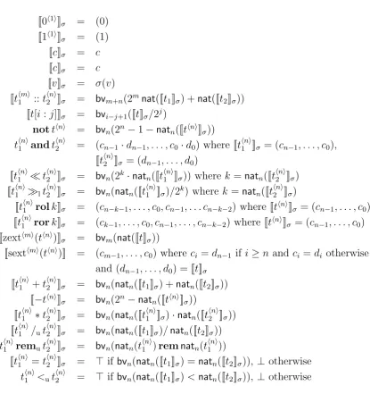
The semantics for most of the bit-vector operators can be seen in figure
2.2, and the rest are defined in terms of other operators in figure 2.3. When the specific width of a bit-vector term t⟨n⟩ is either irrelevant or clear from the context, it will often be dropped and we will simply write t.
2.5
Approaches to SMT
There are several different approaches to solving SMT formulae, they can be divided into two main categories of techniques called the eager and the lazy approaches.
2.5.1 Eager encoding into SAT
In the eager encoding into SAT the formula is translated into an equisatis-fiable SAT instance which can then be solved in any SAT solver. How this translation is performed is theory-specific, for the theory of bit-vectors it can be performed by a process calledbit-blasting or flattening which is ba-sically the same technique used in hardware sysnthesis to generate a netlist from combinational RTL.
2.5.2 Lazy encoding
Chapter 2. Preliminaries
[[0⟨1⟩]]
σ = (0)
[[1⟨1⟩]]
σ = (1)
[[c]]σ = c
[[c]]σ = c
[[v]]σ = σ(v)
[[t⟨1m⟩ ::t⟨2n⟩]]σ = bvm+n(2mnat([[t1]]σ) +nat([[t2]]σ))
[[t[i:j]]]σ = bvi−j+1([[t]]σ/2j)
nott⟨n⟩ = bv
n(2n−1−natn([[t⟨n⟩]]σ))
t⟨1n⟩andt⟨2n⟩ = (cn−1·dn−1, . . . , c0·d0) where [[t⟨
n⟩
1 ]]σ = (cn−1, . . . , c0),
[[t⟨2n⟩]]σ = (dn−1, . . . , d0)
[[t⟨1n⟩≪t⟨2n⟩]]σ = bvn(2k·natn([[t⟨ n⟩
1 ]]σ)) where k =natn([[t⟨ n⟩
2 ]]σ)
[[t⟨1n⟩≫lt⟨ n⟩
2 ]]σ = bvn(natn([[t⟨
n⟩
1 ]]σ)/2k) where k=natn([[t⟨ n⟩
2 ]]σ)
[[t⟨1n⟩rolk]]σ = (cn−k−1, . . . , c0, cn−1, . . . cn−k−2) where [[t⟨n⟩]]σ = (cn−1, . . . , c0)
[[t⟨1n⟩rork]]σ = (ck−1, . . . , c0, cn−1, . . . , cn−k−2) where [[t⟨n⟩]]σ = (cn−1, . . . , c0)
[[zext⟨m⟩(t⟨n⟩)]]
σ = bvm(nat([[t]]σ))
[[sext⟨m⟩(t⟨n⟩)]] = (c
m−1, . . . , c0) whereci =dn−1 if i≥n and ci =di otherwise
and (dn−1, . . . , d0) = [[t]]σ
[[t⟨1n⟩+t2⟨n⟩]]σ = bvn(natn([[t1]]σ) +natn([[t2]]σ))
[[−t⟨n⟩]]
σ = bvn(2n−natn([[t⟨n⟩]]σ))
[[t⟨1n⟩∗t2⟨n⟩]]σ = bvn(natn([[t⟨ n⟩
1 ]]σ)·natn([[t⟨
n⟩
2 ]]σ))
[[t⟨1n⟩/ut⟨ n⟩
2 ]]σ = bvn(natn([[t1]]σ)/natn([[t2]]σ))
[[t⟨1n⟩remut⟨ n⟩
2 ]]σ = bvn(natn(t⟨
n⟩
1 )remnatn(t⟨
n⟩
1 ))
[[t⟨1n⟩ =t2⟨n⟩]]σ = ⊤ if bvn(natn([[t1]]σ) =natn([[t2]]σ)),⊥ otherwise
t⟨1n⟩<ut⟨
n⟩
2 = ⊤ if bvn(natn([[t1]]σ)<natn([[t2]]σ)),⊥ otherwise
2.5. Approaches to SMT
t⟨1n⟩ort⟨2n⟩ = not((nott⟨1n⟩)and(nott⟨2n⟩))
t⟨1n⟩≫at⟨
n⟩
2 = ite(t
⟨n⟩
1 [n−1] = 0⟨1⟩, t
⟨n⟩
1 ≫lt⟨
n⟩
2 ,not((nott
⟨n⟩
1 )≫at⟨
n⟩
2 ))
t⟨1n⟩−t⟨2n⟩ = t⟨1n⟩+ (−t⟨2n⟩)
t⟨1n⟩/st⟨
n⟩
2 = ite(t
⟨n⟩
1 ≤s0∧t⟨
n⟩
2 ≤s0, t⟨
n⟩
1 /ut⟨
n⟩
2 ,not(u1/uu2)) where u1 = ite(t⟨
n⟩
1 <s0,nott⟨
n⟩
1 , t
⟨n⟩
1 ) and u2 = ite(t⟨ n⟩
2 <s0,nott⟨
n⟩
2 , t
⟨n⟩
2 )
t⟨1n⟩remst⟨
n⟩
2 = ite(t
⟨n⟩
1 ≤s0∧t⟨
n⟩
2 ≤s0, t⟨
n⟩
1 remut⟨
n⟩
2 ,not(u1remuu2)) where u1 = ite(t⟨
n⟩
1 <s0,nott⟨
n⟩
1 , t
⟨n⟩
1 ) and u2 = ite(t⟨ n⟩
2 <s0,nott⟨
n⟩
2 , t
⟨n⟩
2 )
t⟨1n⟩≤ut⟨
n⟩
2 = ¬(t
⟨n⟩
2 <ut⟨
n⟩
1 )
t⟨1n⟩≤st⟨
n⟩
2 = ¬(t
⟨n⟩
2 <st⟨
n⟩
1 )
t⟨1n⟩<st⟨
n⟩
2 = ite(t
⟨n⟩
1 [n−1] = t
⟨n⟩
2 [n−1], t
⟨n⟩
1 <ut⟨
n⟩
2 , t
⟨n⟩
1 = 1⟨n⟩)
Figure 2.3: Syntactic sugar
atoms. We call the logical structure of the formula the propositional ab-straction [Pla81] of the formula.
Definition The propositional abstraction of a ground formula ϕ is a propo-sitional formula where all predicates in ϕ are replaced with propositions.
The lazy approach to SMT divides the reasoning into two parts; reason-ing on the propositional abstraction of the formula, and reasonreason-ing in the theories of the formula. For the propositional abstraction a boolean enu-merator is used, typically implemented using a DPLL-style SAT solver. The SAT solver proceeds by assigning truth values to atoms in the propo-sitional abstraction, keeping track of the current truth assignment.
The SAT solver communicates the current truth assignments to the theory solvers, which given a set of such truth assignments determines consistency of the assignment in the theory. In the theory solver, this truth assignment is seen as a set of literals L1, . . . , Ln which are positive
Chapter 2. Preliminaries
set of literals, or the last extension of the truth assignment can be retracted. Further, when the theory solvers determine that the current truth as-signment is inconsistent in the theory, a conflict set is produced which encapsulates the reason for the inconsistency. The conflict set is a subset of the current truth assignment, which in itself is inconsistent in the the-ory. This conflict set is used by the SAT solver to produce a conflict clause, which is used to prune further search.
Theory solvers are also allowed to deduce truth assignments to currently unassigned theory atoms. A deduced truth assignment is one which is a logical consequence in the theory of the current truth assignment, and will help the SAT solver prune the search.
Several improvements to the basic lazy approach have been proposed, see [Seb07, BHvMW09] for an overview.
2.6
DAG representation of formulae
It has become a staple in SMT solvers to represent formulae using perfect sharing, sometimes also called aggressive sharing, structural hashing, hash consing, or common subexpression elimination. The plethora of names may be due to its popularity in many different fields such as functional programming languages [Got76], theorem proving [RV01] and compiler op-timisation [Coc70]. Instead of storing a formula as a tree, it is stored as a directed acyclic graph (DAG). A subformula or term which is used sev-eral times in the formula will be represented with a single node in this DAG. Because formulae are represented in this way, we will use this when considering the number of occurrences of subformula or terms in a given formula.
2.7. MathSAT
incoming edges.
Example 2.1
Take the formula x+ 1<u(x+ 1)∗2. The DAG representation of this term is
shown below
<u
∗
+ 2
x 1
and we can see that x + 1 occurs twice in this formula, while the variable x
only occurs once.
2.7
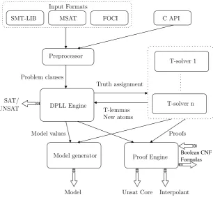
MathSAT
MathSAT [BCF+08] is a SMT solver following the lazy schema, an overview of the architecture can be seen in 2.4. It accepts input in a number of different input formats, and also provides an API allowing MathSAT to be linked into other applications.
Chapter 2. Preliminaries
Boolean CNF Formulas
T-solver n T-solver 1
DPLL Engine
Truth assignment
Model generator
Model
FOCI
MSAT C API
Interpolant Problem clauses
SMT-LIB
SAT/ UNSAT
Preprocessor Input Formats
Unsat Core Proof Engine
Proofs Model values
T-lemmas New atoms
Figure 2.4: MathSAT architecture overview
2.7.1 Preprocessing
The preprocessor consists of several different parts: Simplification, conver-sion to CNF, static learning and initialisation of the solver.
Simplification During simplification the goal is to produce a new simpler
formula which is equisatisfiable to the original. It is also required that given any model for the simpler formula it is possible to compute a model for the original formula. Examples of simplifications are computing a canonical form for atoms in linear arithmetic.
CNF conversion Conversion into CNF is performed with a Tseitin-style
2.7. MathSAT
Static learning Static learning will add some lemmas for the atoms
occur-ring the formula. These lemmas are clauses which may help prune search, an example is lemmas for transitivity.
Solver initialisation Lastly the CNF is fed to the solver, and the solver
is initialised. In this step the preprocessor instructs the solver to allocate the appropriate theory solvers and also provide some heuristic information about the formula which may help improve performance.
2.7.2 The solver proper
The heart of the solver is a boolean enumerator based on the MiniSat DPLL-style SAT solver, which enumerates models of the propositional ab-straction of the formula. These models correspond to a truth assignment to the theory atoms, and this truth assignment is communicated to the theory solvers. The theory solvers receives these, and determines if this truth assignment is consistent in the theory.
2.7.3 Theories
MathSAT supports many of the theories of interest in practical applica-tions, namely
– Equality and uninterpreted functions (EUF) – Extensional arrays (ARR)
– Difference logic (DL)
– Unit two variable per inequality (UTVPI).
Chapter 2. Preliminaries
2.7.4 API
The MathSAT API is similar to that of Yices or Z3. The relevant opera-tions are
Assert ϕ Assert that a formula must be true
Push backtrack point Remember the current state
Pop backtrack point Restore the state at the last backtrack point Solve Solve the conjunction of assertions in the current state
In order to solve the three formulae α, α ∧β and α∧ γ we can do this in the following way
1. Assert α
2. Solve
3. Push backtrack point 4. Assert β
5. Solve
6. Pop backtrack point 7. Assert γ
8. Solve
When backtracking to a previous state, the solver is free to retain in-formation which has been learnt previously which may help solve future formulae. An example is the theory conflicts which are universally valid and can therefore be reused regardless of what future formulae may look like.
2.7.5 Performance
Since the start of the annual SMT competition2 MathSAT has been taking part in all categories it can support. The results are in brief:
2SMT-COMP is available at
2.7. MathSAT
– In 2005, MathSAT competed in 6 categories, placing second in one and third in 5.
– In 2006, MathSAT competed in 8 categories, placing second in two and third in 4.
– In 2007, MathSAT competed in 7 categories, placing second in two and third in two.
– In 2008, MathSAT competed in 9 categories, placing second in 3 and third in 4.
– In 2009, MathSAT competed in 12 categories, placing first in the bit-vector category and the category combining uninterpreted functions and integer difference logic. It also placed second in 7 categories and third in one.
2.7.6 Further reading
Chapter 3
Solving techniques
There are two main techniques for solving bit-vector formulae that are used within MathSAT: Translation into SAT and the lazy approach to SMT, also called DPLL(T). Both the eager encoding into SAT and the lazy approach are in this work based on bit-blasting to handle bit-vector atoms. In this chapter, we will look at how these two techniques are used within MathSAT, as well as some auxiliary techniques such as layering, static learning, or modifications to the basic boolean enumeration algorithm.
We will start this chapter by looking at bit-blasting, since it is used in both approaches to solving. Then we will discuss the lazy approach and give some details on the bit-vector theory solver, followed by the eager approach. We continue with the use of EUF layering in MathSAT, static learning, clustering, and minimal model enumeration.
3.1
Bit-blasting
Chapter 3. Solving techniques
CNF turned out to be unnecessarily slow on large but trivial instances. A disadvantage of going directly to CNF is that propositional preprocessing techniques such as those described in [BB06] can not be applied.
Each atom is converted using a Tseitin-style CNF transformation [Tse68], taking care that each atom is represented by a propositional literal, which is not added (as a unit) to the CNF but kept separate. In this way, the CNF for a particular literal is guaranteed to be satisfiable. Adding the representative literal asserts that the atom is true and adding the negation of the literal asserts that the atoms is false. Example 3.1 shows how this might work in practise.
Example 3.1
We can bit-blast and convert the atom x⟨1⟩<uy⟨1⟩ into CNF by adding one
fresh Tseitin variable v which is meant to “represent” the atom and create the
clauses
{¬v,¬x}, {¬v, y}, {v, x,¬y}
If in the truth assignment the atom is true, we solve these clauses under the
assumption of v. It the atom is false, we solve under the assumption ¬v.
Most bit-vector terms are bit-blasted in a straightforward way. E.g. relations are bit-blasted using comparators, addition and subtraction using ripple-carry adders and so on. Some small concessions to performance have been done, such as strength reduction for multiplication or division by constant [War02].
3.2
DPLL(T) or the lazy schema
3.2. DPLL(T) or the lazy schema
Incrementality The current truth assignment is extended incrementally by communicating the new truth assignments to the theory solver. Backtrackability During backtracking, a number of the literals on the
truth assignment are retracted. The retracted literals are always those last added
Consistency checking Given a particular truth assignment, the theory solver should be able to detect inconsistent truth assignments, and be able to provide models for consistent truth assignments.
Conflict set generation For inconsistent sets of literals a conflict set should be communicated back to the boolean enumerator. This is a subset of the current truth assignment, which in itself is inconsistent.
The underlying SAT solver is a modified version of MiniSat [ES04], with the following modifications
– Component caching [PD07b], sometimes also called progress saving or phase caching. This is a technique which stores the phase of all assignments made, and when making a new decision it checks the last decision made on this variable and makes the same one.
– Blocking literals [SE08]. This helps reduce the number of memory references for unit-propagation on already satisfied clauses. A copy of one of the literals is kept in the watch list data structure. If this literal is satisfied, there is no need to visit the clause itself.
– More frequent restarts than the restart strategy implemented in Min-iSat.
Chapter 3. Solving techniques
SAT solver; In this way, the CNF for each atom is guaranteed to be satisfi-able. In order to check consistency of a set of bit-vector literals, L1, . . . , Ln
we collect the corresponding Tseitin literals l1, . . . , ln, negating them iff the
bit-vector literal was negative. We then solve the bit-blasted formula as-suming this set of literals enforcing the truth values of the atoms. Solving under assumption of a number of literals is supported in a number of SAT solvers, like MiniSat [ES04] or PicoSAT [Bie08].
Should the formula be unsatisfiable under these assumption, we can compute a conflict in terms of the assumed literals. This can be used to compute a conflict set, which although not guaranteed to be minimal, often is minimal or close to minimal in practise.
There are also a number of other features of theory solvers, which al-though not strictly necessary may be advantageous:
Early pruning Checking consistency of partial truth assignments Deduction Deducing literals not currently on the truth assignment For early pruning, we will use what we shall call bounded SAT reasoning.
3.2.1 Bounded SAT reasoning
3.3. Eager encoding to SAT
3.2.2 Deduction
It is also possible to deduce literals. A simple way is to perform unit propagation, and then deduce all literals which have been given a truth value by the unit propagation. However this is not yet implemented in MathSAT.
3.3
Eager encoding to SAT
The eager approach to SMT consists of solving formulae by translation into an equisatisfiable SAT problem, and solving that in a standard SAT solver. For bit-vectors this translation is straightforward, by what is called bit-blasting or flattening.
3.3.1 Implementation issues
To achieve this encoding in a DPLL(T) style solver like MathSAT without major modification, there are two different approaches:
– Bit-blast the formula in preprocessing. This will produce a purely propositional formula, which can be solved by the boolean enumerator without the help of any theory solver.
– Convert the formula into a bit-vector atom. Propositions can be re-placed with fresh single-bit bit-vector variables, and the logical struc-ture of the formula can be encoded using bit-wise operators. This atom can then be solved by the bit-vector theory solver.
Chapter 3. Solving techniques
a conjunction of bit-vector atoms. The implicit transformation is simply implemented by marking all conjuncts as bit-vector atoms. The boolean enumerator will then treat these as if they were real bit-vector atoms, and the theory solver is extended with support for bit-blasting bit-vector for-mulae instead of just atoms.
3.4
Theory solver layering
A technique which has been in use for some time in MathSAT is layering [BBC+05b]. The underlying idea is that given a truth assignment that is unsatisfiable it is frequently very “obviously” inconsistent. Reasonably it should therefore be correspondingly easy to detect the inconsistency, and there should be no need to use a potentially expensive decision procedure to do so. In MathSAT, it is possible to allocate a number of different the-ory solvers which will each handle some subset of the atoms in the formula or reason on an abstraction of the atoms. As an example, for linear arith-metic, one can allocate one EUF solver treating all arithmetic operators as uninterpreted functions, one difference logic solver only considering the subset of atoms in difference logic, and finally a theory solver for full lin-ear arithmetic, which can be used when all else fails. For bit-vectors, it is possible, apart from using a solver for bit-vectors, to also use a solver for EUF as a layer above the bit-vector solver. The intuition is that in cases when it can aid in search it will do so at low cost, and in cases where it cannot it is a very low overhead compared to a full bit-vector solver.
3.5. Static learning
This gives the EUF some extra capability of detecting conflicts over bit-vectors while still maintaining the same computational complexity and efficiency.
3.5
Static learning
The idea behind static learning [BBC+05b, YM06] is to add lemmas which are valid in the theory. This is done by instantiating a few basic axioms, such as axioms for transitivity of equality, mutual exclusion of inequality and similar.
3.6
Clustering
The idea of dividing the set of theory atoms into independent sets, called clustering was first introduced in [BBC+05a] for EUF and linear arithmetic, but it generalises also to other theories. Before search starts, the theory atoms are divided into a set of independent sets each of which can not interfere with the satisfiability of any other. Then for each such set, a separate theory solver is used. In this way we can reduce the amount of theory literals each theory solvers need to reason with, and hopefully avoid some unnecessary complexity.
Definition Two atoms A1, A2 belong to the same cluster iff Var(A1) ∩
Var(A2) ̸= ∅
Definition A clustering of a set of atoms A is a partition of this set induced by the cluster relation.
Chapter 3. Solving techniques
truth assignment of literals when using the lazy schema. The former has been applied in MathSAT in the past [BBC+05b], and applied for the the-ory of bit-vectors in [BCF+07]. For the industrial bit-vector instances used in the latter paper, the clustering typically generated hundreds of clusters, so it would appear to be very efficient. Looking closer however, most of these clusters contain a handful of atoms containing a single variable, mak-ing these clusters trivial. There was also often one large cluster containmak-ing most of the atoms. Most of the complexity of reasoning remains in this large cluster.
To achieve a more fine-grained clustering, a local rather than global ap-proach must be taken, and if we are using the lazy schema this is possible to do. Instead of clustering all theory atoms up-front during preprocess-ing, we can attempt to cluster all literals occurring on each truth assign-ment. Since this may be a subset of all atoms, there is the possibility that this will produce more clusters, and simpler problems to solve. For every truth assignment of literals L, we perform clustering of the set of atoms Atoms(L) on that truth assignment producing several clusters of literals L1, L2, . . . , Ln. Each cluster can now be checked for consistency
independently.
Clustering of truth assignments makes it more difficult to build a theory solver which retains information from one consistency check to the next however, because the clusters of literals may be different from one call to the next. We can still create an incremental theory solver that retains learnt information, if we relax the requirement for clustering a little.
3.7. Minimal model enumeration
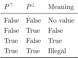
Table 3.1: Three value logic semantic of dual rail encoding
P⊤ P⊥ Meaning False False No value False True False True False True True True Illegal
in more than one cluster currently created, these clusters are merged into a single cluster. This is done by identifying the largest of these clusters and merging all others into it. The other clusters are then removed and the new atom added to the merged cluster. This is just an approximation of the original clustering technique because for a given truth assignment, some clusters on that truth assignment may now be handled by a single theory solver.
3.7
Minimal model enumeration
We would like to reduce the number of literals sent to the bit-vector theory solver, since each theory solver call is potentially very expensive. One way to do this is to have the boolean enumerator enumerate minimal models. In [RC06], Roorda and Claessen uses a technique based on a dual-rail encoding which gives minimal models for the SAT problem, and the same technique lifts into SMT.
Chapter 3. Solving techniques
3.7.1 Sign-Minimal Models
To see why this encoding would help in enumerating minimal models, we can notice that in DPLL, if the decision heuristic always assigns false to decision variables, then any model µ for a set of clauses Γ has the minimal number of positive literals. This means that it is not possible to negate any of the positive literals in µ and still have µ|= Γ. We say that such a model is (positive) sign-minimal. The reverse is true if the decision heuristic always assigns true to decision variables, and we call such models negative sign-minimal.
To prove this, we show an invariant that holds during search. We show that there exists a subset of Γ such that the current interpretation µ will always be a sign-minimal model for that subset. Let us call Σ ⊆ Γ the interesting subset. We will only cover the case were the heuristic assign false, the other case is analogous.
Init We have that µ = ∅. Let Σ = ∅, and µ will be a sign-minimal model
of Σ.
Decision Making a decision on a variablev will add¬v toµ. The extended interpretation will still be a sign-minimal model of Σ.
Unit Propagation If a literal l is unit-propagated, the reason is a clause
in Γ \Σ, since it has to be an unsatisfied clause, and all clauses in Σ are satisfied under µ. If we extend Σ with this new clause, the extended µ will be a sign-minimal model of the extended Σ.
Backtracking If we backtrack to a previous decision level, we can remove
3.7. Minimal model enumeration
decision level. Therefore, the reduced µ will be a sign-minimal model for the reduced Σ.
Adding a Conflict Clause For any new conflict clause c, Γ |= c. So, for any
µ′, µ′ |= Γ iffµ′ |= Γ∪{c}. Therefore, an interpretation µ′ is a sign-minimal model of Γ iff it is also a sign-minimal model of Γ∪ {c}.
Complete models In a complete model, the invariant gives us that µ is a
sign-minimal model for a subset of the clauses. Therefore, it must also be a sign-minimal model for all clauses.
3.7.2 Minimality for Standard Dual Rail
Sign-minimality and assigning decision variables to false gives us minimal-ity in dual rail, since only assignments to true on dual rail atoms correspond to an assignment in the three value logic.
3.7.3 Minimality in SMT
In MathSAT, all theory conflicts consist of all negative dual rail literals. They can never in themselves force a truth value to any literal, and so minimality for the propositional abstraction is preserved.
For theory deduction, it can be encoded as an implication clause which is identical to the conflict clause that would have been added had the implied literal been assigned the inconsistent truth value. Therefore minimality is preserved.
3.7.4 Encoding of non-CNF formulae
Encoding of non-CNF formulae is straightforward. For every subformulaϕ
Chapter 3. Solving techniques
Table 3.2: Dual-rail encoding of connectives
Connective Encoding
α∧β ⟨α⊤∧β⊤, α⊥∨β⊥⟩
α∨β ⟨α⊤∨β⊤, α⊥∧β⊥⟩
¬α ⟨α⊥, α⊤⟩
dual rail encoding would be simply ⟨α⊤ ∧β⊤, α⊥∨ β⊥⟩. An encoding for some common connectives can be seen if figure 3.2. Translation to CNF can be performed in the normal way of the two formulae in the tuple.
3.7.5 Redundancy
The minimal model enumeration shown here does come with a price, and the price to pay is in redundancy [ABC+02] of enumerated models.
Definition Given a set of interpretations I = {µ1, µ2, . . . , µN}, we say
that this set is non-redundant iff for every µi ∈ I the set I′ = I \ {µi} is
not a cover of I.
3.7. Minimal model enumeration
Example 3.2
Take the formula (A ∧B) ∨ (¬A ∧C) ∨ (¬B ∧ ¬C). This formula has the
following minimal models
{A, B}
{¬A, C}
{¬B,¬C}
{¬A,¬B}
{B, C}
{A,¬C}
In this example, it is enough to enumerate either the first three or the last three
to cover all models of the formula. However, with a dual-rail encoding we will
enumerate all six. This is easy to see by stepping through enumeration. The
formula can be written in CNF as {A,¬B, C}, {¬A, B,¬C}, and encoded in
dual rail the formula becomes
{A⊤, B⊥, C⊤}, {A⊥, B⊤, C⊥}
plus the clauses ruling out the forbidden value for each original variable, not
show here. One model for this is{A⊤,¬A⊥, B⊤,¬B⊥,¬C⊤¬C⊤}
correspond-ing to the minimal model{A, B}. Adding a blocking clause{¬A⊤,¬B⊤}. We
can iterate until we have found the next two models, adding the corresponding
blocking clauses
{¬A⊤,¬B⊤}, {¬A⊥,¬C⊤}, {¬B⊥,¬C⊥}
Even though we have now covered all models, the set of clauses are still
sat-isfied, e.g. with the model
Chapter 3. Solving techniques
and it is only when blocking clauses for all minimal models have been added
Chapter 4
Preprocessing
Many instances, especially those coming from practical application of de-cision procedures in industry have an inefficient encoding. There may be a great number of redundancies, subformulae which are trivially unsatis-fiable, and irrelevant subformulae which do not affect satisfiability. These may cause significant slowdown when trying to solve a formula when com-pared to a more clever encoding of the same problem.
In this chapter, we will look at some preprocessing techniques which can help in producing a simpler equisatisfiable formula from the input instance which can be fed into the underlying solver. The requirements for all preprocessing is
1. The preprocessed formula must be equisatisfiable to the original 2. For any model of the preprocessed formula, it must be possible to
compute a model for the original formula.
Chapter 4. Preprocessing
support this.
In this chapter we will look at a number of different techniques:
Normalisation Basic simplifications
Substitution Eliminating variables or propositions
Propagation of unconstrained terms Removing irrelevant parts of the formula
Disjunctive partitioning Splitting the formula into independent parts Packet splitting Splitting variables into several parts
Difference propagation Taking advantage of the fact that we know terms to be different from one another
Miscellaneous A collection of minor techniques
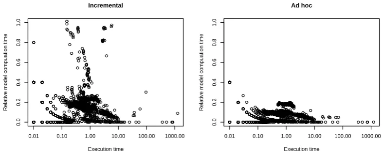
We will also see how model can be efficiently computed while using all the above techniques, how we can support preprocessing techniques in an incre-mental solver, and a few words on the architecture used for preprocessing in MathSAT.
4.1
Normal form computation
In formulae generated in real-world applications, the encoding of the prob-lem is often filled with terms which can be trivially simplified. Let’s look at a small motivational example:
Example 4.1
Given the equality x+ 2−(y −1) = 2∗x+ 3 which we would like to solve,
we can see several opportunities for simplification. We can start by simplifying
the left hand side into x−y+ 3 = 2∗x+ 3and then into y = 2∗x−x+ 3−3
which further simplifies into y = x.
4.1. Normal form computation
canonical form for bit-vector atoms. This is however an expensive propo-sition, it is in fact NP-hard [BDL98]. A more appealing alternative is to perform simplifications which although not producing a canonical form are both effective in practise and induces a low computational overhead. There are many ways of implementing simplifications such as those seen in exam-ple 4.1. In this thesis we will see simplifications as rewrite rules forming a simple term rewrite system.
Definition A rewrite rule, written s → t, has the property that s is not a variable and Var(t) ⊆ Var(s). A term rewriting system (TRS) is a set of rewrite rules.
Example 4.2
A simple rewrite rule for addition is 0 +x → x
Rewrite rules are unless explicitly specified defined on non-fixed size bit-vectors, the above example can be used to simplify addition with zero for all bit-vector widths, it could also be written as 0⟨n⟩ + x⟨n⟩ → x⟨n⟩ An example of a rule for a specific width might be
1⟨1⟩+ x⟨1⟩ → not(x)
which is applicable only on bit-vectors of width 1. Simplification is done by applying all rewrite rules to a fix-point, in term rewriting called the reflexive transitive closure, denoted t →∗ t′. Given a term rewriting sys-tem, a term which cannot be rewritten any further is said to be in normal form, and hence we will call these basic simplifications of bit-vector terms normalisation. For more information on term rewriting, Baader and Nip-kow [BN98] is a good introduction. Here we will introduce only the parts necessary in this application.
A rewrite rule s → t is applicable on a term u iff the left hand side t
Chapter 4. Preprocessing
Definition Given two terms s and t, the matching problem is the problem of deciding whether there exists a substitution σ such that σ(s) = t.
For instance the rewrite rule in example 4.2 is applicable on the term
0⟨32⟩+ (y⟨16⟩ :: z⟨16⟩)
with the substitution σ = [x 7→ y⟨16⟩ :: z⟨16⟩]. In this work we will use conditional rewrite rules. A conditional rewrite rules is of the form
s, c1, . . . , cn → where c1, . . . , cn are conditions which must all be fulfilled
for the rule to be applicable. An example of a conditional rewrite rule is
x⟨n⟩[u : l], u = n−1, l = 0 →x⟨n⟩ which removes “unnecessary” selection operators. We also define some predicates and functions which can be used in conditions, such as
– const(t), which is true iff t is a bit-vector constant
– nat(t), which converts t to the corresponding natural number if it is a constant
– eval(t), which given a bit-vector term not containing any variables, evaluates it to the corresponding bit-vector constant.
– t1 ≺ t2, a total ordering on terms – =, which check if two terms are equal
– The logical connectives ¬, ∨ with the usual meaning
The eval function can also be used in the right hand side of rules. Using these operators, it is possible to define rules likex+y, const(x), const(y) →
eval(x + y) for evaluation of additions, or x + y, y ≺ x → y + x which encodes commutativity of addition as a rewrite rule.
An important property for rewrite systems is termination, which is de-fined as follows.
4.1. Normal form computation
There are two ways of causing non-termination for bit-vector rewrites.
– We may have cyclic rewrites such that t1 → t2 → . . . → tn → t1, e.g.
the rewrite rule x+y → y +x.
– We may have a rewrite system which can grow the size of a term indefinitely. E.g., the rule x → x+ 0.
In general, given a term and a rewrite system, there may be several rules in the rewrite system which are applicable at the same time. A rewrite system that will always produce the same result regardless of the order of rule applications is called confluent.
Definition A rewrite system R is confluent iff for all s, t, t′, whenever
s→∗ t and s→∗ t′ there exists a u such that t →∗ u and t′ ∗→u.
In our case we do not require confluence. Instead rules are applied in the order in which they are declared, which means that the rewrite system does not need to be confluent, or even terminating with an arbitrary rule application order. This means that for every rule, it is possible to take advantage of the fact that we can assume that none of the previous rules could be applied. As an example of how this can be used, take the following two rules which evaluate addition over constants, and reorders addition with constant and some other term:
t1 +t2, const(t1), const(t2) → eval(t1 +t2)
t1 +t2, const(t2) → t2 +t1
This rewrite system is clearly not terminating, since for a term 1 + 2 the second rule could be applied infinitely many times. To achieve termination with an arbitrary rule application order, the second rule would have to be written as
Chapter 4. Preprocessing
Example 4.3
If we define the following simple term rewrite system for additions
0 +t → t
t1 +t2, ¬const(t1), const(t2) → t2 +t1
t1 + (t2 +t3), ¬const(t1), const(t2) → t2 + (t1 +t3)
Using this TRS we can rewrite the term x+ (y+ 2) by performing the following
rewrites x+ (y+ 2) → x+ (2 +y) →2 + (x+y).
4.1.1 A simple rule language
In MathSAT, close to 300 rewrite rules have been defined. Implementing all these rules by hand can be a time-consuming and error prone process, and therefore a simple rule language have been developed which allows for easy definition of new rules, and reduces the risk of introducing errors. Two simple examples of rewrites for trivially unsatisfiable or valid atoms are the following
bvult(t, t) ---> false;
bvule(t, t) ---> true;
The language supports all bit-vector operators supported by MathSAT and the rewrite rule predicates and operators discussed earlier, and the bit-vector operators are named similarly to the names used in the SMT-LIB. There is also some syntactic sugar meant to make the writing of rules easier. As an example, identifiers starting with c are interpreted as constants. So the rule
4.1. Normal form computation
would be equivalent to the rule
bvadd(t1, t2), const(t2) ---> bvadd(t2, t1);
To achieve reasonable performance, memoization is used to cache the result of previous rule applications. In addition, some basic filtering on rules are done before checking whether they can be applied to a given term.
Currently, this normalisation language is not available to users. Instead, it is translated into C++ code at compile time and linked into MathSAT. It may be that some interesting rules can not be expressed in the nor-malisation language in its current form. In these cases, they can be written by hand and added to the normalisation engine in the same way as gener-ated rules. Another option would be to extend the rule language to support the necessary features. Since rules are generated at compile time, there is not yet any reason to have a rule language that supports any possible rule that may be interesting, and the choice between extending the language or implementing new rules which cannot be expressed in the rule language by hand becomes a pragmatic one.
4.1.2 Rule verification
It is easy to introduce erroneous normalisation rules for bit-vector arith-metic, mostly because of a natural tendency to think in terms of standard arithmetic over the integers. Take for instance the following simple exam-ple
Example 4.4
The rule
t1 +t2<ut3, const(t2), const(t3) →t1<ut3 −t2
would be correct in ordinary linear arithmetic, but not in bit-vector arithmetic.
Chapter 4. Preprocessing
using the rule into v⟨8⟩<u3⟨8⟩ (assuming an additional rule for evaluation of the
subtraction 5⟨8⟩−2⟨8⟩). But this atom is not equivalent to the origin