R E S E A R C H A R T I C L E
Open Access
Decomposition of the large-scale
atmospheric state driving downscaling: a
perspective on dynamical downscaling for
regional climate study
Seiya Nishizawa
1*, Sachiho A. Adachi
1, Yoshiyuki Kajikawa
1,2, Tsuyoshi Yamaura
1, Kazuto Ando
1,
Ryuji Yoshida
1,2, Hisashi Yashiro
1and Hirofumi Tomita
1Abstract
In this study, we provide a perspective on dynamical downscaling that includes a comprehensive view of multiple downscaling methods and a strategy for achieving better assessment of future regional climates. A regional climate simulation is generally driven by a large-scale atmospheric state obtained by a global climate simulation. We conceptualize the large-scale state based on reconstruction by combining decomposed components of the states, such as climatology and perturbation, in different global simulations. The conceptualization provides a comprehensive view of the downscaling methods of previous studies. We propose a strategy for downscaling regional climate studies based on the concept of covering a wider range of possibilities of large-scale states to account for the uncertainty in global future predictions due to model errors. Furthermore, it also extracts the individual influences of the
decomposed components on regional climate change, resulting in better understanding of the cause of the change. We demonstrate a downscaling experiment to highlight the importance of the simultaneous consideration of the individual influences of climatology and perturbation.
Keywords: Dynamical downscaling, Regional climate, Uncertainty, Model errors
Introduction
Assessment of future regional climates is of growing importance in the development of adaptation plans by policymakers. Numerical simulation is a necessary tool for investigating the issue of climate change. However, global simulations are usually too coarse to represent regional-scale atmospheric variability. In order to rep-resent regional-scale variability, dynamical downscaling (DS) with a regional model driven by a large-scale state, i.e., initial and lateral boundary conditions generated from global simulations or reanalyses, has been widely used (e.g., Dickenson et al. 1989; Giorgi and Bates 1989; Mearns et al. 1995; Rummukainen et al. 2015; Takayabu et al. 2016). DS has several advantages over coarser global
*Correspondence: [email protected]
1RIKEN Advanced Institute for Computational Science, 7-1-26 Minatojima-minami-machi, Chuo-ku, Kobe, Hyogo 650-0047, Japan Full list of author information is available at the end of the article
simulations or reanalyses (e.g., Jones et al. 1995; Walsh and McGregor 1995; Giorgi and Shields 1999), e.g., better representation of surface conditions such as topography and land use, and utilization of more sophisticated phys-ical process models such as a cloud microphysics model that avoids the need for cumulus parameterization.
For DS, one of the most important issues is which large-scale state is used to drive the DS because the statistical characteristics of the downscaled state are significantly affected by the large-scale state. There are several DS methods in terms of derivation of the large-scale state. One such method is direct DS (DDS), where the large-scale state obtained by a general circulation model or global climate model (GCM) is directly used. It has been pointed out that the climate bias in large-scale states has a significant impact on the reproducibility of the down-scaled state (e.g., Kato et al. 2001; Wang et al. 2004).
Another DS method is unbiased downscaling (Unbiased-DS), where the large-scale state obtained from a GCM experiment is used, as in DDS; however, the climate bias in the state from the GCM is removed. The cli-mate bias in a GCM is often esticli-mated as the difference between the climatology obtained by a GCM experiment under the current climate conditions and that obtained through reanalysis (e.g., Misra and Kanamitsu 2004; Holland et al. 2010; Done et al. 2015). Here, the model bias under future climate conditions is assumed to be identi-cal to that under the present climate condition, although the bias may change under different climates (Bellprat et al. 2013). There is also an attempt to reduce the per-turbation bias (e.g., Xu and Yang 2012; Jin et al. 2011). Another DS method is pseudo climate change downscal-ing (Pseudo-Clim-DS), which is also used to reduce the model climate bias, where the large-scale state is artifi-cially constructed by adding a certain climate difference to the reanalysis state. An ideally constructed climate dif-ference was used in Schär et al. (1996). The difdif-ference between the future projection and the present run in a GCM is also used as the climate difference (e.g., Wu and Lynch 2000; Kimura and Kitoh 2007; Sato et al. 2007; Cook and Vizy 2008; Kawase et al. 2009; Patricola and Cook 2010; Rasmussen et al. 2011), i.e., the climate bias in the model is treated in the same way as in Unbiased-DS. Wakazuki and Rasmussen (2015) constructed the climate difference statistically using multiple GCM simulations. Pseudo-Clim-DS attempts to reduce the perturbation bias using the perturbation value from the reanalysis. The validity of using the present perturbation in future DS pro-jections was investigated by applying Pseudo-Clim-DS to a past climate in Kawase et al. (2008) and to an assumed true climate (ATC), i.e., the so-called perfect model exper-iment, in Yoshikane et al. (2012). Another advantage of the Pseudo-Clim-DS is that it allows us to investigate the influence of change in a target component on regional climate (e.g., Rowell and Jones 2006; Adachi et al. 2012; Kröner et al. 2016).
For future regional projections by DS, GCM results are utilized to obtain the large-scale state driving the DS. However, in GCMs, there are some inevitable limitations caused by model errors in terms of the obtained large-scale states for DS. These limitations result in errors or uncertainties in the estimation of future regional change by DS, as well as uncertainties in future external condi-tions, such as in a scenario of greenhouse gas emission. A multi-model ensemble is a good strategy to evaluate the uncertainty, and much valuable knowledge has been obtained from ensemble experiments (e.g., van der Linden and Mitchell 2009; Means et al. 2013; Evans et al. 2014). However, uncertainties due to the limitations in individ-ual models still have to be taken into account in order to achieve more reliable evaluations. Therefore, it is very
important to consider the large-scale state obtained by GCM simulations in order to interpret the DS results. In this study, we consider the limitation from a possible error in the relationship between climatology and perturbations in GCM simulations through a consideration of the phase space of a large-scale state. On the basis of this consider-ation, we provide a comprehensive view of DS methods. We also propose a strategy for regional climate simula-tions with the goal of achieving better estimasimula-tions and understanding of future changes in regional climate.
Results
In this section, we first explain the basic idea in this study, which is the decomposition of the large-scale state and the phase space spanned by the decomposed compo-nents. Next, we consider the uncertainties due to GCM errors and possible future states in the phase space. On the basis of this consideration, we propose a strategy for regional climate DS simulations in which various large-scale states reconstructed from the decomposed compo-nents are used. Then, we present its advantages: a wider coverage of future possible states, better understanding of projected future change, and a comprehensive view of previous DS methods. Finally, we conduct a DS experi-ment to demonstrate how the strategy works to provide a better understanding by consideration of the individual influences of the decomposed components, which is one of the advantages.
Decomposition of the large-scale state
The large-scale state can be divided into multiple compo-nents. As one of the simplest decompositions, we consider climatology and the deviation from it (referred to as a perturbation) as two components.
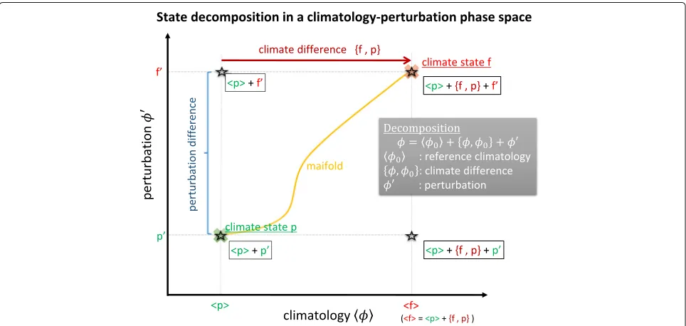
Let the large-scale state be denoted asφ, and its com-ponents of climatology and perturbation as φ and φ, respectively. There are several definitions of climatology, such as monthly long-term average. We discuss the defini-tion in the “Discussion” secdefini-tion. Here, we consider states under climatological equilibrium. Considering different climates, the climatology is further decomposed into the reference climatologyφ0and climate difference{φ,φ0}:
φ= φ0 + {φ,φ0} +φ, (1)
where the climate difference is expressed as {φ,φ0} = φ−φ0. For example, for future climate projections, the
future atmospheric state f can be decomposed into the present climatology p, future climate difference f,p, and future perturbationfso thatf = p +f,p+f.
by the spatial degree of freedom and the temporal degree of freedom. A schematic diagram of the phase space is shown in Fig. 1. Note that, although the phase space has a large number of dimensions, the schematic diagram is drawn as two-dimensional (climatology and perturbation) by a dimensionality reduction, e.g., the principal compo-nent analysis, for ease of understanding. The horizontal axis represents the subspaceVclim, whereφ ∈Vclim, and
the vertical axis represents the perpendicular complement spaceVclim⊥ , whereφ ∈Vclim⊥ . In the phase space, a point corresponds to a state; stateφis located at point(φ,φ), e.g., the cross marks in Fig. 1.
Uncertainty due to GCM errors
The statistical characteristics of the climatology and per-turbation are not independent of each other, since they are determined through their interactions with one another. Roughly speaking, they have a one-to-one correspon-dence, although there can be some ambiguities due to the possible existence of multi-equilibrium states. Here, we consider the statistical characteristics derived from the probability distribution function of possible states under the same climate condition, e.g., ensemble members in a GCM experiment; the characteristics of possible per-turbations under a climate do not depend on individual realizations. The one-to-one correspondence means that states can exist only in a manifold in the entire phase space because they are constrained by their relationship, as indicated by the yellow lines in Fig. 1.
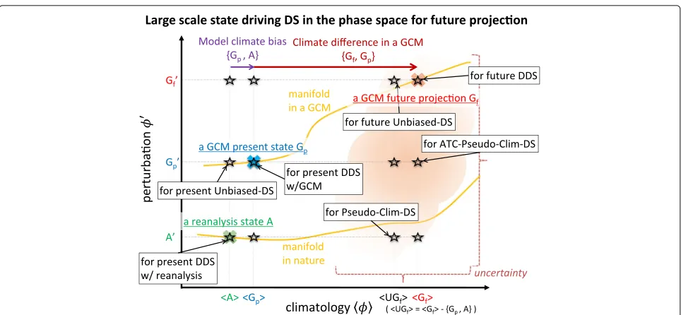
None of the numerical models are perfect, and the rep-resentation of interaction among components depends on the GCMs. That is, their relationship in GCMs may be distorted from that in nature. For example, an aqua-planet intermodel comparison shows a variety of relationships: there exist significant differences in precipitation systems compared to the differences in mean flow (Blackburn et al. 2013). The former is part of the perturbation, and the latter is part of the climatology. Because of the distorted relationship in a GCM, the states in a numerical simula-tion may exist in a different manifold from that of nature, as shown in Fig. 2. One remarkable point here is that there is a significant probability of a real atmospheric state exist-ing outside the region covered by numerical simulations in the phase space. DS driven only by the large-scale state in a distorted manifold can lead to an incorrect estimation of a regional climate.
Therefore, there is a need to explore a wider region than that covered by GCM simulations for the large-scale state driving the DS. The possible spuriousness in the relation-ship between the components in a GCM simulation is one of the causes of uncertainty in the estimation of the influence of climate change. If the GCM was perfect and we were confident about the perfection, the probability of the future state would be restricted only on the GCM’s manifold, which is identical to that in nature. This results in good projections with smaller uncertainties. However, GCMs have errors; thus, the true state would be outside of the GCM’s manifold because of the distorted constraint.
Fig. 2Schematic diagram of the large-scale state driving the downscaling simulations. Cross marks show the states realized by reanalysis and GCM simulations. Stars represent the possible large-scale states driving the downscaling simulations. The orange shaded area represents the range of uncertainty in the estimation or existence probability distribution of the future state. The yellow line shows the manifold corresponding to the relationship between climatology and perturbation
That is, the possible GCM errors spread the probabil-ity distribution. The region covered by simulations with a GCM in the phase space is limited to the spurious man-ifold. In fact, the trends in the CMIP5 historical runs (Taylor et al. 2012) are overconfident, and the observed trend is outside the range of the multi-model ensem-bles (van Oldenborgh et al. 2013). The bias-correcting methods produce states away from the GCM manifold, but the methods only shift the region in the phase space to another place and do not enlarge the region to be explored.
Reconstruction of large-scale states
In order to obtain large-scale states that are outside of the GCM’s manifold, we reconstruct the large-scale states. The climatology and perturbation from different states are not constrained in the distorted relationship of GCMs. Therefore, reconstruction by combining them produces large-scale states that are outside of the manifold. Let us consider the case of present and future states. Two com-ponents, the climatology and perturbations of the two states, are taken into account (Fig. 1). Considering these as independent components, four large-scale states can be obtained through their combinations, as illustrated by the stars in the diagram. It can be seen that two of these states are away from the spurious constraint. This independent treatment of the components achieves evaluation of states in a wider region of the phase space than the manifold of a GCM. The technical procedure to reconstruct the large-scale state is based on the Pseudo-Clim-DS in terms of
combining components from different states. However, in this conceptualization, the large-scale states are obtained in multiple ways. The previous DS methods, such as DDS, Unbiased-DS, and Pseudo-Clim-DS, are comprehensively involved.
For practical purposes, we often have three large-scale states: a reanalysis of the present climate stateA, a GCM of the present climate stateGp, and a GCM of the future
cli-mate stateGf (Fig. 2). Further, there are four climatologies: A,Gp,Gf, and UGf. The last one is the unbiased
future GCM climatology in which the climate bias of the model estimated under the present climate is removed:
UGf = Gf −
Gp,A
= A +Gf,Gp
. (2) For perturbations, there can be three states:A,Gp, and
be consistent, and tropical cyclones (TCs) should not be produced on the dry side of the Baiu front.
Our concept has another advantage in addition to wider coverage of the large-scale state in the phase space. The influence of changes in the individual components on the downscaled regional states can be examined. As a typical example, let us assume the following case: each differ-ence in the climatology and perturbation between the two states in the spurious manifold has opposite influences on the regional climate from each other, but not in nature’s manifold. In this case, the DS would lead to an under-estimation of the total influence. The above discussion indicates the importance of evaluating individual influ-ences in order to consider the total influence. Through a comparison of multiple DS simulations driven by the large-scale states that differ from one another by only one component, the influence of the individual components can be estimated. The regional stateψ obtained by DS depends on the large-scale stateφ:ψ =Dφ,φ, where
D is an operator representing the DS. The operator is interpreted as
ψ =Dφ,φ= φ +Pφ;φ+G[φ] , (3)
whereP is an operator representing modification of the large-scale perturbationφ under climatologyφby DS and G is one representing the variability generated or excited spontaneously under the given large-scale envi-ronment in the DS simulation. G consists of sub-GCM-grid-scale variability, which does not get resolved in GCM simulations, but gets resolved in DS simulations. The differences in the downscaled results with the differ-ent states, Df,f− Dp,p, can be divided into
Dp,p + {f,p}−Dp,pandDf,p + {f,p}−
Dp,p + {f,p}. The first represents the difference due to the change in climatology, and this is the quantity esti-mated with Pseudo-Clim-DS. This can be mainly inter-preted as the difference in the intensification and/or moving speed of a given perturbation under different cli-matologies in the DS simulations. The second represents the difference due to the difference in a given perturba-tion under the same climatology, e.g., the influence of the number of cyclones passing through the calculation domain.
The difference in the existing DS methods, clarified through our concept of constructing the large-scale state from independent components as their decomposition, is summarized in Table 1. In addition, the location of the states in the phase space is illustrated in Fig. 2. The concept can be described as a generalization of existing DS methods. Comparisons of the results obtained by different existing DS methods can be used to estimate the individual influence of the components. The influence of the difference in climatology can be estimated by com-paring the results obtained by DDS driven by reanalysis data and Pseudo-Clim-DS. A comparison can also be made between DDS driven by present climate GCM data and ATC-Pseudo-Clim-DS. The influence of perturbation can be examined by performing a comparison between the following DSs cases: (i) DDS with reanalysis data and present climate Unbiased-DS, (ii) future climate DDS and ATC-Pseudo-Clim-DS, and (iii) future climate Unbiased-DS and Pseudo-Clim-Unbiased-DS. A comprehensive evaluation of the results obtained by different DS methods in previous studies helps us understand the contribution of various
Table 1Possible large-scale states driving downscaling with reanalysis and GCM simulations in present and future climates
Perturbation A Gp Gf
Climatology
A A Gp− {Gp,A}
(= A + {A,A}) A + {A,A} +A A + {A,A} +Gp A + {A,A} +Gf
Present DDS (reanalysis) Present Unbiased-DS
Gp Gp
(= A + {Gp,A}) A + {Gp,A} +A A + {Gp,A} +Gp A + {Gp,A} +Gf
Present DDS (GCM)
UGf A+ {Gf,Gp} Gf− {Gp,A}
(= A + {Gf,Gp}) A + {Gf,Gp} +A A + {Gf,Gp} +Gp A + {Gf,Gp} +Gf
Pseudo-Clim-DS Future Unbiased-DS
Gf Gp+ {Gf,Gp} Gf
(= A + {Gf,A}) A + {Gf,A} +A A + {Gf,A} +Gp A + {Gf,A} +Gf
ATC-Pseudo-Clim-DS Future DDS
components to the total regional climate change in the future.
Demonstration of individual influences
In order to demonstrate an advantage of our concept, that is, the importance of estimating the individual influ-ences of changes in climatology and perturbation in the large-scale state on regional precipitation, we conduct a DS experiment based on the decomposition concept as an example. We simultaneously consider the influences of the two components on regional precipitation through a com-parison of three DS simulations. The experimental design is essentially the same as that of Yoshikane et al. (2012). However, our interest here is to focus on the decomposi-tion of the total influence into those of the climatology and perturbation, whereas the purpose of Yoshikane’s study was to verify the validity of the Pseudo-Clim-DS method for future DS projection.
The three DSs, i.e., the present climate DDS (Present-DDS) run, the future climate DDS (Future-(Present-DDS) run, and the ATC-Pseudo-Clim-DS run, are performed. The large-scale state driving the DS are denoted by Gp, Gf, and
Gp+{Gf,Gp}for the Present-DDS, Future-DDS, and
ATC-Pseudo-Clim-DS runs, respectively, where the states for the present and future climates in the GCM experiment are denoted by Gp and Gf, respectively. These can be
written as follows in the decomposed form:
Gp= Gp +
Gp,Gp
+Gp, (4)
Gf = Gp +
Gf,Gp
+Gf, (5)
Gp+
Gf,Gp
= Gp +
Gf,Gp
+Gp. (6)
The influence of climatology is estimated from the difference between the ATC-Pseudo-Clim-DS and Present-DDS runs,D[Gp,Gp + {Gf,Gp}]−D[Gp,Gp],
and that of the perturbation from the difference between the Future-DDS and ATC-Pseudo-Clim-DS runs,
D[Gf,Gp + {Gf,Gp}]−D[Gp,Gp + {Gf,Gp}].
In this demonstration, experiments involving 25-year-long time slices for the summer season (from June to September; referred to as JJAS) were performed under the present (1979 to 2003) and future (2075 to 2099) climate conditions in East Asia. Detailed descrip-tions of the experiment and the model are in the “Methods/Experimental” section. In the demonstration, the daily mean is used as the climatology of the large-scale state. We first obtained the monthly climatology by 25-year averaging. Next, we assumed that the monthly mean is the value on the 15th of each month and con-structed the daily climatology by linear interpolation of the monthly climatology. Here, we assume that climate change over 25 years is small enough to consider that the state is in climatological equilibrium. We ignore the bias in order to focus on demonstrating how individual
influences can be considered with the concept, although a formal assessment of future regional climate will need to consider the model climate bias. The analysis is conducted with the simulation result in domain 2 described in the “Methods/Experimental” section, except for the lateral nudging region.
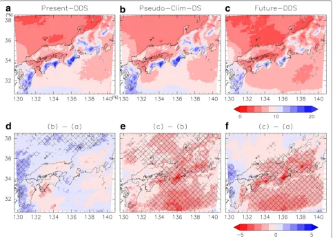
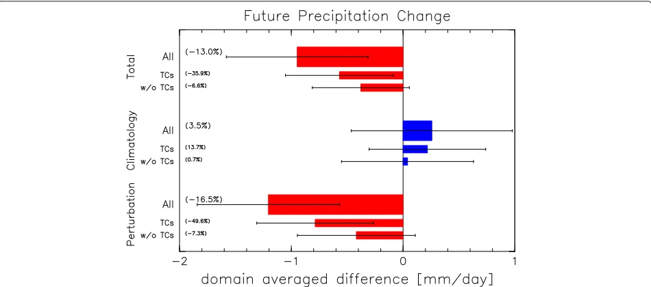
Figure 3 shows the summer climatology of the daily precipitation in the Present-DDS, ATC-Pseudo-Clim-DS, and Future-DDS runs. A large amount of precipitation is found in the high mountain areas near the Pacific Ocean. The precipitation in the Future-DDS is signifi-cantly weaker than that in the Present-DDS for the high-precipitation areas and the Pacific (Fig. 3f). The difference in precipitation resulting from climatology (Fig. 3d) is much smaller than the total difference. On the other hand, the difference resulting from perturbation is statistically significant (Fig. 3e). In another analysis by month, we confirmed significant differences due to perturbation in all months from June to September. This shows that the differences due to perturbation result in significant differ-ences in the DS simulations. Domain-averaged precipita-tion shows the same tendency (Fig. 4). The influences of climatology and perturbation have opposite signs. Since the individual influences have uncertainties, the magni-tude of each estimated change must be considered with some range of the uncertainty. In our result, the posi-tive change due to the climate difference is smaller than the negative change due to the perturbation difference in terms of absolute magnitude. Because of the uncer-tainty, there is a possibility that the magnitude relationship may reverse; that is, the positive change due to the cli-mate difference might be larger than the negative change due to the perturbation difference. Therefore, although the total difference in precipitation has a negative value in this experiment, it is possible for the total difference to be positive. This suggests that interpretations made by considering only the total change or the change in one component face the risk of misunderstanding the future regional climate. A simultaneous estimation considering the total and individual components is thus necessary. This result demonstrates the usefulness of the decompo-sition concept we propose in this study.
Fig. 3Horizontal distribution of the 25-year JJAS mean daily precipitation inathe Present-DDS,bPseudo-Clim-DS, andcFuture-DDS runs, and the difference due todthe climate difference (Pseudo-Clim-DS and Present-DDS),eperturbation difference (Future-DDS and Pseudo-Clim-DS), and
ftotal difference (future and Present-DDS runs). The hatched regions ineandfrepresent the area in which the difference is statistically significant with a 95% confidence level. The unit used is mm/day
this region. In the GCM future projection run used to drive the DS, the number of TCs is smaller than that in the present run (Murakami et al. 2012). The fewer TCs in future climate is also indicated by pre-vious studies using other GCMs (e.g., Knutson et al. 2015; Roberts et al. 2015). The smaller number of TCs in the future is consistent with the smaller amount of precipitation. We examine the precipitation associated with the TCs. Cyclone track detection is described in the “Methods/Experimental” section. We define TC precipi-tation as the precipiprecipi-tation within a distance of 1000 km from the center of a TC. The contribution of the TC precipitation to the total precipitation change is larger than that of the non-TC precipitation, as shown in Fig. 4 (top). The precipitation change associated with TCs is primarily attributed to the perturbation difference. This is consistent with the fact that the number of TCs pro-jected in the future perturbation is much smaller than that in the present. Increasing TC precipitation due to the
climate difference can be observed (Fig. 4, middle). This implies that TCs are intensified in the future climatology compared to the present. This result is consistent with previous studies (e.g., Ying et al. 2012; Christensen et al. 2013). It is observed that the decreasing trend in the non-TC precipitation is mainly attributed to the perturbation difference. The change is dominant in June, and it is not as large in other months. The smaller non-TC precipitation in June is consistent with the slower northward movement of the Baiu front in the GCM future projection than in the present (Kusunoki et al. 2011; Kanada et al. 2012). On the other hand, the influence of climatology on the non-TC precipitation is quite small.
Discussion
Fig. 4Contribution of each component to domain-averaged 25-year JJAS mean daily precipitation difference. The total difference, the difference due to climate difference, and that due to perturbation are shown at the top, middle, and bottom, respectively, on the vertical axis. These differences are further divided into ones associated with tropical cyclones and other factors. The error bars represent the 95% confidence interval of Welch’s statistics. The percentages represent the ratios of the difference to the total precipitation in the Present-DDS run
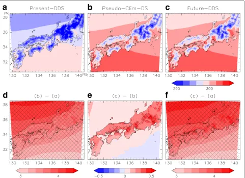
dominant contribution of the climate difference relative to the difference in the perturbation as shown in Fig. 5, and the perturbation difference is dominant in the precipita-tion change. This suggests that applying this concept to various cases and fields is important in order to interpret the regional future projections.
In the analysis discussed in the demonstration, non-linear interaction between climatology and perturbation in the DS simulation, i.e., nonlinearity in operator D, is not considered. Actually, operatorDhas some degree of nonlinearity, and the estimation of individual influences would be contaminated because of the nonlinearity. The comparison betweenDp,p +f,p−Dp,pand
Df,p +f,p−Df,porDf,p−Dp,p
andDf,p +f,p−Dp,p +f,pgives us a hint of the nonlinearity. The nonlinearity can also be inves-tigated by comparing multiple DS simulations based on the strategy. Adachi et al. (2017) proposed a procedure to extract the interaction effect and showed that the interac-tion can have a greater influence on heavier precipitainterac-tion, whereas Kröner et al. (2016) showed that the nonlinear-ity could be negligible in their case. Careful considerations for the nonlinearity are necessary in each case.
In the DS experiment in this study, climatology is defined as the daily interpolated climatological monthly mean. Interannual and inter-seasonal variability, such as ENSO, is included in the perturbation. There are vari-ations in the definition of climatology. For instance, although seasonal and daily changes can be included in climatology, they can also be treated as perturbations.
These components should be defined based on the purpose of the study. In addition, the climatology– perturbation decomposition is just one of several possi-ble decompositions. In order to understand the influences of other components, different decompositions would be appropriate. For instance, Adachi et al. (2012) investigated the impact of urbanization on regional climate with a Pseudo-Clim-DS experiment with the present and future urbanization conditions. Kröner et al. (2016) decomposed the future change into changes due to three effects (the large-scale thermodynamic effect, lapse-rate effect, and large-scale circulation) and other remaining effects. Com-parisons between the individual impacts obtained through such experiments would give us a better understanding of future change. Here, it should be noted that dynamical or other balances should be considered in the independent treatment of the decomposed components; otherwise, the variability in DS simulations could be violated because of non-physical factors. In addition, we consider that other quantities (not just the mean) are important in climate change, such as quantities related to extremes, although we discuss only the mean as an example.
Fig. 5Horizontal distribution of the 25-year JJAS mean 2-m temperature inathe Present-DDS,bPseudo-Clim-DS, andcFuture-DDS runs, and the difference due todthe climate difference (Pseudo-Clim-DS and Present-DDS),eperturbation difference (Future-DDS and Pseudo-Clim-DS), and
ftotal difference (future and Present-DDS runs). The hatched region ineandfrepresents the area in which the difference is statistically significant with a 95% confidence level
of small-scale variability. In addition to considering the uncertainty due to the GCM’s errors by including a wider coverage of possible large-scale states, it is important to consider the uncertainty due to the RCM’s errors, which can be evaluated by multi-RCM experiments.
Conclusions
We conceptualized dynamical downscaling and presented a perspective on downscaling for regional climate stud-ies. In this study, we provided a comprehensive view of the previous downscaling methods based on reconstruc-tion of the large-scale state driving DS from indepen-dent decomposed components, such as climatology and perturbation.
The concept of the reconstruction of the decomposed components provides not only a comprehensive view of DS but also a strategy for coordinated experimental design for future regional climate studies. We can obtain the large-scale states from a wider region in the phase
space, whereas only the states in the spurious manifold in the phase space distorted by interactions between the components due to a GCM error are obtained by the previous individual DS methods. Furthermore, we can estimate the individual influences of the change in the components of the large-scale state on the downscaled regional climate. The importance of the simultaneous consideration of individual influences is demonstrated by a DS experiment. We estimated the influence of both the climatology and perturbation change on the future pre-cipitation simultaneously and found that the influence of the perturbation can be significant, as well as that of the climatology.
results. The region in the phase space covered by multi-model and/or multi-physics ensemble GCM simulations is larger than that of a single-model and single-physics case. However, the manifolds of the different GCMs can be isolated from one another, and the covered region was discretely distributed. In order to understand the charac-teristics of the output of a nonlinear operator, inputs that are not only widely but also evenly distributed are gen-erally preferable to those that are locally concentrated in some places because the operator has local linearity. In this sense, in order to assess the uncertainty more reli-ably, DS simulations driven not only by the large-scale states obtained by ensemble GCM simulations but also by reconstructed states from components of the ensembles should be performed. In addition to the total uncertainty, an estimation of the individual uncertainty associated
with each component is as necessary as the absolute magnitude of the influence due to individual compo-nents. The contribution of each component differs in its uncertainty and absolute magnitude.
Methods/Experimental
Experimental settings
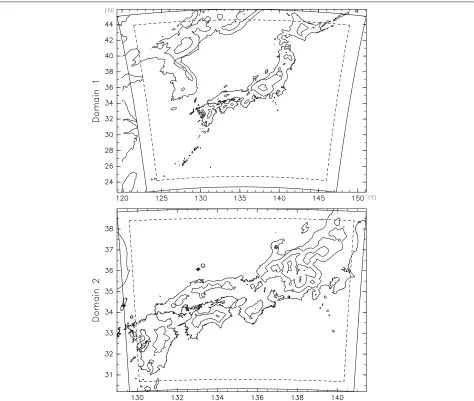
In the demonstration, the total 25-year summer time data was obtained by performing five-day integrations over-lapping a one-day spin-up term. Two nested domains are used for DS: domain 1, which is 2520×2520 km2 with a 7.5 km grid spacing, and domain 2 nested in domain 1, which is 1080×960 km2with a 2.5 km grid spacing; both domains have the same domain center of 135.2 °E and 34.7 °N (Fig. 6) The numbers of vertical layers are 36 and 60 for domains 1 and 2, respectively.
Regional model
The regional model used for the DS experiment is the Scalable Computing for Advanced Library and Environ-ment Regional model (SCALE-RM) (Nishizawa et al. 2015; Sato et al. 2015; available at http://scale.aics.riken.jp). A six-category one-moment bulk scheme (Tomita 2008), ak-distribution scheme (Sekiguchi and Nakajima 2008), the MYNN level 2.5 scheme (Nakanishi and Niino 2009), a similarity scheme (Beljaars and Holtslang 1991; Wilson 2001), a diffusion and bucket scheme, and a single-layer urban canopy model (Kusaka et al. 2001) are used to rep-resent cloud microphysical processes, radiation transfer, planetary boundary layer turbulence, surface flux, land processes, and urban processes, respectively.
Large-scale state
The large-scale state obtained by a 20-km resolution Atmospheric Model Intercomparison Project (AMIP)-type experiment with the Meteorological Research Insti-tute atmospheric GCM (MRI-AGCM) (Mizuta et al. 2012) is used to drive the DS. In the AGCM experiment, the sea surface temperature (SST) of HadISST1 (Rayner et al. 2003) is prescribed in the present climate run (Mizuta et al. 2012), and the multi-model ensemble averaged SST of the CMIP5 (Taylor et al. 2012) coupled-GCM runs with the Representative Concentration Pathways (RCP) 8.5 scenario is prescribed in the future climate run (Mizuta et al. 2014).
Cyclone track detection
The cyclone track is detected using the method proposed by Adachi and Kimura (2007), and a TC is defined as a cyclone that comes from south of 25 °N. The corre-sponding cyclones in the GCM simulation are used for the TC determination, since the domain for the DS is not wide enough for the determination. The numbers of TCs entering the domain of analysis are 150, 158, and 90, in the Present-DDS, ATC-Pseudo-Clim-DS, and Future-DDS runs, respectively. Here, the numbers are different for the Present-DDS and ATC-Pseudo-Clim-DS runs because of slight differences in TC tracks in the outer domain.
Abbreviations
AGCM: Atmospheric general circulation model; AMIP: Atmospheric model intercomparison project; ATC: Assumed true climate; DS: Downscaling; DDS: Direct downscaling; GCM: General circulation model or Global climate model; JJAS: June to September; MRI: Meteorological Research Institute;
Pseudo-Clim-DS: Pseudo climate change downscaling; RCM: Regional climate model; SST: Sea surface temperature; TC: Tropical cyclones
Acknowledgements
The MRI-AGCM3.2S data were provided by the Program for Risk Information on Climate Change (SOUSEI) of the Ministry of Education, Culture, Sports, Science, and Technology (MEXT) of Japan conducted by the Meteorological Research Institute (MRI). This research used computational resources of the K computer provided by the RIKEN Advanced Institute for Computational Science through the HPCI System Research project (Project ID:hp160119). The
analysis and visualization in this study was conducted using the products of the GFD-Dennou Club (http://www.gfd-dennou.org/).
Funding
This work was supported by the FOCUS Establishing Supercomputing Center of Excellence and JST CREST Grant Number JPMJCR1312, Japan.
Availability of data and materials
The regional model for the downscaling calculation in this study was constructed using SCALE, which is freely available at https://scale.aics.riken.jp/ download/index.html under the 2-Clause BSD license. The model code used is based on SCALE-RM version 4.2.5 including some improvements such as the usability of the microphysics scheme. The model code and the set of configuration parameters are available from the corresponding author upon reasonable request. The pre-process code that generates the boundary conditions for SCALE-RM from the MRI-AGCM3.2 data and the post analysis code used in this study are also available from the corresponding author. The downscaling data by SCALE-RM is deposited in local storage at RIKEN/AICS. It is available from the corresponding author upon reasonable request. The MRI-AGCM data was provided to the authors by MRI under a given condition that the authors can use the MRI-AGCM data only for the current and related studies. The data is not publicly available. However, upon reasonable request with regards to this study, the data are provided from MRI with the permission of MRI. In this case, contact person is the corresponding author.
Authors’ contributions
SN, SAA, YK, and HT designed the research. SN, SAA, TY, and KA carried out the downscaling simulation. SN, SAA, TY, KA, and RY analyzed the data. SN, SAA, YK, and HT wrote the paper. YK, HY, and HT supervised the research. All authors contributed to discussions of the results and read and approved the manuscript.
Ethics approval and consent to participate
Not applicable.
Consent for publication
Not applicable.
Competing interests
The authors declare that they have no competing interests.
Publisher’s Note
Springer Nature remains neutral with regard to jurisdictional claims in published maps and institutional affiliations.
Author details
1RIKEN Advanced Institute for Computational Science, 7-1-26
Minatojima-minami-machi, Chuo-ku, Kobe, Hyogo 650-0047, Japan.2Research Center for Urban Safety and Security, Kobe University, 1-1 Rokkodai-cho, Nada-ku, Kobe, Hyogo 657-8501, Japan.
Received: 8 May 2017 Accepted: 13 December 2017
References
Adachi SA, Kimura F (2007) A 36-year climatology of surface cyclogenesis in East Asia using high-resolution reanalysis data. SOLA 3:113–116. doi:10.2151/sola.2007-029
Adachi SA, Kimura F, Kusaka H, Inoue T, Ueda H (2012) Comparison of the impact of global climate changes and urbanization on summertime future climate in the Tokyo metropolitan area. J Appl Meteorol
Climatol:1441–1454. doi:10.1175/JAMC-D-11-0137.1
Adachi SA, Nishizawa S, Yoshida R, Yamaura T, Ando K, Yashiro H, Kajikawa Y, Tomita H (2017) Contributions of changes in climatology and perturbation and the resulting nonlinearity to regional climate change. Nat Commun 8(2224). doi:10.1038/s41467-017-02360-z
Beljaars ACM, Holtslag AAM (1991) Flux parameterization over land surfaces for atmospheric models. J Appl Meteorol 30:327–341. http://doi.org/10.1175/ 1520-0450(1991)030%3C0327:FPOLSF%3E2.0.CO;2
Blackburn M, Williamson DL, Nakajima K, Ohfuchi W, Takahashi YO, Hayashi Y-Y, Nakamura H, Ishiwatari M, McGregor JL, Borth H, Wirth V, Frank H, Bechtold P, Wedi NP, Tomita H, Satoh M, Zhao M, Held IM, Suarez MJ, Lee M-I, Watanabe M, Kimoto M, Liu Y, Wang Z, Molod A, Rajendran K, Kitoh A, Stratton R (2013) The aqua-planet experiment (APE): Control SST simulation. J Meteorol Soc Japan Ser II 91A:17–56. doi:10.2151/jmsj. 2013-A02
Christensen JH, Kumar KK, Aldrian E, An S-I, Cavalcanti IFA, de Castro M, Dong W, Goswami P, Hall A, Kanyanga JK, Kitoh A, Kossin J, Lau N-C, Renwick J, Stephenson DB, Xie S-P, Zhou T (2013) Climate phenomena and their relevance for future regional climate change. In: Climate Change 2013: The Physical Science Basis. Contribution of Working Group I to the Fifth Assessment Report of the Intergovernmental Panel on Climate Change. Cambridge University Press, Cambridge. Chap. 14
Cook KH, Vizy EK (2008) Effects of twenty-first-century climate change on the Amazon rain forest. J Climate 21:542–560. doi:10.1175/2007JCLI1838.1 Déqué M, Somot S, Sanchez-Gomez E, Goodess CM, Jacob D, Lenderink G,
Christensen OB (2012) The spread amongst ensembles regional scenarios: regional climate models, driving general circulation models and interannual variability. Clim Dyn 38(5):951–964. doi:10.1007/s00382-011-1053-x Dickinson RE, Errico RM, Giorgi F, Bates GT (1989) A regional climate model for
the western United States. Clim Change 15:383–422. doi:10.1007/BF00240465 Done JM, Holland GJ, Bruyère CL, Leung LR, Suzuki-Parker A (2015) Modeling
high-impact weather and climate: lessons from a tropical cyclone perspective. Clim Change 129:381–395. doi:10.1007/s10584-013-0954-6 Evans JP, Ji F, Lee C, Smith P, Argüeso D, Fita L (2014) Design of a regional
climate modelling projection ensemble experiment—NARCliM. Geosci Model Dev 7:621–629. doi:10.5194/gmd-7-621-2014
Giorgi F, Bates GT (1989) The climatological skill of a regional model over complex terrain. Mon Wea Rev 117:2325–2347. http://doi.org/10.1175/ 1520-0493(1989)117%3C2325:TCSOAR%3E2.0.CO;2
Giorgi F, Shields C (1999) Tests of precipitation parameterizations available in latest version of NCAR Regional Climate Model (RegCM) over continental United States. J Geophys Res 104:6353–6375. doi:10.1029/98JD01164 Holland GJ, Done J, Bruyere C, Cooper C, Suzuki A (2010) Model investigations
of the effects of climate variability and change on future Gulf of Mexico tropical cyclone activity. In: Proc. Offshore Technology Conf. Offshore Technology Conference, Texas. Offshore Technology Conference. doi:10.4043/20690-MS
Jin JM, Wang SY, Gillies RR (2011) An improved dynamical downscaling for the western United States. In: Blanco J (ed). Climate Change: Research and Technology for Adaptation and Mitigation. InTech, Rijeka Croatia. pp 23–38. Chap. 2. doi:10.5772/22991
Jones RG, Murphy JM, Noguer M (1995) Simulation of climate change over Europe using a nested regional-climate model. Part I: Assessment of control climate, including sensitivity to location of lateral boundaries. Quart J R Meteorol Soc 121:1413–1449. doi:10.1002/qj.49712152610 Kanada S, Nakano M, Kato T (2012) Projections of future changes in
precipitation and the vertical structure of the frontal zone during the Baiu season in the vicinity of Japan using a 5-km-mesh regional climate model. J Meteorol Soc Japan 90A:65–86. doi:10.2151/jmsj.2012-A03
Kato H, Nishizawa K, Hirakuchi H, Kadokura S, Oshima N, Giorgi F (2001) Performance of RegCM2.5/NCAR-CSM nested system for the simulation of climate change in East Asia caused by global warming. J Meteorol Soc Japan 79:99–121. doi:10.2151/jmsj.79.99
Kawase H, Yoshikane T, Hara M, Ailikun B, Kimura F, Yasunari T (2008) Downscaling of the climatic change in the Mei-yu rainband in East Asia by a pseudo climate simulation method. SOLA 4. doi:10.2151/sola.2008-019 Kawase H, Yoshikane T, Hara M, Kimura F, Yasunari T, Ailikun B, Ueda H, Inoue T
(2009) Intermodel variability of future changes in the Baiu rainband estimated by the pseudo global warming downscaling method. J Geophys Res 114(D24110). doi:10.1029/2009JD011803
Kimura F, Kitoh A (2007) Downscaling by pseudo global warming method. The final report of ICCAP. Research Institute for Humanity and Nature, Kyoto Knutson TR, Sirutis JJ, Zhao M, Tuleya RE, Bender M, Vecchi GA, Villarini G,
Chavas D (2015) Global projections of intense tropical cyclone activity for the late twenty-first century from dynamical downscaling of CMIP5/RCP4.5 scenarios. J Climate 28(18):7203–7224. doi:10.1175/JCLI-D-15-0129.1 Kröner N, Kotlarski S, Fischer E, Lüthi D, Zubler E, Schär C (2016) Separating
climate change signals into thermodynamic, lapse-rate and circulation
effects: theory and application to the European summer climate. Clim Dyn. doi:10.1007/s00382-016-3276-3
Kusaka H, Kondo H, Kikegawa Y, Kimura F (2001) A simple single-layer urban canopy model for atmospheric models: comparison with multi-layer and slab models. Bound-Layer Meteorol 101(3):329–358.
doi:10.1023/A:1019207923078
Kusunoki S, Mizuta R, Matsueda M (2011) Future changes in the East Asian rain band projected by global atmospheric models with 20-km and 60-km grid size. Clim Dyn 37:2481–2493. doi:10.1007/s00382-011-1000-x
Mearns O, Giorgi F, McDaniel L, Shields C (1995) Analysis of daily variability of precipitation in a nested regional climate model: comparison with observations and doubled CO2 results. Global Planet Change 10:55–78. doi:10.1016/0921-8181(94)00020-E
Mearns L. O, Sain S, Leung LR, Bukovsky MS, McGinnis S, Biner S, Caya D, Arritt RW, Gutowski W, Takle E, Snyder M, Jones RG, Nunes AMB, Tucker S, Herzmann D, McDaniel L, Sloan L (2013) Climate change projections of the North American Regional Climate change Assessment Program (NARCCAP). Clim Change 120:965–975. doi:10.1007/s10584-013-0831-3 Misra V, Kanamitsu M (2004) Anomaly nesting: a methodology to downscale
seasonal climate simulations from AGCMs. J Climate 17:3249–3262. http:// doi.org/10.1175/1520-0442(2004)017%3C3249:ANAMTD%3E2.0.CO;2 Mizuta R, Yoshimura H, Murakami H, Matsueda M, Endo H, Ose T, Kamiguchi K,
Hosaka M, Sugi M, Yukimoto S, Kusunoki S, Kitoh A (2012) Climate simulations using MRI-AGCM3.2 with 20-km grid. J Meteorol Soc Japan 90A:233–258. doi:10.2151/jmsj.2012-A12
Mizuta R, Arakawa O, Ose T, Kusunoki S, Endo H, Kitoh A (2014) Classification of CMIP5 future climate responses by the tropical sea surface temperature changes. SOLA 10:167–171. doi:10.2151/sola.2014-035
Murakami H, Wang Y, Yoshimura H, Mizuta R, Sugi M, Shindo E, Adachi Y, Yukimoto S, Hosaka M, Kusunoki S, Ose T, Kitoh A (2012) Future changes in tropical cyclone activity projected by the new high-resolution MRI-AGCM. J Clim 25:3237–3260. doi:10.1175/JCLI-D-11-00415.1
Nakanishi M, Niino H (2009) Development of an improved turbulence closure model for the atmospheric boundary layer. J Meteorol Soc Japan 87:895–912. doi:10.2151/jmsj.87.895
Nishizawa S, Yashiro H, Sato Y, Miyamoto Y, Tomita H (2015) Influence of grid aspect ratio on planetary boundary layer turbulence in large-eddy simulations. Geosci Model Dev 8:3393–3419. doi:10.5194/gmd-8-3393-2015
Patricola CM, Cook KH (2010) Northern African climate at the end of the twenty-first century: an integrated application of regional and global climate models. Clim Dyn 35:193–212. doi:10.1007/s00382-009-0623-7 Rasmussen R, Liu C, Ikeda K, Gochis D, Yates D, Chen F, Tewari M, Barlage M,
Dudhia J, Yu W, Miller K (2011) High-resolution coupled climate runoff simulations of seasonal snowfall over Colorado: a process study of current and warmer climate. J Clim 24:3015–3048. doi:10.1175/2010JCLI3985.1 Rayner NA, Parker DE, Horton EB, Folland CK, Alexander LV, Rowell DP, Kent EC,
Kaplan A (2003) Global analyses of sea surface temperature, sea ice, and night marine air temperature since the late nineteenth century. J Geophys Res 108(D14). doi:10.1029/2002JD002670
Roberts MJ, Vidale PL, Mizielinski MS, Demory M-E, Schiemann R, Strachan J, Hodges K, Bell R, Camp J (2015) Tropical cyclones in the UPSCALE ensemble of high-resolution global climate models. J Climate 28(2):574–596. doi:10.1175/JCLI-D-14-00131.1
Rowell DP, Jones RG (2006) Causes and uncertainty of future summer drying over Europe. Clim Dyn 27:281–299. doi:10.1007/s00382-006-0125-9 Rummukainen M, Rockel B, Bärring L, Christensen JH, Reckermann M (2015)
Twenty-first-century challenges in regional climate modeling. Bull Amer Meteorol Soc 96:135–138. doi:10.1175/BAMS-D-14-00214.1
Sato T, Kimura F, Kitoh A (2007) Projection of global warming onto regional precipitation over Mongolia using a regional climate model. J Hydrol 333:144–154. doi:10.1016/j.jhydrol.2006.07.023
Sato Y, Nishizawa S, Yashiro H, Miyamoto Y, Kajikawa Y, Tomita H (2015) Impacts of cloud microphysics on trade wind cumulus: which cloud microphysics processes contribute to the diversity in a large eddy simulation? Prog Earth Planet Sci 2. doi:10.1186/s40645-015-0053-6 Schär C, Frei C, Lüthi D, Davies HC (1996) Surrogate climate-change scenarios
for regional climate models. Geophys Res Lett 23:669–672. doi:10.1029/96GL00265
Takayabu I, Kanamaru H, Dairaku K, Benestad R, von Storch H, Christensen JH (2016) Reconsidering the quality and utility of downscaling. J Meteorol Soc Japan Ser II 94A:31–45. doi:10.2151/jmsj.2015-042
Taylor KE, Stouffer RJ, Meehl GA (2012) An overview of CMIP5 and the experiment design. Bull Am Meteorol Soc 93:485–498. doi:10.1175/BAMS-D-11-00094.1
Tomita H (2008) New microphysical schemes with five and six categories by diagnostic generation of cloud ice. J Meteorol Soc Japan 86A:121–142. doi:10.2151/jmsj.86A.121
van der Linden P, Mitchell FB (2009) ENSEMBLES: climate change and its impacts: summary of research and results from the ENSEMBLES project. technical report. Met Office Hadley Centre, FitzRoy Road, Exeter, EX1 3PB, U. K
van Oldenborgh GJ, Reyes FJD, Drijfhout SS, Hawkins E (2013) Reliability of regional climate model trends. Environ Res Lett 8.
doi:10.1088/1748-9326/8/1/014055
Wakazuki Y, Rasmussen R (2015) Incremental dynamical downscaling for probabilistic analysis based on multiple GCM projections. Geophys Res Lett 42:10847–10855. doi:10.1002/2015GL066242
Walsh K, McGregor JL (1995) January and July climate simulations over the Australian region using a limited-area model. J Clim 8:2387–2403. http:// doi.org/10.1175/1520-0442(1995)008%3C2387:JAJCSO%3E2.0.CO;2 Wang Y, Leung LR, McGregor JL, Lee D-K, Wang W-C, Ding Y, Kimura F (2004)
Regional climate modeling: Progress, challenges and prospects. J Meteorol Soc Japan 82:1599–1628. doi:10.2151/jmsj.82.1599
Wilson DK (2001) An alternative function for the wind and temperature gradients in unstable surface layers. Bound-Layer Meteorol 99:151–158. doi:10.1023/A:1018718707419
Wu W, Lynch AH (2000) Response of the seasonal carbon cycle in high latitudes to climate anomalies. J Geophys Res 105(D18):22897–22908. doi:10.1029/2000JD900340
Xu Z, Yang Z-L (2012) An improved dynamical downscaling method with GCM bias corrections and its validation with 30 years of climate simulations. J Clim 25:6271–6286. doi:10.1175/JCLI-D-12-00005.1
Ying M, Knutson TR, Kamahori H, Lee T-C (2012) Impacts of climate change on tropical cyclones in the western north pacific basin. part II: Late twenty-first century projections. Tropical Cyclone Res Rev 1:231–241
Yoshikane T, Kimura F, Kawase H, Nozawa T (2012) Verification of the performance of the pseudo-global-warming method for future climate changes during June in East Asia. SOLA 8:133–136.