www.geosci-model-dev.net/8/579/2015/ doi:10.5194/gmd-8-579-2015
© Author(s) 2015. CC Attribution 3.0 License.
A statistical downscaling method for daily air temperature in
data-sparse, glaciated mountain environments
M. Hofer1, B. Marzeion1, and T. Mölg2
1Institute of Meteorology and Geophysics, University of Innsbruck, Innsbruck, Austria
2Climate System Research Group, Institute of Geography, Friedrich-Alexander-University Erlangen-Nuremberg (FAU), Nuremberg, Germany
Correspondence to: M. Hofer ([email protected])
Received: 12 February 2013 – Published in Geosci. Model Dev. Discuss.: 17 May 2013 Revised: 11 February 2015 – Accepted: 19 February 2015 – Published: 12 March 2015
Abstract. This study presents a statistical downscaling (SD) method for high-altitude, glaciated mountain ranges. The SD method uses an a priori selection strategy of the predictor (i.e., predictor selection without data analysis). In the SD model validation, emphasis is put on appropriately consid-ering the pitfalls of short observational data records that are typical of high mountains. An application example is shown, with daily mean air temperature from several sites (all in the Cordillera Blanca, Peru) as target variables, and reanalysis data as predictors. Results reveal strong seasonal variations of the predictors’ performance, with the maximum skill evi-dent for the wet (and transitional) season months January to May (and September), and the lowest skill for the dry sea-son months June and July. The minimum number of obser-vations (here, daily means) required per calendar month to obtain statistically significant skill ranges from 40 to 140. With increasing data availability, the SD model skill tends to increase. Applied to a choice of different atmospheric reanal-ysis predictor variables, the presented skill assessment iden-tifies only air temperature and geopotential height as signif-icant predictors for local-scale air temperature. Accounting for natural periodicity in the data is vital in the SD proce-dure to avoid spuriously high performances of certain pre-dictors, as demonstrated here for near-surface air tempera-ture. The presented SD procedure can be applied to high-resolution, Gaussian target variables in various climatic and geo-environmental settings, without the requirement of sub-jective optimization.
1 Introduction
Ongoing developments in atmospheric modeling have made available various long-term, temporally high-resolution at-mospheric data sets for the entire globe. However, these data sets are still restricted in terms of spatial resolutions, such that their immediate application to study regional and lo-cal climate is not recommended. In fact, global atmospheric models often miss significant processes that characterize lo-cal weather and climate. This slo-cale discrepancy between the global atmospheric models and the local-scale variability is particularly problematic for areas of complex topography, such as glacier-covered mountains. So-called downscaling methods bridge the gap between the available data from the global atmospheric models and the required local-scale infor-mation (for an overview see, e.g., Christensen et al., 2007). Generally two types of downscaling exist, namely, dynam-ical downscaling (e.g., Hill, 1968; Giorgi and Bates, 1989; Mearns et al., 2003), and statistical downscaling (SD) (e.g., Klein et al., 1959; Wilby et al., 2004; Benestad et al., 2008). Since the early development of both downscaling classes a variety of different models and approaches have emerged.
C O
R D
. N
E G
R A
C O
R D
. B
L A
N C
A Chimbote
R io
Sa nta
Huaraz AWS1,AWS2
AWS3
k
City Glaciers
Investigation Sites
0 10 20 30 40 m
Rivers
8°50'S
9°10'S
78°00'W
77°20'W
10°10'S 8°30'S
77°40'W
Watershed Rio Santa
Figure 1. The map shows the Rio Santa watershed with the Cordillera Blanca mountain range and the positions of AWS1, AWS2 and AWS3 (mentioned in the text). Also indicated is the 1990 glacier extent (gray shaded area; Georges, 2004).
studies (e.g., Winkler et al., 1997; Cavazos and Hewitson, 2005) have systematically assessed the relevance of different predictors in terms of variable types, spatial area, or predic-tor model. Wilby et al. (2002) propose a promising solution by providing regression-based, automated tools for predictor selection in SD (see also Wilby and Dawson, 2007; Hessami et al., 2008). Yet these methods are suitable only if the ob-servational database for model calibration is relatively large (e.g., daily time series for more than a decade). Moreover, the transfer of appropriate predictors amongst different sites or variables is usually not possible for data-based selections. The problem of predictor and model selection is well known also beyond the field of atmospheric sciences (e.g., Zucchini, 2000; Hastie et al., 2001; Bair et al., 2006).
This study presents an SD method for high-altitude, moun-tainous sites. The SD method is designed to (i) appropriately consider the pitfalls of short (i.e., few years) observational time series in the model training and evaluation; (ii) provide an objective tool for model and predictor assessment and se-lection; and to (iii) be easily transferred to different sites and target variables, without the requirement of subjective opti-mization. The SD method as presented here is restricted to Gaussian target variables. It is comprehensible and of min-imum complexity. We show an application example of the SD method to quantify the skill of reanalysis data as pre-dictors for local-scale, daily air temperature in the tropical Cordillera Blanca. Study site, target variables and large-scale predictors are described in the next section (Sect. 2). Sec-tion 3 gives a comprehensive descripSec-tion of the SD model. The results of the application example, based on a priori pre-dictor selection strategy, are presented in Sects. 4.1 to 4.3. In Sects. 4.4 and 4.5 we show applications of the SD model for various predictor variables, and at different timescales. Sec-tion 5 shows limitaSec-tions and possible extensions of the SD model. The study’s main findings are summarized in Sect. 6.
2 Application example 2.1 Study site
The SD model will be presented on the basis of a case study that focuses on the Cordillera Blanca. The Cordillera Blanca is a glaciated mountain range located in the north-ern Andes of Peru (Fig. 1). It harbors 25 % of all tropical glaciers with respect to surface area (Kaser and Osmaston, 2002). Glaciers in the Cordillera Blanca have been shrink-ing since their last maximum extent in the late 19th century (e.g., Ames, 1998; Georges, 2004; Silverio and Jaquet, 2005; Schauwecker et al., 2014), and have significantly shaped the socioeconomic development in the region. During the 20th century, a series of the history’s most catastrophic glacier disasters occurred (i.e., outburst floods and avalanches; e.g., Carey, 2005, 2010). Also, Cordillera Blanca glaciers have important positive impacts for water availability in industry, agriculture, and households. In particular, Cordillera Blanca glaciers contribute to balancing the strong runoff seasonal-ity in the extensively populated Rio Santa valley (e.g., Mark and Seltzer, 2003; Kaser et al., 2003; Juen, 2006; Juen et al., 2007; Kaser et al., 2010).
automatic weather stations (AWSs) has been installed at and nearby glaciers in the Cordillera Blanca since 1999. The pri-mary goal of the measurement network was to provide high-resolution data for glacier mass balance, and runoff modeling (Juen et al., 2007). Maintaining the AWSs to provide contin-uous and reliable atmospheric time series has represented a logistical and technical challenge. Field work has been costly in terms of time and materials, since the AWSs are located at very high altitudes (between 4700 and 5100 m a.s.l.), and in remote areas. Further problems also include instrument theft and natural hazards (Juen, 2006). Due to these difficulties of providing long-term and reliable measurement series from these sites, SD methods have been investigated that are able to provide useful results also on the basis of limited mea-surement availability. Hofer et al. (2010) presented a compre-hensive SD modeling procedure for extending the short-term AWS time series backwards in time. They used sub-daily air temperature and specific humidity as the target variables, and reanalysis data as the large-scale predictors. Hofer et al. (2010) found that the SD model skill largely varies as a func-tion of season and time of day, and emphasized uncertainty in the exact choice of the mixed-field predictors variables. Hofer et al. (2012) used a simpler methodology that is based on single linear regression, in order to determine the opti-mum reanalysis data set for air temperature in the Cordillera Blanca.
2.2 The predictands: daily mean air temperature from different sites
The target variables (predictands) of the present study are daily mean air temperature time series measured at three dif-ferent AWSs in the Cordillera Blanca (hereafter referred to as AWS1, AWS2, and AWS3). AWS1, AWS2 and AWS3 include the longest time series available from all AWSs in-stalled in the Cordillera Blanca to date. Yet the measuring periods are still relatively short, ranging from July 2006 to July 2012 (AWS1), to August 2011 (AWS2), and to Decem-ber 2009 (AWS3), with 3 months of missing data at AWS2. Below, we refer to period 1 as the common period of avail-able data for all three AWSs (i.e., July 2006 to Decem-ber 2009), and to period 2 as the longest measurement pe-riod (at AWS1, i.e., July 2006 to July 2012). AWS1, AWS2, and AWS3 are situated in the vicinity of retreating glacier tongues on rocky terrain (glacial polish and moraines), at 5050, 4825, and 4950 m a.s.l., respectively. Whereas AWS1 and AWS2 are located at only about two kilometers distance in the Paron valley (northern Cordillera Blanca), AWS3 is located approximately 100 km further southward in the Shal-lap valley (to the west of Huaraz, the capital of the Ancash region). The locations of AWS1, AWS2, and AWS3 are indi-cated in Fig. 1. In technical terms, the measurements were carried out at a hourly time interval with HMP45 sensors by Väisalla and ventilated radiation shields, as described by Georges (2002).
J F M A M J J A S O N D −2
0 2 4
AWS1 [°C]
J F M A M J J A S O N D −2
0 2 4
AWS2 [°C]
J F M A M J J A S O N D −2
0 2 4
AWS3 [°C]
J F M A M J J A S O N D −4
−2 0 2
Rea [°C]
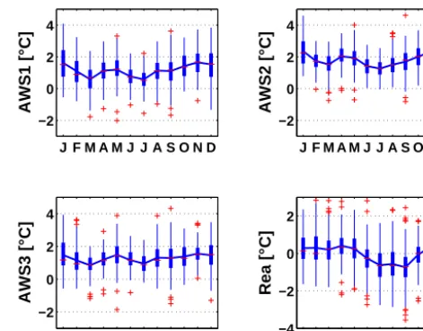
Figure 2. Monthly statistics of daily air temperature time se-ries at AWS1 (5050 m a.s.l.), AWS2 (4820 m a.s.l.), and AWS3 (4950 m a.s.l.), and of the a priori selected predictor rea-ens-air (as defined in the text). Shown are the means (blue solid line) and the medians (red dashes). The edges of the thick blue bars are the 25 and the 75 percentiles. The thin blue bars extend to the most ex-treme data not considered as outliers, and the red crosses are the outliers. All statistics are computed for period 1 (July 2006 to De-cember 2009).
Figure 2 shows statistics of AWS1, AWS2, and AWS3 daily mean air temperature for each calendar month, for pe-riod 1. The daily means are calculated from hourly samples measured at the AWSs. The daily mean air temperature val-ues are approximately normally distributed (not shown). The seasonal cycles in the data are small (<2◦C), showing
mul-tiple local minima and maxima throughout the year. This oc-currence of multiple maxima and minima, however, should not be overvalued as a climatology, because they are based on only 4 years of measurements. The interquartile ranges of the daily mean air temperature (blue bars in Fig. 2) amount to less than 2◦C in 50 % of all months, at all AWSs. The high-est within-month variabilities occur from December to Jan-uary, which points to El Niño–Southern Oscillation (ENSO) playing an important role in the region at this time of the year (e.g., Vuille et al., 2008b). Within-month variabilities are generally lower for the dry season months June to July. Also shown in Fig. 2 are statistics of the reanalysis data pre-dictor that will be referred to later.
2.3 Reanalysis data: the large-scale predictors
a fixed modeling system over the entire assimilation pe-riod, the reanalyses do not include data discontinuities due to changes in atmospheric model and assimilation techniques, as do the numerical weather prediction analyses. Thus, in terms of spatiotemporal completeness and consistency, re-analysis data are known to represent the most accurate es-timate of the past state of the atmosphere. However, a ma-jor source of uncertainty in the reanalysis data relates to changes in the observing system (e.g., Trenberth et al., 2001). Global reanalysis data are produced at five institutions world-wide: (i) the National Centers for Environmental Prediction, NCEP, (ii) the European Centre for Medium-Range Weather Forecasts, ECMWF, (iii) the Japan Meteorological Agency, JMA, (iv) the National Aeronautics and Space Administra-tion, NASA, and (v) the National Oceanic and Atmospheric Administration, NOAA (in cooperation with partner institu-tions not mentioned here for brevity).
To extend knowledge about the mountain glacier varia-tions to unobserved time periods or regions, more and more studies have relied on reanalysis data (e.g., Stahl et al., 2008; Kotlarski et al., 2010; Paul and Kotlarski, 2010; Marzeion et al., 2012; Mölg et al., 2012; van Pelt et al., 2012; Giesen and Oerlemans, 2013). For studies about the Cordillera Blanca and the South American Andes, the first-generation NCEP reanalyses have been a frequent choice (e.g., Garreaud et al., 2003; Vuille et al., 2008a, b; Hofer et al., 2010). Hofer et al. (2012), however, point out that the first-generation NCEP reanalyses show considerably weaker performance than several other reanalyses for the Cordillera Blanca, e.g., (i) the ERA-interim reanalyses by the ECMWF, (ii) the Mod-ern Era Retrospective-Analysis for Research and Applica-tions from NASA (MERRA), and (iii) the NCEP Climate Forecast System Reanalysis by the NCEP (CFSR).
3 SD model architecture
3.1 A priori predictor selection as a universal approach Generally, there are two ways of predictor selection: (1) a priori predictor selection (based on knowledge outside the data), and (2) data-based predictor selection (based on pre-ceding statistical analysis of the predictands). Most SD stud-ies more or less systematically use a combination of (1) and (2), by first pre-selecting a subset of potential predictors from an available pool based on process knowledge, and then choosing the definite, final predictors based on criteria de-rived from the data (e.g. Klein and Glahn, 1974; Wilby et al., 2002). Yet, data-based selection algorithms have encountered problems such as suboptimal skill of the SD model (e.g., Michaelsen, 1987; Stahl et al., 2008). Furthermore, the va-lidity of data-based selections is generally restricted to each specific site and to the data period of available observations, and generalizations thereof are usually impossible. In this study, we present, apply, and discuss systematic, a priori
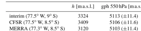
pre-Table 1. Specifications of the reanalysis data grid points applied as predictors: coordinates, surface heights (h), and mean geopotential heights (gph), with standard deviations in brackets, during the in-vestigation period (all values are in meters above see level).
h[m a.s.l.] gph 550 hPa[m a.s.l.]
interim (77.5◦W, 9◦S) 3324 5113 (±11.4) CFSR (77.5◦W, 8.5◦S) 3409 5106 (±11.6) MERRA (77.3◦W, 8.5◦S) 3120 5103 (±11.4)
dictor selection (thus, selection without looking at observa-tional data).
The proposed a priori selection strategy consists of three simple steps: (i) to relate the same physical predictor and pre-dictand variables; (ii) to consider the time series of this phys-ical variable at only one grid point, namely, the grid point lo-cated closest to the study site (in terms of latitude, longitude, and altitude); and (iii) to average these single grid point time series over several different, modern large-scale atmospheric data sets. This a priori predictor selection strategy reduces the five dimensions of the predictor space (here, latitude, longi-tude, altilongi-tude, physical variables, and large-scale data sets) to one dimension, without data analysis. This way, straight-forward application to different target variables and/or study regions is allowed for, without requiring subjective optimiza-tion. Limitations of this a priori predictor selection will be discussed in Sect. 5.
and CFSR. These three reanalysis data sets have already shown high skill with regard to daily air temperature varia-tions in the Cordillera Blanca (see Hofer et al., 2012). In this regard, their selection here is not independent from data anal-ysis. However, it is an intuitive choice, because all three re-analysis data sets have been produced very recently, are thus based on state-of-the art modeling systems, and are available at very high spatial resolutions. To sum up, in our study the a priori predictor consists of the average of three time series in total (of the three reanalysis models). This a priori pre-dictor (reanalysis-ensemble-air temperature) is abbreviated hereafter by rea-ens-air. Statistics of rea-ens-air computed over period 1 are shown in Fig. 2.
3.2 Preprocessing: accounting for seasonal periodicity If atmospheric time series are considerably shorter than 30 years and the climatological seasonal cycle is not known, the problem arises of how to strictly distinguish periodic, seasonal variations from aperiodic (or less periodic), day-to-day and inter-annual variability. Especially in statistical fore-casting, periodicity must be accounted for to avoid that the periodic, seasonal variations dominate the model fit. When long enough data series are available, the problem is gener-ally avoided by subtracting the climatological seasonal cycle from the time series (e.g., Madden, 1976). This way seasonal periodicity is removed from the time series, but not necessar-ily from the model error.
Here we assume that seasonal atmospheric periodicity leads to changing relationships between large- and local-scale atmospheric variables throughout the year. To consider the atmospheric seasonal cycle in SD models is important especially if the study site is located in the mountains. For example, local-scale atmospheric conditions can be affected by topographic shading that changes with the solar eleva-tion throughout the year. Due to the general discrepancies between the real topography and model topographies, how-ever, these effects are naturally not represented by the pre-dictors. Therefore, by using separate statistical predictor– predictand transfer functions for the different months of the year (or more generally also for different seasons, or Julian day numbers; e.g., Themeßl et al., 2011), seasonal periodicity is eliminated not only in the time series but also in the model error. Different transfer functions for the different calendar months are used often also in SD models that rely on stochas-tic weather generators (e.g., Wilby and Dawson, 2007).
In practice in this study, the predictor–predictand pairs are divided into 12 separate time series, one for each calendar month. The number of observations in each time series con-sequently amounts to approximatelyn=N/12, whereN is the length of the entire time series. Hence, all steps of model training and validation (described in the next section) are re-peated individually for each calendar month’s time series, ym(t )(ym(t )consists of the concatenated daily mean time series of January 2007, January 2008, January 2009, etc.).
For simplicity in the following sections, we use the symbol
y(t )for each of the 12 calendar months’ time series, omitting
the index m for months.
3.3 SD model training and validation
The simplest way to relate an a priori predictor to a target variable is a simple linear regression model. It applies
y(t )=α1+α2·x(t )+(t ). (1)
In Eq. (1),y(t )is the local-scale target variable (the predic-tand) that varies with timet.x(t )is the predictor time series (here, a single time series).α1andα2are the least-squares re-gression parameters (intercept and slope).α1andα2are esti-mated by minimizing the model error,(t ), which is assumed to follow a Gaussian distribution with zero mean. Note that least-squares regression does not account for the time order-ing in the data series, and the parameters in Eq. (1) are there-fore not affected by the use of discontinuous, concatenated (month-separated) time series. Note further that linear least-squares regression is usually problematic for target variables which strongly deviate from a Gaussian distribution. More precisely, for non-Gaussian variables the normality assump-tion of (t ) is usually violated. Potential modifications of the SD model presented here for non-Gaussian target vari-ables are mentioned in Sect. 5. The analytical solutions for the least-squares parametersα1andα2yield:
α1=y−α2·x,
α2=r·Rσ, (2)
withx andybeing the temporal means ofx(t )andy(t ), re-spectively, and
Rσ =
σ (y)
σ (x),
r= σ (x, y)
σ (x)·σ (y). (3)
In Eq. (3),σ (y) is the temporal standard deviation ofy(t ),
σ (x)is the temporal standard deviation ofx(t ), andσ (x, y)
is the sample covariance ofy(t ) andx(t ).r is the Pearson correlation coefficient (e.g., Von Storch and Zwiers, 2001).
ˆ
y(t )are the predictions from the SD model, defined as
fol-lows: ˆ
y(t )=α1+α2·x(t )=y(t )−(t ). (4)
The SD model is trained and validated based on a mod-ification of leave-one-out cross-validation described in the following. For each calendar month’s time series, the least-squares parameter estimation is repeatedntimes, withn be-ing the number of observations of each calendar month’s time series. Each time,nlo observations are excluded from the model fit (the left-out observations), with
τρ∼=0is the temporal lag, for which the autocorrelation
func-tion of each (concatenated) calendar month’s time series
(y(t )is within the 95 % confidence interval of the
autocor-relation for Gaussian white noise. The 95 % confidence in-terval is approximated with 2/n1/2.τρ∼=0 is also known as decorrelation time (e.g., Von Storch and Zwiers, 2001). In each cross-validation repetition, nT=n−nlodata pairs are used for the least-squares parameter estimation (the index T denotes training). We use the notation yT for thenT train-ing observations that slightly differ in each turn of the cross-validation, andyˆTfor the SD model estimated based onyT. The central of thenlowithheld observations can then be con-sidered as independent from the calibration process, and is used to estimate the model test error,V(t ). By repeating the above-described procedurentimes, each observation iny(t ) is used once as independent observation for estimatingV(t ):
V(t )=y(t )− ˆyV(t ). (6)
By contrast to(t ),V(t )is not involved in the model train-ing process, and is thus more useful for the determination of the model skill. Above,yˆV(t )is the SD model estimated indi-vidually for each time steptbased on all observations despite
[y(t−τρ∼=0). . .y(t+τρ∼=0)]. This way,ndifferent estimates of
the SD model parameters in Eq. (2) result, being based onn (slightly) varying sub-samples ofy(t ). The resulting variance of the SD model parameters is a measure of the stability of the model parameters (e.g., with regard to influential outliers, see Michaelsen, 1987). The average of the SD model param-eters is used to calculate the final SD model predictions,y(t )ˆ , for each calendar month. The complete SD model time series is then obtained by putting together in chronological order the 12 calendar month’s SD models.
3.4 Skill estimation and significance analysis
When the cross-validation process is completed, the skill score (SS) can be calculated as follows (e.g. Wilks, 2006): SS=1− mse
mser
, (7)
with mse=1
n·
X
V2(t ). (8)
mserin Eq. (7) is the mean of squared errors of the reference model yˆr:=yT, withyT(t )being the temporal mean ofyT,
andr(t )=y(t )− ˆyr:
mser= 1
n·
X
2r(t ). (9)
Note that SS is a relative accuracy measure, which can be decomposed into the squared Pearson product-moment cor-relation between the observations and the validation forecasts
ryyˆ:=r y(t ),yˆV(t ), deflated by two penalty terms, as
fol-lows (e.g., Murphy, 1988; Wilks, 2006):
SS=ry2yˆ− [ryyˆ−
σ (yˆV)
σ (y)
i2
−hy¯ˆV− ¯y σ (y)
i2
. (10)
Above,σ (y)andσ (yˆV)are the temporal standard deviations
ofy(t )andyˆV(t ), andy¯ andy¯ˆV are the temporal means of
y(t )andyˆV(t ). The second term in Eq. (10) is a measure of
reliability, or conditional bias, and the third term in Eq. (10) is the square of the unconditional bias standardized byσ (y). For least-squares regression, the second and third terms in Eq. (10) are usually zero. However, because for each time step t, the least-squares model training for yˆV(t ) is inde-pendent from y(t ) (since the training sample used to esti-mateyˆV(t )does not includey(t )nor nearby, correlated data points), the terms will usually differ from zero.
Below, we show an application of the SD model frame-work for short measurement series (about 3- to 7-year mea-surements, as introduced in Sect. 2). In order to give an ob-jective quantification of whether the available time series are long enough for the SD model and skill assessment to be re-liable (and useful), we determine if SS is significantly larger than 0 as follows. Because of Eq. (7), SS>0 implies that mser−mse>0. Because of the linearity of the mean, this further impliesds >0, withds(t ):=r2(t )−V2(t ), and· denoting the mean over allntime steps. To estimate the sam-pling distribution of the mean of the squared error differences ds, we use moving block bootstrap. Moving block bootstrap is a variant of bootstrap that preserves the temporal autocor-relation structure of a time series. It works in the same way as ordinary bootstrap (e.g., Wilks, 2006), but instead of re-sampling fromnindividual (independent) observations, the resampling is based on blocks of observations of lengthL. Here, we useLas approximated for first-order autoregres-sive processes (AR(1)by Wilks (1997), based on the im-plicit equation
L=(n−L+1)(2/3)(1−neff/n), (11)
with
neff≈n
1−ρ1 1+ρ1
. (12)
2006/3/1−2 2007/3/1 2008/3/1 2009/3/1 2010/3/1 2011/3/1 0
2 4
March time series [days]
AWS1 air t [°C]
2006/7/1−2 2007/7/1 2008/7/1 2009/7/1 2010/7/1 2011/7/1
0 2 4
July time series [days]
AWS1 air t [°C]
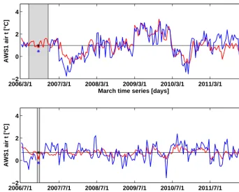
Figure 3. Example of the SD model skill estimation based on cross-validation as described in Sects. 3.3 and 4.1, for AWS1 predictands and the rea-ens-air predictor in March (top) and July (bottom):yT(t )(blue line),y(t )ˆ based onyT(t )(red line), theyˆr (black line),y(t ), the observation considered independent from the model process (blue star), the corresponding value ofyˆV(t )(red star), and ofyˆr (black star). The gray shaded area highlights the observations left out in the model calibration process (for illustration here, at cross-validation step 15). Note that the gray bar changes its position at each cross-validation step (as described in the text).
observation time series is stepwise reduced, and the SD mod-eling procedure and the skill assessment are repeated, until SS is no longer found to be significant. This way, 12 num-bers are obtained that represent the minimum number of ob-servations required in each calendar month to construct a SD model with statistically significant skill.
4 Results and discussion
4.1 Demonstration of the model training and validation procedure
Figure 3 provides a comprehensible example of the skill esti-mation procedure described above. The two plots show daily air temperature time series (yTof the months March (top) and July (bottom) at AWS1 (blue line). The example shows the SD model building and error estimation in an individ-ual repetition of the least-squares regression procedure in the frame of the modified leave-one-out cross-validation. The gray bar indicates thenloobservations left out in the model calibration. Note that for each of the n parameter estima-tion repetiestima-tions, the gray bar is shifted one observaestima-tion to the right. The number of observations left out is determined by the cross-validation parameterτρ∼=0. The values ofτρ∼=0
are 11 in March, and 3 in July. This means that, e.g., in the March time series an observation is considered independent from an other observation only if there is a shift of at least 11 time steps (in this case, days) between the two observa-tions. Thus, for the March time series the gray bar includes 11·2+1=23 left-out observations. The red line isyˆT. The errorV(t )of Eq. (6) is then estimated as the difference be-tween the central observationy(t )(blue star in the gray bar in Fig. 3), and the model value at this time stepyˆV(t )(red star in the gray bar in Fig. 3).yˆr used to calculatemserin Eq. (9) is the black star in Fig. 3 (identical with the black line), calculated as the mean ofyT, the observations used in the model training. Cross-validation is repeated until each observationy(t )is used once to determine the model error. This way independence between the observations used in the model training and the validation process is guaranteed, and at the same time all observations can be used to determine the final SD model.
4.2 SD model parameters
0 0.2 0.4 0.6 0.8
r
J F M A M J J A S O N D
0 0.5 1 1.5
R σ
Figure 4. Boxplots of the ESD model parameters: medians (dots) of the downscaling model parametersr(top) andRσ(bottom) esti-mated by cross-validation with AWS1 air temperature as the predic-tands and rea-ens-air as the predictor, for all calendar months. The edges of the boxes are the 25th and the 75th percentiles. The dashes extend to the most extreme data not considered as outliers.
relationship (see Eq. 2). Both r andRσ show a remarkably high inter-monthly variability. Also shown in Fig. 4 are the uncertainties ofrandRσ (the edges of the boxes indicate the 25 and 50 percentiles of the regression parameters estimated in each repetition of the least-squares procedure of the cross-validation). Values of r are higher than 0.6 for the months January to May (wet season in the Cordillera Blanca), and in September. For the remaining months (June to August, November and December), values ofr are between 0.4 and 0.6. The largest sampling uncertainties ofr are evident for the months February to April.Rσ throughout the year varies from approximately 0.9 to 1.4. Values of Rσ close to one (e.g., for the calendar months May to August) imply that the standard deviation of the predictand is similar to the stan-dard deviation of the predictor. Values ofRσ larger than one (e.g., for December) imply that the standard deviation of the predictand is larger than the standard deviation of the pre-dictor (see Eq. 3). To sum up, while values of r indicate a strong predictor–predictand relation, the high variations of the downscaling parameters throughout the year clearly show the importance of using distinct models for each calendar month.
Figure 5 shows values of the cross-validation parameter τρ∼=0 of the 12 calendar months for data from AWS1 (red
circles). As defined in Sect. 3.3, τρ∼=0 can be interpreted
as the temporal lag in days, for which the daily mean air temperature values can be assumed to be independent. Val-ues ofτρ∼=0vary between 3 (weak persistence) and 20 days (strong persistence) for the different calendar months. For the months January to April, values of τρ∼=0 are consider-ably higher (13, 11, 11 and 20 days, respectively) than for the remaining months. These higher values ofτρ∼=0are
prob-J F M A M J J A S O N D
0 100 200
n min
[days]
J F M A M J J A S O N D 0
10 20
τ ρ=0
[days]
Figure 5. The black circles show the minimum number of AWS1 air temperature observations required for each calendar month’s model to obtain statistically significant skill (nmin, based on rea-ens-air, as described in the text). The red circles (right axes) show the decor-relation time (τρ∼=0), for each month’s daily air temperature time series recorded at AWS1.
ably due to high intra-seasonal variations of humidity and rainfall in those months that also affect the air temperature variations. More specifically, intra-seasonal variability in the tropical Andes is characterized by rainy episodes in terms of wet-day sequences followed by dry-day sequences, and are associated to variances of air temperature (Garreaud et al., 2003). Overall in the tropics, such synoptic episodes typi-cally range from 30 to 60 days (with the basic mechanism known as the Madden–Julian Oscillation, MJO; Madden and Julian, 1994). For the Bolivian Altiplano (located nearby the Cordillera Blanca), however, Garreaud et al. (2003) reported shorter synoptic periods of approximately 15 days in length. Please note that by examiningτρ∼=0of the month-separated and concatenated time series, it is not possible to identify the full length of the MJO cycles. Small values ofτρ∼=0 es-pecially for the austral winter months indicate small inter-annual variability. In other words, there are no important dif-ferences amongst the different years of the respective austral winter months. In fact, ENSO, the most important source of inter-annual variability in the region, has its strongest and most widespread impacts during austral summer.
4.3 Skill assessment
J F M A M J J A S O N D 0
0.2 0.4 0.6 0.8 1
SS
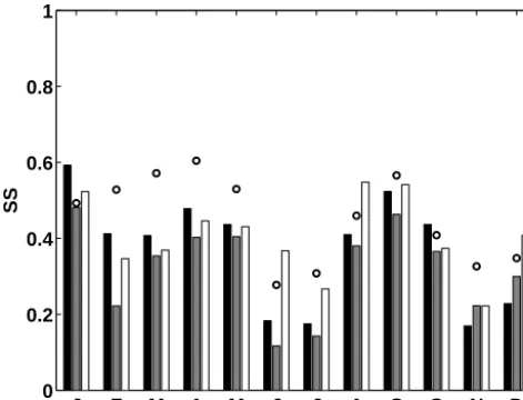
Figure 6. Values of SS for AWS1 (black), AWS2 (gray), and AWS3 (white) for the predictor rea-ens-air for period 1. The open circles show the respective values of SS at AWS1 for its entire data period (period 2).
months February to April. The high values of SS in the wet season imply that the largest portion of day-to-day variabil-ity of AWS1 air temperature can be explained by rea-ens-air. This indicates spatially very homogenous air temperature fluctuations for these months of the year. In fact, Garreaud et al. (2003) reported spatially very coherent intra-seasonal weather patterns for the nearby Bolivian Altiplano, and also the MJO is known to act on large spatial scales (with local wavelengths of 1.2−2×10³km). By contrast in the core dry season, values of SS for rea-ens-air reach only half of the wet season values. A possible explanation is that variability in the dry season might be governed by processes that act more locally (e.g., processes that are triggered by the com-plex topography). We further hypothesize that the generally weaker synoptic forcing during the dry season impacts the local-scale variability in a more subtle way, which is not re-solved with the single linear predictor rea-ens-air. In Fig. 3 (lower panel), the SD model predictions for daily air temper-ature in the dry season month July show only minor variance. Also the variability in the observational time series is evi-dently smaller for July than for the wet season month March (upper panel in Fig. 3). Nevertheless, the underestimation of observed variance is smaller for the wet season month March, indicating higher co-variability between the predictor and predictand time series. The values of SS based on period 1 show a similar seasonal pattern for all AWSs (see Fig. 6). However, the seasonal patterns of SS for AWS1 differ among the two periods, period 1 versus period 2. For period 1, the values of SS are generally lower than for period 2. This is an expected result, because increasing the database for the model training (from period 1 to period 2) allows for a more accurate estimation of the model parameters (since nT in-creases), and consequently the values of SS are higher. With
Table 2. Values of SS andr2for the three assessed AWSs, averaged over all months of the year, estimated using the entire measuring pe-riods from each AWS, and in brackets the respective values based on period 1 (only for AWS1 and AWS2, because the entire measur-ing period of AWS3 is per definition equal to period 1).
AWS1 AWS2 AWS3
r2 0.47 (0.4) 0.5 (0.38) 0.48 SS 0.45 (0.37) 0.48 (0.32) 0.4
Table 3. List of predictors (and their abbreviations) assessed in Sect. 4.4.
shm specific humidity at 550 hPa gph geopotential height at 550 hPa
air air temperature at 550 hPa uwn zonal wind speed at 550 hPa vwn meridional wind speed at 550 hPa
spr surface pressure
vor potential vorticity at 550 hPa t2m air temperature at 2 m a.s.l. wwn vertical wind speed
further increase of available training data, the dependence of SS on the length of the training series is expected to decrease (e.g., Hastie et al., 2001).
The significance analysis reveals that values of SS in Fig. 6 are significant at the 5 % test level, for all calendar months and AWSs. Figure 5 showsnmin, at the example of data from AWS1, for each calendar month.nminis related to SS, in a way that for higher values of SS, nmin tends to be lower. nmin largely varies from a minimum value of 33 (and 36) for the calendar months May (and March), to 136 for the calendar months July. Since the AWS1 time series includes more than 120 to 150 observations per calendar month for period 1, and 210 observations for period 2,nminis exceeded for each calendar month, however, only by a small margin for July and November for period 1. Values of SS andr2 av-eraged over all calendar months are shown in Table 2, for the different AWSs. The values are shown for the measuring pe-riods of each AWS (thus period 1 for AWS3), and for AWS1 and AWS2 additionally for period 1. On average, SS is high-est at AWS2 (mean SS=0.48) and lowest at AWS3 (mean SS=0.4). As discussed above for AWS1, values of SS are considerably lower for the shorter, common time period (pe-riod 1), for which AWS2 shows even the lowest values of SS. Table 2 further shows that values ofr2overestimate the skill, compared to SS based on cross-validation, with up to 0.08 higher values (see AWS3).
4.4 Towards automated predictor selection
J F M A M J J A S O N D 0
0.2 0.4 0.6 0.8 1
SS
gph air t2m
Figure 7. Values of SS for each month (here for AWS1), and the three predictors of those assessed in Sect. 4.4, which showed signif-icant results.
the performance of various predictor variables, to demon-strate how the skill assessment presented here can be used for data-based predictor selection. Table 3 gives a list of all abbreviations of the nine assessed predictor variables: shm, gph, air, uwn, vwn, spr, vor, t2m, and wwn. In this sec-tion, all predictor variables are considered from the ERA-interim. We do not consider the multiple reanalysis ensem-bles as above, because (i) not all variaensem-bles are available by all reanalyses as analysis values, and (ii) there are inhomo-geneities in the CFSR variables spr and wwn between data prior and after December 2010. These inhomogeneities are due to changes in the model configurations from CFSR avail-able until December 2010, to the subsequently operationally available CFSV2. Furthermore, ERA-interim have shown the highest skill for air temperature predictands in the Cordillera Blanca out of all individual global reanalyses, and compa-rably high skill as the ensemble from multiple reanalyses (Hofer et al., 2012). However, unlike multiple reanalysis en-sembles, individual reanalyses need to be considered at their optimum scale, in order to eliminate numerical noise related to single grid point data (Hofer et al., 2012). Here, we adopt the optimum scale of the ERA-interim determined by Hofer et al. (2012) for air temperature in the Cordillera Blanca, which is relatively small: four times four grid points centered horizontally around the study site.
The results of the skill assessment reveal significant skill for only three of the assessed predictor variables: air, t2m, and gph. Values of SS of these variables are shown in Fig. 7 for each calendar month, and AWS1 data. For all other vari-ables listed in Table 3, the values of SS are non-significantly different from zero; moreover, t2m clearly shows lower val-ues of SS than air in all months. Thus, the reanalysis vari-ables that are less affected by the model surface actually emerge as the better predictors for near-surface predictand
1 2 3 4 5 6
0 0.2 0.4 0.6 0.8 1
timescale [days]
SS
J F M A M J J A S O N D
Figure 8. Values of SS for all assessed timescales (daily averages to 6-daily averages) and the 12 calendar months (colors of the bars, January to December), for which SS is found to be significant at each timescale. Shown here is the example of the predictor rea-ens-air for AWS1 daily rea-ens-air temperature as target variable. The values of SS are divided by 12 (the number of calendar months), such that the sum of the bars is equivalent to the average SS, at each of the timescales.
hourly daily
0 0.1 0.2 0.3 0.4 0.5 0.6 0.7 0.8
r
2
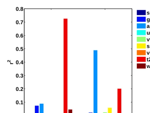
shm gph air uwn vwn spr vor t2m wwn
Figure 9.r2for 6-hourly and daily (all-month) time series of AWS1 air temperature and all predictors assessed in Sect. 4.4.
(2) the a priori choice of relating the same physical variables in the predictor–predictand transfer function is supported by the data-based analysis; and (3) even if values of SS show a distinct seasonal cycle, the same predictor (i.e., air) shows the highest skill throughout the year.
4.5 Application of the SD model at varying timescales
In this section, we systematically investigate the skill of the reanalysis predictors for temporal resolutions beyond the daily timescale. We repeat the modeling procedure as intro-duced in Sect. 3, for the AWS1 time series aggregated from daily to 2-daily, 3-daily, 4-daily, 5-daily, and 6-daily means. 6-daily means represent the lowest temporal resolution, at which statistically significant skill is obtained for all calen-dar months’ models in the application example of our study. In this experiment, we assess each timescale based on a fixed number of time steps (nexp), in order to allow for a com-parison of SS amongst the different timescales.nexpis deter-mined by (i) the lowest temporal resolution considered (here, 6-daily means), and (ii) the sample size of each month’s time series. More specifically, if a calendar month’s time series consists of 144 daily means, it can be aggregated to a series of 24 6-daily means, and thus nexp is fixed to 24. In order to avoid arbitrary sub-sampling ofnexp observations for the higher time resolutions (daily to 5-daily, of which more than nexptime steps are available for the underlying time series), we perform a systematic sub-sampling in terms of moving blocks ofnexpconsecutive observations, until each observa-tion has been considered the same number of times (at each timescale, and for each calendar month). The modeling pro-cedure is then repeated for each sub-sample, and the results are averaged over all repetitions. Figure 8 shows values of SS for different temporal resolutions, and the 12 calendar months of AWS1 data. The values of SS are divided by 12, such that their sum corresponds to the average skill for each timescale (total length of each colored bar in Fig. 8). Note that the values of SS shown here are lower than the values of SS found in Fig. 6, becausenexpis smaller thannfor all timescales. SS shows an increase for longer averaging inter-vals. The increase of the average skill is most notable from the daily to the 2-daily timescale, whereas for the 4- to 6-daily timescale, only very small differences are evident.
Finally, we show a simple analysis to demonstrate the ef-fects of periodicity (here, diurnal) for regression analysis based solely on r2 (an often applied criterium for predic-tor selection). Figure 9 shows values ofr2between 6-hourly (all-month) time series of AWS1 air temperature, and the predictors assessed in Sect. 4.4: shm, gph, air, uwn, vwn, spr, vor, t2m, and wwn. The same analysis is shown at a daily timescale, where the diurnal cycle is eliminated by av-eraging the 6-hourly data to daily means. Values of r2for the 6-hourly data (left hand side in Fig. 9) clearly suggest t2m as the best predictor, showing a relatively high corre-lation (r2>0.7). All other predictors (including air) show
only minor correlation to the predictand (r2<0.1). This pat-tern significantly changes at the daily time resolution (right hand side in Fig. 9): now the predictor air shows the high-est correlation (r2 is almost 0.5), but t2m shows only very small correlations (r2=0.2 – yet still higher than all other assessed predictors). In the diurnal analysis, t2m appears as important predictor only because of its pronounced diurnal variations which explain the largest portion of variability also in the predictand data. However, this is achieved easily with a constant diurnal cycle. For example, the correlation between the hourly air temperature series, and a time series composed by consecutive constant diurnal cycles is r2=0.7. There-fore, predictor selection that does not account for diurnal (or other) periodicity is not meaningful. Even though this is by no means innovative in statistics, the issue of periodicity is not accounted for appropriately in numerous studies in the cryospheric sciences.
5 Limitations and outlook
interactions expressed by the governing atmospheric equa-tions. However, the disadvantage of LAMs, compared to SD, is their high computational expense.
The SD model presented here consists of 12 different predictor–predictand transfer functions, for the 12 calendar months of the year. Even though these transfer functions are tested based on independent data (using cross-validation), there is no guarantee that the transfer functions remain sta-tionary beyond the observation period. Here we enter into the problem of the stationarity assumption underlying SD mod-els, e.g., the validity of the transfer functions for different climatic periods, or for different phases of ENSO. While as-sessing the validity of the SD stationarity assumption goes beyond the scope of our study, we like to point out that a pri-ori selections are usually based on assumptions that are inde-pendent from the observation period, while data-based selec-tions are strongly linked to the observation period. Therefore, assuming temporal stationarity is more problematic for data-based selections than for a priori selections. A systematic in-vestigation of the consistency of SD models for precipitation over century to millennium timescales is given in the work by Frías et al. (2006).
Because for leave-one-out cross-validation each training data set contains almost as many data as the original time series, it is useful especially in the case of short observa-tional time series. For sufficiently long time series, a fre-quently applied, computationally cheaper alternative is k -fold cross-validation (withkbeing typically 5 or 10). Here, sufficiently long means long enough such that the skill of the SD model no longer depends on the length of the data series (see also the issue of bias-variance trade off fork-fold cross-validation, Hastie et al., 2001). In technical terms, leave-one-out cross-validation is similar to (and therefore often mistak-enly referred to as) the jackknife resampling technique. The jackknife, however, is generally used in a different context: i.e., for non-parametric estimation of the bias and/or stan-dard deviation of a sampling distribution from data in a sin-gle sample (e.g., Wilks, 2006). As not shown in this study, cross-validation is powerful especially for multiple regres-sion problems. Then,x(t )in Eq. (1) has multiple columns, x∈R(n×p) withnrepresenting the number of observations in the time series, and p the number of predictors inx. In fact, SS based on cross-validation is a powerful statistic to detect over-fitting in the case of multiple predictors. More precisely, in the case of over-fitting, SS as defined in Eqs. (7) and (10) will be equal or smaller than zero, and the sig-nificance analysis presented here will reveal no significant skill. More detailed overviews about cross-validating mul-tiple predictor-regressions to protect against over-fitting are given in the statistical textbooks by Hastie et al. (2001), and Wilks (2006).
The significance testing of SS in this study is a recom-mended version of hypothesis testing for forecast verifica-tion statistics (Mason, 2008), which does not involve the bootstrap estimation of the distribution of the null
hypoth-esis (by contrast to classical statistical hypothhypoth-esis testing). In our study, the null hypothesis that SS is equal or smaller than zero is evaluated by examining its unusualness with respect to the 95 % bootstrap confidence intervals of SS (e.g., Wilks, 2006). Further note that the moving block bootstrap applied in our study is based on the condition that the squared error differences ds(t )underly an AR(1) process. In the applica-tion example of our study, the ds(t )time series support the AR(1) assumption; however, this is not necessarily the case. Therefore, it is important to assess the autocorrelation func-tion of ds(t )prior to the application of the moving block bootstrap. Adaptations of the block lengthLfor AR(2) pro-cesses and for autoregressive moving average propro-cesses are proposed in the work of Wilks (1997).
Finally, we would like to add a few notes on the extension of the SD model for Gaussian target variables. For non-Gaussian target variables, the application of ordinary least-squares regression in Eq. (1) is often problematic, because then the normality assumption of the model error is usually violated. In this case, there are several possibilities to ex-tend the SD modeling procedure presented here. A simple way to include non-Gaussian target variables is to prepro-cess the target variable prior to the input in the regression procedurey0(t )=f y(t ), such thaty0(t )follows a normal distribution (e.g., by means of power transformations, Wilks, 2006). More complex, yet flexible modifications of the mod-eling procedure for non-Gaussian targets include the replace-ment of the least-squares linear regression procedure applied here (Eq. 1 to Eq. 3) by generalized linear modeling. Fur-thermore, when nonlinear predictor–predictand relationships are evident from the underlying physics, nonlinear regres-sion may replace the linear regresregres-sion. In the case of gener-alized linear models and nonlinear regression, ordinary least-squares regression is usually replaced by iterative fitting pro-cedures, or maximum likelihood methods (see Wilks, 2006). After the replacement of Eq. (1) with Eq. (3), with the ap-propriate model representation for non-Gaussian targets, the skill estimation of the SD model for short, autocorrelated ob-servation time series (Eq. 7 to Eq. 12) can be equally applied as described above (not shown).
6 Summary and conclusions
models for the different months of the year. The presented skill estimation is based on a modification of leave-one-out cross-validation combined with moving block bootstrap to appropriately account for autocorrelation in the observational data, and in the SD model error.
We have shown an application of the SD model with re-analysis data as the predictors, and daily mean air temper-ature measured at three high-altitude sites in the glaciated Cordillera Blanca (Peru) as the target variables. First, the skill of the a priori predictor rea-ens-air is assessed. High seasonality of statistical data properties (e.g. persistence) and SD model parameters emphasize the importance of using dif-ferent models for difdif-ferent calendar months. The SD model skill shows high seasonality as well, with generally higher skill in the wet season, and lower skill in the dry season. Whereas differences in the SD model skill for the different AWSs are small, the skill increases with increasing observa-tion availability. The skill is shown to be significant at a 5 % test level, if at least 33 to 140 daily observations are avail-able per calendar month. In particular, the calendar months for which the SD model shows low skill require consid-erably more data for the SD model to be significant (e.g., July). The a priori predictor air temperature from the pres-sure level of the study sites (air) shows clearly higher skill than other skillful predictors, such as air temperature at two meters above the model surface (t2m), or geopotential height of the pressure level of the study sites (gph). Six further as-sessed reanalyses predictors show no significant skill. Inves-tigating a model’s skill without taking account of natural pe-riodicity leads to spuriously high performance of t2m at a diurnal timescale, compared to air, due to the pronounced diurnal cycle of t2m. If the same number of time steps is used to train the SD model at different temporal resolutions (i.e., from daily to 6-daily averages), the skill averaged over all months increases considerably from daily to 2-daily time steps, with only minor increases for further increasing av-eraging intervals. The entire SD modeling framework, pre-sented here for high-altitude air temperature in the tropical Cordillera Blanca, can be transferred to a variety of applica-tions. The a priori selection strategy, the data preprocessing, and the SD model training and validation are designed to be applicable to all Gaussian target variables, at mountainous sites in various climatic and geo-environmental settings.
Acknowledgements. This study was funded by the Austrian Science Fund (FWF): P22106-N21. Marlis Hofer was supported through a research grant of the University of Innsbruck. Thomas Mölg was supported by the Alexander von Humboldt Foundation. ERA-interim data are provided by the ECMWF. MERRA are disseminated by the GMAO and the Goddard Earth Sciences Data and Information Services Center (GES DISC). CFSR are obtained by the Research Data Archive (RDA) which is maintained by the Computational and Information Systems Laboratory (CISL) at the National Center for Atmospheric Research (NCAR). We greatly acknowledge several anonymous referees that contributed
considerably to improving the article.
Edited by: W. Hazeleger
References
Ames, A.: A documentation of glacier tongue variations and lake developement in the Cordillera Blanca, Peru, Zeitung für Gletscherkunde und Glazialgeologie, 34, 1–36, 1998.
Bair, E., Hastie, T., and Tibshirani, R.: Prediction by Super-vised Principal Components, J. Am. Stat. Assoc., 101, 119–137, doi:10.1198/016214505000000628, 2006.
Benestad, R., Førland, E. J., and Hanssen-Bauer, I.: Empirically downscaling temperature scenarios for Svalbard, Atmos. Sci. Lett., 3, 71–93, doi:10.1006/asle.2002.0050, 2002.
Benestad, R. E., Hanssen-Bauer, I., and Deliang, C.: Empirical-statistical downscaling, World Scientific, Singapore, 2008. Carey, M.: Living and dying with glaciers: people’s historical
vul-nerability to avalanches and outburst floods in Peru, Global Planet. Change, 47, 122–134, 2005.
Carey, M.: In the Shadow of Melting Glaciers. Climate Change and Andean Society, Oxford University Press, 2010.
Cavazos, T. and Hewitson, B. C.: Performance of NCEP-NCAR re-analysis variables in statistical downscaling of daily precipita-tion, Climate Res., 28, 95–107, 2005.
Christensen, J. H., Hewitson, B., Busuioc, A., Chen, A., Gao, X., Held, I., Jones, R., Kolli, R. K., Kwon, W.-T., Laprise, R., Mag-aña Rueda, V., Mearns, L., Menéndez, C. G., Räisänen, J., Rinke, A., Sarr, A., and Whetton, P.: Regional Climate Projections, in: Climate Change 2007: The Physical Science Basis, Contribution of Working Group I to the Fourth Assessment Report of the In-tergovernmental Panel on Climate Change, edited by: Solomon, S., Qin, D., Manning, M., Chen, Z., Marquis, M., Averyt, K. B., Tignor, M., and Miller, H. L., Cambridge University Press, Cam-bridge, United Kingdom and New York, NY, USA, 2007. Frías, M. D., Zorita, E., Fernández, J., and Rodríguez-Puebla, C.:
Testing statistical downscaling methods in simulated climates, Geophys. Res. Lett., 33, L19807, doi:10.1029/2006GL027453, 2006.
Garreaud, R., Vuille, M., and Clement, A.: The climate of the Al-tiplano: observed current conditions and mechanisms of past changes, Palaeogeography, Palaeoclimatology, Palaeoecology, 194, 5–22, doi:10.1016/S0031-0182(03)00269-4, 2003. Georges, C.: Ventilated and unventilated air temperature
measure-ments for glacier-climate studies on a tropical high mountain site, J. Geophys. Res., 107, 2156–2202, doi:10.1029/2002JD002503, 2002.
Georges, C.: 20th-century glacier fluctuations in the tropical Cordillera Blanca, Peru, Arctic, Antarctic, Alpine Res., 36, 100– 107, 2004.
Georges, C.: Recent Glacier Fluctuations in the Tropical Cordillera Blanca and Aspects of the Climate Forcing, Ph.D. thesis, Leopold-Franzens University Innsbruck, Innsbruck, Austria, 2005.
Giorgi, F. and Bates, G. T.: The climatological skill of a regional model over complex terrain, Mon. Weather Rev., 117, 2325–2347, doi:10.1175/1520-0493(1989)117<2325:TCSOAR>2.0.CO;2, 1989.
Grotch, S. L. and MacCracken, M. C.: The use of global climate models to predict regional climatic change, J. Climate, 4, 286– 303, 1991.
Hastie, T., Tibshirani, R., and Friedman, J.: The elements of statis-tical learning: data mining, inference, and prediction, Springer series in statistics, Springer, New York, 1 edn., 2001.
Hessami, M., P. G., Ouarda, T. B. M. J., and St-Hilaire, A.: Auto-mated regression-based statistical downscaling tool, J. Environ. Model. Softw., 23, 813–834, doi:10.1016/j.envsoft.2007.10.004, 2008.
Hill, G. E.: Grid Telescoping in Numerical Weather Pre-diction, J. Appl. Meteorol., 7, 29–38, doi:10.1175/1520-0450(1968)007<0029:GTINWP>2.0.CO;2, 1968.
Hofer, M., Mölg, T., Marzeion, B., and Kaser, G.: Empirical-statistical downscaling of reanalysis data to high-resolution air temperature and specific humidity above a glacier surface (Cordillera Blanca, Peru), J. Geophys. Res.-Atmos., 115, 2156– 2202, doi:10.1029/2009JD012556, 2010.
Hofer, M., Marzeion, B., and Mölg, T.: Comparing the skill of dif-ferent reanalyses and their ensembles as predictors for daily air temperature on a glaciated mountain (Peru), Clim. Dynam., 39, 1969–1980, doi:10.1007/s00382-012-1501-2, 2012.
Huth, R.: Sensitivity of local daily temperature change estimates to the selection of downscaling models and predictors, J. Climate, 17, doi:10.1175/1520-0442(2004)017<0640:SOLDTC>2.0.CO;2, 2004.
Juen, I.: Glacier mass balance and runoff in the Cordillera Blanca, Peru, PhD thesis, University of Innsbruck, 2006.
Juen, I., Georges, C., and Kaser, G.: Modelling observed and future runoff from a glacierized tropical catchment (Cordillera Blanca, Peru), Global Planet. Change, 59, 37–48, 2007.
Kaser, G. and Osmaston, H.: Tropical Glaciers, International Hy-drology Series, Cambridge University Press, Cambridge, UK, 2002.
Kaser, G., Juen, I., Georges, C., Gomez, J., and Tamayo, W.: The impact of glaciers on the runoff and the reconstruction of mass balance history from hydrological data in the tropical Cordillera Blanca, Peru, J. Hydrol., 282, 130–144, 2003.
Kaser, G., Grosshauser, M., and Marzeion, B.: The contribution potential of glaciers to water availability in different climate regimes, Proc. Natl. Acad. Sci. USA, 107, 20223–20227, 2010. Kidson, J. W. and Thompson, C. S.: A comparison of statistical
and model-based downscaling techniques for estimating local climate variations, J. Climate, 11, 735–753, doi:10.1175/1520-0442(1998)011<0735:ACOSAM>2.0.CO;2, 1998.
Klein, W. H. and Glahn, H. R.: Forecasting local weather by means of model output statistics, B. Am. Meteorol. Soc., 55, 1217– 1227, 1974.
Klein, W. H., Lewis, B. M., and Enger, I.: Objective prediction of five-day mean temperature during win-ter, J. Meteorol., 16, 672–682, doi:10.1175/1520-0469(1959)016<0672:OPOFDM>2.0.CO;2, 1959.
Kotlarski, S., Paul, F., and Jacob, D.: Forcing a Distributed Glacier Mass Balance Model with the Regional Climate Model REMO.
Part I: Climate Model Evaluation, J. Climate, 23, 1589–1606, doi:10.1175/2009JCLI2711.1, 2010.
Madden, R. A.: Estimates of the Natural Variability of Time-Averaged Sea-Level Pressure, Mon. Weather Rev., 104, 942–952, doi:10.1175/1520-0493(1976)104<0942:EOTNVO>2.0.CO;2, 1976.
Madden, R. A. and Julian, P. R.: Observations of the 40 to 50-Day Tropical Oscillation: A Review, Mon. Weather Rev., 122, 814–837, doi:10.1175/1520-0493(1994)122<0814:OOTDTO>2.0.CO;2, 1994.
Mark, B. G. and Seltzer, G. O.: Tropical glacier meltwater contri-bution to stream discharge: a case study in the Cordillera Blanca, Peru, J. Glaciol., 49, 271–281, 2003.
Marzeion, B., Jarosch, A. H., and Hofer, M.: Past and future sea-level change from the surface mass balance of glaciers, The Cryosphere, 6, 1295–1322, doi:10.5194/tc-6-1295-2012, 2012. Mason, S. J.: Understanding forecast verification statistics,
Meteo-rol. Applications, 15, 31–40, doi:10.1002/met.51, 2008. Mearns, L. O., Giorgi, F., Whetton, P., Pabon, D., Hulme, M., and
Lal, M.: Guidelines for Use of Climate Scenarios Developed from Regional Climate Model Experiments, IPCC Supporting Material, http://ipcc-data.org/guidelines/dgm_no1_v1_10-2003. pdf (last access: 7 May 2013), 2003.
Michaelsen, J.: Cross-validation in statistical climate forecast mod-els, J. Clim. Appl. Meteorol., 26, 1589–1600, 1987.
Mölg, T., Grosshauser, M., Hemp, A., Hofer, M., and Marzeion, B.: Limited forcing of glacier loss through land-cover change on Kilimanjaro, Nature Clim. Change, 2, 254–258, 2012.
Murphy, A. H.: Skill Scores Based on the Mean Square Error and Their Relationships to the Correlation Coeffi-cient, Mon. Weather Rev., 116, 2417–2424, doi:10.1175/1520-0493(1988)116<2417:SSBOTM>2.0.CO;2, 1988.
Murphy, J.: An evaluation of statistical and dynamical techniques for downscaling local climate, J. Climate, 12, 2256–2284, doi:10.1175/1520-0442(1999)012<2256:AEOSAD>2.0.CO;2, 1999.
Niedertscheider, J.: Untersuchungen zur Hydrographie der Cordillera Blanca (Peru), Master’s thesis, Leopold Franzens University, Innsbruck, 1990.
Paul, F. and Kotlarski, S.: Forcing a Distributed Glacier Mass Bal-ance Model with the Regional Climate Model REMO. Part II: Downscaling Strategy and Results for two Swiss Glaciers, J. Cli-mate, 23, 1607–1620, 2010.
Räisänen, J. and Ylhäisi, J. S.: How Much Should Climate Model Output Be Smoothed in Space?, J. Climate, 24, 867–880, doi:10.1175/2010JCLI3872.1, 2011.
Rummukainen, M.: Methods for statistical downscaling of GCM simulations, no. 80 in SMHI reports meteorology and climatol-ogy, Swedish Meteorological and Hydrological Institute, Nor-rköping, Sweden, 1997.
Sauter, T. and Venema, V.: Natural three-dimensional predictor do-mains for statistical precipitation downscaling, J. Climate, 24, 6132–6145, doi:10.1175/2011JCLI4155.1, 2011.
Schmidli, J., Goodess, C. M., Frei, C., Haylock, M. R., Hundecha, Y., Ribalaygua, J., and Schmith, T.: Statistical and dynamical downscaling of precipitation: An evaluation and comparison of scenarios for the European Alps, J. Geophys. Res.-Atmos., 112, 679–689, doi:10.1029/2005JD007026, 2007.
Silverio, W. and Jaquet, J.-M.: Glacial cover mapping (1987–1996) of the Cordillera Blanca (Peru) using satellite imagery, Remote Sens. Environ., 95, 342–350, 2005.
Stahl, K., Moore, R., Shea, J., Hutchinson, D., and Can-non, A.: Coupled modelling of glacier and streamflow re-sponse to future climate scenarios, Water Resour. Res., 44, 2, doi:10.1029/2007WR005956, 2008.
Themeßl, J. M., Gobiet, A., and Leuprecht, A.: Empirical-statistical downscaling and error correction of daily precipitation from regional climate models, Int. J. Climatol., 31, 1530–1544, doi:10.1002/joc.2168, 2011.
Trenberth, K. E., Stepaniak, D. P., Hurrell, J. W., and Fiorino, M.: Quality of reanalyses in the tropics, J. Climate, 14, 1499–1510, doi:10.1175/1520-0442(2001)014<1499:QORITT>2.0.CO;2, 2001.
van Pelt, W. J. J., Oerlemans, J., Reijmer, C. H., Pohjola, V. A., Pettersson, R., and van Angelen, J. H.: Simulating melt, runoff and refreezing on Nordenskiöldbreen, Svalbard, using a coupled snow and energy balance model, The Cryosphere, 6, 641–659, doi:10.5194/tc-6-641-2012, 2012.
Von Storch, H.: On the Use of Inflation in Statistical Downscaling, J. Climate, 12, 3505–3506, 1999.
Von Storch, H. and Zwiers, F.: Statistical analysis in climate re-search, Cambridge University Press, Cambridge, UK, 2001. Vuille, M., Francou, B., Wagnon, P., Juen, I., Kaser, G., Mark,
B. G., and Bradley, R. S.: Climate change and tropical Andean glaciers: Past, present and future, Earth-Sci. Rev., 89, 79–96, doi:10.1016/j.earscirev.2008.04.002, 2008a.
Vuille, M., Kaser, G., and Juen, I.: Glacier mass balance variability in the Cordillera Blanca, Peru and its relationship to climate and large scale circulation, Global Planet. Change, 62, 14–28, 2008b.
Widmann, M., Bretherton, C. S., and Salathé, E.: Statistical Precip-itation Downscaling over the Northwestern United States Using Numerically Simulated Precipitation as a Predictor, J. Climate, 16, 799–816, 2003.
Wilby, R. and Dawson, C.: SDSM 4.2 – A decision support tool for the assessment of regional climate change impacts, Loughbor-ough University, Leicestershire, UK, 2007.
Wilby, R., Dawson, C., and Barrow, E.: SDSM – a decision sup-port tool for the assessment of regional climate change impacts, Environ. Model. Softw., 17, 145–157, 2002.
Wilby, R., Charles, S., Zorita, E., Timbal, B., Whetton, P., and Mearns, L.: Guidelines for Use of Climate Scenarios Devel-oped from Statistical Downscaling Methods, Tech. rep., avail-able at: http://www.narccap.ucar.edu/doc/tgica-guidance-2004. pdf (11 March 2015), 2004.
Wilks, D. S.: Resampling hypothesis tests for autocorrelated fields, J. Climate, 10, 65–82, 1997.
Wilks, D. S.: Statistical methods in the atmospheric sciences, vol. 91 of International Geophysics Series, Academic Press, 2 edn., 2006.
Williamson, D. L. and Laprise, R.: Numerical modeling of the global atmosphere in the climate system, chap. Numerical approximations for global atmospheric GCMs, pp. 147–219, Kluwer Academic, Castelvecchio Pascoli, Italy, 2000.
Winkler, J. A., Palutikof, J. P., Andresen, J. A., and Goodess, C. M.: The Simulation of Daily Temperature Time Series from GCM Output. Part two: Sensitivity Analysis of an Empirical Transfer Function Methodology, J. Climate, 10, 2514–2532, doi:10.1175/1520-0442(1997)010<2514:TSODTT>2.0.CO;2, 1997.