MM5 v3.6.1 and WRF v3.5.1 model comparison of standard and surface energy variables in the development of the planetary boundary layer

(1)

Geosci. Model Dev., 7, 2693–2707, 2014 www.geosci-model-dev.net/7/2693/2014/ doi:10.5194/gmd-7-2693-2014

MM5 v3.6.1 and WRF v3.5.1 model comparison of standard and

surface energy variables in the development of the planetary

boundary layer

C.-S. M. Wilmot, B. Rappenglück, X. Li, and G. Cuchiara

Department of Earth and Atmospheric Sciences, University of Houston, Houston, Texas, USA

Correspondence to: B. Rappenglück ([email protected])

Received: 19 March 2014 – Published in Geosci. Model Dev. Discuss.: 29 April 2014

Revised: 21 September 2014 – Accepted: 25 September 2014 – Published: 18 November 2014

Abstract. Air quality forecasting requires atmospheric weather models to generate accurate meteorological con-ditions, one of which is the development of the planetary boundary layer (PBL). An important contributor to the de-velopment of the PBL is the land–air exchange captured in the energy budget as well as turbulence parameters. Stan-dard and surface energy variables were modeled using the fifth-generation Penn State/National Center for Atmospheric Research mesoscale model (MM5), version 3.6.1, and the Weather Research and Forecasting (WRF) model, version 3.5.1, and compared to measurements for a southeastern Texas coastal region. The study period was 28 August– 1 September 2006. It also included a frontal passage.

The results of the study are ambiguous. Although WRF does not perform as well as MM5 in predicting PBL heights, it better simulates energy budget and most of the general vari-ables. Both models overestimate incoming solar radiation, which implies a surplus of energy that could be redistributed in either the partitioning of the surface energy variables or in some other aspect of the meteorological modeling not ex-amined here. The MM5 model consistently had much drier conditions than the WRF model, which could lead to more energy available to other parts of the meteorological system. On the clearest day of the study period, MM5 had increased latent heat flux, which could lead to higher evaporation rates and lower moisture in the model. However, this latent heat disparity between the two models is not visible during any other part of the study. The observed frontal passage affected the performance of most of the variables, including the ra-diation, flux, and turbulence variables, at times creating dra-matic differences in ther2values.

1 Introduction

Due to a combination of complex chemical and meteorologi-cal interactions, Houston suffers from air pollution problems. Metropolitan traffic and a bustling refinery industry generate primary pollutants as well as precursors for secondary pol-lutants such as ozone. Despite the simple topography of the area, Houston’s proximity to the Gulf of Mexico leads to a complex meteorological system that is influenced by both synoptic-scale and local land–sea breeze circulations. Var-ious studies examining the interaction between these forc-ings have often noted that some of the most severe ozone ex-ceedance days have occurred during stagnant periods when local and synoptic forces have clashed (Banta et al., 2005; Rappenglück et al., 2008; Langford et al., 2010; Tucker et al., 2010; Ngan and Byun, 2011).

In order to alert people to potentially health-threatening pollution levels, numerical weather prediction (NWP) mod-els coupled to chemical modmod-els are used to predict the weather and its subsequent effect on atmospheric chemistry for the area. Two such models are the fifth-generation Penn State/National Center for Atmospheric Research mesoscale model (MM5; Grell et al., 1994) and the Weather Research and Forecasting (WRF) model (Skamarock et al., 2008). The MM5 model has been used extensively to simulate meteoro-logical inputs for use in air quality models such as the Com-munity Multiscale Air Quality (CMAQ; Byun and Schere, 2006) model.

(2)

2694 C.-S. M. Wilmot et al.: MM5 v3.6.1 and WRF v3.2.1 model comparison Ngan et al. (2012) looked at MM5 performance in

connec-tion with the CMAQ model ozone predicconnec-tions. Other studies, such as was done by Zhong et al. (2007), have instead looked directly at MM5 output in order to better understand the me-teorological parameterizations most appropriate for the local area.

Although MM5 is still being used for research purposes, the next-generation WRF model is now in general use. De-velopers of MM5 physics have imported or developed im-proved physics schemes for WRF, such as discussed in Gilliam and Pleim (2010), who found that the errors in all variables studied across the domain were higher in MM5 than in either WRF run with a similar configuration or the WRF run with a more common configuration. Their final conclu-sion was that the WRF model was now at a superior level to MM5 and should therefore be used more extensively, espe-cially to drive air quality models. Hanna et al. (2010) tested the Nonhydrostatic Mesoscale Model core for WRF (WRF-NMM) against MM5 for boundary layer meteorological vari-ables across the Great Plains, and Steeneveld et al. (2010) used intercomparisons between MM5 and WRF to examine longwave radiation in the Netherlands. Both of these studies came to the conclusion that, in general, WRF outperformed MM5.

The common parameters examined in all of these previous studies are the planetary boundary layer (PBL) schemes and land surface models (LSMs), because in spite of improve-ments in predictions of standard atmospheric variables such as surface temperature and wind fields, characteristics of the PBL, especially PBL height, continue to elude modelers. For example, when Borge et al. (2008) did a comprehensive anal-ysis of WRF physics configurations over the Iberian Penin-sula, PBL height estimates for two observation sites were poor at night and during the winter, which are classically periods of stable boundary layer development. Other studies have found similar performance with PBL height (Wilczak et al., 2009; Hanna et al., 2010; Hu et al., 2010).

The land surface model is a key component of meteorol-ogy and air quality models. In meteorolmeteorol-ogy modeling land surface exchange process are based on land cover categories within each modeling grid. It controls the partitioning of available energy at the surface between sensible and latent heat, and it controls the partitioning of available water be-tween evaporation and runoff. In air quality modeling chem-ical surface fluxes are modeled based on different land cover categories. In this work the Noah land surface model (LSM) was used for both MM5 and WRF. The main objective of this scheme is to provide four parameters to the meteoro-logical model: surface sensible heat flux, surface latent heat flux, upward longwave radiation, and upward shortwave radi-ation. LSMs are important because these variables represent the redistribution of energy at the surface atmosphere inter-face, and consequently impact other variables such as PBL evolution, temperature, etc. The Noah scheme requires three input parameters: vegetation type, soil texture, and slope. All

other parameters used as input for this model can be spec-ified as a function of the above three parameters. Different land surface data sets can present distinct results for the en-ergy redistribution in the model, consequently impacting the dynamic characteristics of simulation.

Although many of these studies examine the sensitivity of WRF to PBL scheme and LSMs, not as much attention has been given to evaluating the effects of the energy balance variables generated by these various schemes. The complex interaction between latent and sensible heat, radiation and ground flux all affect the performance of meteorological vari-ables, which in turn affect boundary layer properties such as PBL height. Analyzing the performance of these variables within a model should give further insight into the mech-anisms that affect boundary layer properties, but these en-ergy balance variables are not as commonly evaluated in the model because of a lack of observations.

Variations of the PBL height play an important role in air quality. Studies performed during the first and second Texas Air Quality Study (TexAQS-2000, TexAQS-II) have noted an increase in ozone after a frontal passage in the Houston area (Wilczak et al., 2009; Rappenglück et al., 2008; Tucker et al., 2010). This study is conducted to determine how well the MM5 and WRF models simulate PBL height, variables af-fecting its development, and standard atmospheric variables for a frontal passage during TexAQS-II.

2 Observational data, models, and statistical analysis 2.1 Location

(3)

C.-S. M. Wilmot et al.: MM5 v3.6.1 and WRF v3.2.1 model comparison 2695

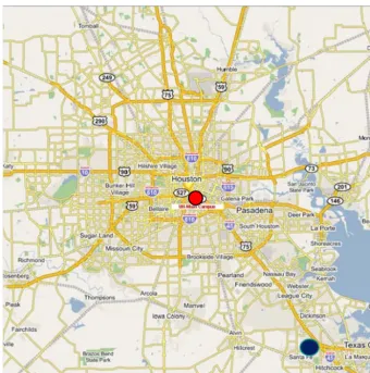
Figure 1. Location of model and measurements. The dark blue dot represents the UH Coastal Center and the red dot represents the UH main campus where the radiosondes were launched.

modeling and observation data were extracted from this lo-cation with the exception of the radiosondes, which were launched from the UH main campus (Rappenglück et al., 2008), and wind fields for the inner WRF domain, which were provided by the Texas Commission on Environmental Quality (TCEQ) Continuous Ambient Monitoring Stations (CAMS) in the surrounding area.

2.2 Observational data

2.2.1 Measurement tower instrumentation

During the study period 28–31 August 2006, both stan-dard and energy budget surface variables were being mea-sured (Table 1). Instrumentation included an R. M. Young 5103 anemometer to capture 10 m wind speeds (WDIR10) and directions (WSPD10), a Campbell Scientific, Inc. (CSI) CS-500 probe for 2 m temperature (TEMP2) and 2 m wa-ter vapor mixing ratio (Q2), and a Kipp & Zonen CNR1 four-component net radiometer to capture incoming short-wave (SWDOWN), incoming longshort-wave (LWDOWN), out-going shortwave (SWUP), and outout-going longwave radiation.

Table 1. Variable names and descriptions for the study.

Variable name (units) Description

TEMP2 (◦C) Temperature at 2 m

Q2 (g kg−1) Water vapor mixing ratio at 2 m WSPD10 (m s−1) Wind speed at 10 m

WDIR10 (◦) Wind direction at 10 m LHFLUX (Wm−2) Latent heat flux at surface SHFLUX (Wm−2) Sensible heat flux at surface GRNDFLUX (Wm−2) Ground flux at surface

SWDOWN (Wm−2) Shortwave incoming radiation at surface LWDOWN (Wm−2) Longwave incoming radiation at surface SWUP (Wm−2) Shortwave outgoing radiation at surface USTAR (m s−1) Friction velocity

PBLH (m) Planetary boundary layer height

(4)

2696 C.-S. M. Wilmot et al.: MM5 v3.6.1 and WRF v3.2.1 model comparison measured using Radiation and Energy Balance System

(REBS) soil heat flux plates.

Measurements were taken at a frequency of 1 Hz and averaged to 1 min (TEMP2, Q2, WSPD10, WDIR10) and 10 min (SWDOWN, LWDOWN, SWUP, SHFLUX, LH-FLUX, GRNDFLUX). All measurements were then aver-aged to 1 h to compare to the hourly model data.

2.2.2 Radiosonde data

Radiosondes were not directly measured at the UH-CC dur-ing this study period, but were regularly launched from the UH main campus approximately 40 km away. RS-92 GPS sondes were used (Rappenglück et al., 2008). The difference in potential temperature vertical lines between the grid point representing the UH-CC and the UH was zero, which gave confidence that PBL heights measured at UH provide a rea-sonable approximation for model comparison at the UH-CC. Launches were performed at 06:00 CST and 18:00 CST for the first 2 days of the study period, and more were launched during the final 2 days of the study (Table 2). PBL heights were determined to be the height at which potential temper-ature begins to increase (Rappenglück et al., 2008). The first radiosonde launch was discarded for purposes of statistical analysis because it corresponded to the model initialization time step, which had a value of 0.

2.3 WRF model

The WRF model used for the simulation was the Advanced Research WRF (WRF-ARW) model version 3.5.1 with the following physics configuration: WSM-3 class simple ice microphysics scheme (Hong et al., 2004), Dudhia shortwave radiation scheme (Dudhia, 1989), rapid radiative transfer model (RRTM) longwave radiation scheme (Mlawer et al., 1997), Yonsei University (YSU) (Hong et al., 2006) PBL scheme, and the MM5 land surface scheme (Noah LSM). The specific parameters of Noah LSM for the UC-CC site are listed in Table 3. The land surface data from the United States Geological Survey (USGS) were used. In past air qual-ity studies in Houston we used YSU and found promising results (Czader et al., 2013), and recent intercomparisons with other PBL schemes for the same area showed that YSU simulates vertical meteorological profiles as satisfactorily as the Asymmetric Convective Model version 2 (ACM2); the Mellor–Yamada–Janjic (MYJ) and quasi-normal scale elimi-nation (QNSE), but may be the best to replicate vertical mix-ing of ozone precursors (Cuchiara et al., 2014). The cumulus scheme is set to be identical to the MM5 one, which is de-scribed below.

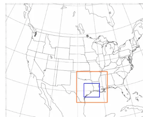
The model was run on three nested domains using one-way nesting (Fig. 2). The horizontal grid scales were the 36 km CONUS domain, 12 km eastern Texas domain, and the 4 km Houston–Galveston–Brazoria domain. All simula-tion results are taken from the 4 km domain grid cell centered

Figure 2. Nesting domain for WRF and MM5 model. The blue box is the 4 km domain that all model outputs were extracted from.

over the UH Coastal Center (Fig. 1) and is thus a point-to-grid cell comparison. The 90 % boundaries of the footprint of the observations fall within this grid cell. No observational nudging was used to avoid any potential effects introduced by nudging procedures. The model was initialized at 00:00 UTC on 28 August 2006 and ended at 23:00 UTC on 1 Septem-ber 2006. The North America Mesoscale (NAM) model was used as meteorological input.

2.4 MM5 model

In order to examine any improvements made from the MM5 to WRF simulations, data extracted from an MM5 simulation were used for a baseline comparison for the Houston case (Table 4). Similarly to previous studies by Ngan et al. (2012) for TexAQS-II in Houston, we applied MM5, version 3.6.1. The physics options included the Medium-Range Forecast (MRF; Hong and Pan, 1996) PBL scheme, Noah LSM, sim-ple ice microphysics scheme, and RRTM radiation scheme. The USGS land use data were used. No observational nudg-ing was used. The same horizontal grid scale as for WRF was used. The cumulus parameterization is set to Grell–Devenyi ensemble scheme (Grell and Devenyi 2002) for 36 km do-main, Kain–Fritsch scheme (Kain, 2004) for 12 km and none for 4 km domain. The choice of no cumulus in 4 km is to suppress the unwanted fake thunderstorms frequently pop-ping up in the model. For MM5 the Eta Data Assimilation System (EDAS) was used.

2.5 Differences between the WRF and MM5 configurations

(5)

Table 2. Radiosonde launch times (CST).

27 Aug 2006 28 Aug 2006 29 Aug 2006 30 Aug 2006 31 Aug 2006 1 Sep 2006

18:00 06:00 06:00 06:00 04:00 04:00

18:00 18:00 12:00 06:00 06:00

18:00 09:00 09:00

12:00 12:00

15:00 15:00

18:00 21:00

Total no. of radiosondes: 20

Table 3. Noah LSM parameters used for the UH-CC site in the MM5 and WRF simulations.

Parameter Meaning Value Category

LU_INDEX IVGTYP Land use index vegetation type 2 Dryland cropland and pasture

ISLTYPE Soil type 12 Clay

VEGFRAC Vegetation fraction 55.20

SHDFAC Green vegetation fraction 0.80

LAI Leaf area index 4.96

EMISS Emissivity 0.97

ALBEDO Albedo 0.18

Z0 Roughness length 0.07

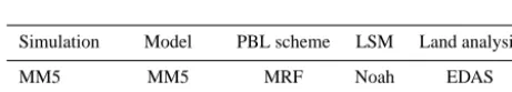
Table 4. Model simulation configurations.

Simulation Model PBL scheme LSM Land analysis

MM5 MM5 MRF Noah EDAS WRF WRF-ARW YSU Noah NAM

related subsequent processes. Cloudiness represented by cor-responding schemes in WRF and MM5 is likely associated with some higher degree of uncertainty. For instance, cloud fraction in a grid box is assumed either 0 or 1 (Dudhia, 1989), which is certainly not precise enough. Unfortunately, in our study we did not have quantitative information about observed cloudiness, and thus we were not able to perform validation studies for these schemes. The EDAS and NAM land surface data sets are similar and use similar observa-tional techniques for data interpolation, but the EDAS runs every 3 h, which allows for higher-resolution temporal in-terpolation than the NAM data, which only runs every 6 h (EDAS Archive Information, National Weather Service En-vironmental Center). Using a more high-resolution data set should lead to better first-guess and ongoing simulations in MM5.

The YSU and MRF PBL schemes use nonlocal closure and rely heavily on the Richardson number (Ri) to compute PBL height for different regimes (e.g., stable, unstable, and neutral PBLs). Both of these PBL schemes essentially define PBL height as the height at which a critical Ri is reached: 0.5 for

the MRF scheme and 0.0 for the YSU scheme (Skamarock et al. 2008). For unstable conditions the PBL height in the YSU scheme is determined to be the first neutral level based on the bulk Richardson number calculated between the lowest model level and the levels above (Hong et al. 2006). 2.6 Statistical analysis

2.6.1 Calculated statistics

For the purposes of this study, the coefficient of determina-tion (r2), the root mean square error (RMSE) and bias are displayed. The RMSE describes the magnitude of the dif-ference between predicted and observed values. Ther2 in-dicates the proportionate amount of variation in the response variableyexplained by the independent variablesxin the lin-ear regression model. The larger ther2, the more variability is explained by the linear regression model. Ther2was cal-culated using a linear model in Matlab. The bias and RMSE was determined as follows:

BIAS=1 n

X

(Y0−Y ), (1)

RMSE=

r

1 n−1

X

(Y0₋_{Y )}2_, ₍₂₎

(6)

2698 C.-S. M. Wilmot et al.: MM5 v3.6.1 and WRF v3.2.1 model comparison

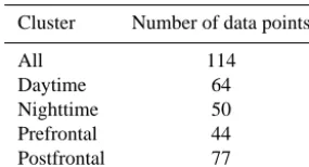
Table 5. Data clusters.

Cluster Number of data points

All 114

Daytime 64

Nighttime 50

Prefrontal 44

Postfrontal 77

2.6.2 Determination of additional statistic groups Hourly values were collected from 00:00 CST on 28 August to 17:00 CST on 1 September, resulting in 114 data points (Table 5). Biases andr2values were evaluated for the com-plete data set as well as for diurnal and frontal clusters. For the diurnal statistics, daytime referred to any data between 06:00 CST and 18:00 CST. Rappenglück et al. (2008) dis-cussed the frontal passage that occurred during this period, which occurred during the evening of 29 August. An exam-ination of the meteorology shows that generally southerly winds gave way to sustained northerly winds on 29 Au-gust around 18:30 CST, indicating this frontal passage. For the purposes of this study, the prefrontal period runs from 00:00 CST on 28 August to 19:00 CST on 29 August, and the postfrontal period runs from 20:00 CST on 29 August to 17:00 CST on 1 September.

3 Results and discussion

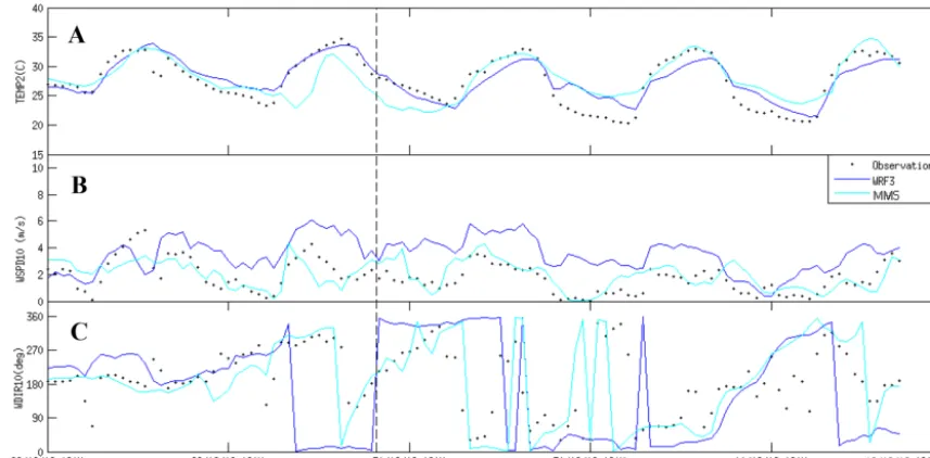
3.1 Standard meteorological variables 3.1.1 Temperature

WRF has the highest r2 for all of the study period as well as when the data are separated into daytime, nighttime, pre-frontal, and postfrontal time periods (Table 6). The largest differences between the WRF and MM5 model in the r2 value occur at night and during prefrontal conditions, both of which have differences of 0.53. However, the nighttimer2 value for MM5 was the smallest at 0.04, which reflects the variability in the nighttime temperature modeling. The WRF model has a higher nighttimer2value of 0.57, but this value also represents the smallestr2value for the model, which im-plies that both models have difficulty getting nighttime tem-peratures correct. Batching the data into prefrontal and post-frontal groups had little effect on ther2values for WRF, but led to increased values in both of the MM5 models.

WRF and MM5 have about the same magnitude bias for the entire study period, but WRF has larger biases for the daytime and nighttime, while WRF has lower biases for pre-frontal period, and in particular for the postpre-frontal period. The overall biases for all of the simulations are relatively low, but both WRF and MM5 underestimate temperatures

by about half a degree during the day and overestimate tem-peratures by about one and a half degree at night for the entire study period (Table 6). These biases could possibly be attributed to too much moisture in the models, which would suppress temperature amplitudes. This warm night-time bias is especially evident on the nights of 30 and 31 Au-gust (Fig. 3). These biases could be the product of too much moisture in the model, which would lead to less suppressed temperature peaks. Another possibility is that there is too much nighttime surface energy in the model, which could lead to increased nighttime temperatures. Also, higher mod-eled nighttime winds could lead to a well-mixed nighttime atmosphere, which would prevent temperatures from drop-ping as low as they should in the model.

Steeneveld et al. (2010) noted that both of the models have difficulty simulating nighttime temperatures. That same study also mentioned that the MM5 warming and cooling trends tended to lag behind the observations, which is visi-ble in the time series for the first half of this study as well (Fig. 3). The WRF model simulation does not have this same time lag.

3.1.2 Water vapor

WRF r2 values for water vapor are lower than the MM5 r2values (Table 6). The overall r2values were highest for MM5, while the daytime r2 values were highest for both WRF and MM5. MM5 had the highest overall and post-frontal values. Both of the models saw lowr2 values prior to the frontal passage, which only increased for MM5 fol-lowing the frontal passage. WRF had the lowest postfrontal and prefrontal values. The water vapor mixing ratior2values are relatively high for MM5 although they are lower than the temperaturer2values. For WRF these values are consistently lower than the temperaturer2 values. Daytime water vapor mixing ratio tended to be higher than the overallr2, while nighttime water vaporr2values were slightly lower than the overallr2for MM5, but significantly lower for WRF. MM5 overall, daytime, and nighttimer2 values were higher than WRF. This is even more evident for the prefrontal and post-frontal conditions.

(7)

Table 6. Results forr2 and bias for all, diurnal, and frontal conditions for temperature (TEMP2), water vapor mixing ratio (Q2), wind speed (WSPD10), wind direction (WDIR), incoming longwave radiation (LWDOWN), outgoing shortwave radiation (SWUP), and incoming shortwave radiation (SWDOWN).

TEMP2 Q2 WSPD10 WDIR10 LWDOWN SWUP SWDOWN

WRF MM5 WRF MM5 WRF MM5 WRF MM5 WRF MM5 WRF MM5 WRF MM5

r2 0.78 0.56 0.37 0.73 0.28 0.40 0.02 0.29 0.52 0.64 – – – –

r2_Day 0.71 0.48 0.64 0.78 0.17 0.31 0.00 0.50 0.66 0.61 0.71 0.23 0.75 0.64

r2_Night 0.57 0.04 0.10 0.66 0.09 0.45 0.09 0.03 0.31 0.47 – – – –

r2_Prefront 0.79 0.36 0.00 0.31 0.16 0.33 0.04 0.30 0.59 0.45 0.86 0.65 0.86 0.64 r2_Postfront 0.79 0.65 0.00 0.56 0.44 0.45 0.06 0.27 0.15 0.48 0.88 0.76 0.91 0.92

Bias 0.24 0.23 −1.44 −2.61 1.70 0.18 −21.48 −2.41 0.34 3.00 – – – –

Bias_Day −0.71 −0.62 −1.47 −2.81 1.69 −0.11 −37.89 −8.32 −5.46 2.76 15.93 60.49 77.85 17.04

Bias_Night 1.46 1.33 −1.40 −2.36 1.72 0.54 −0.47 5.17 7.78 3.30 – – – –

Bias_Prefront 0.59 −0.73 −1.32 −2.77 1.35 −0.08 −35.82 −10.23 6.16 4.35 11.27 79.12 61.38 −24.00 Bias_Postfront 0.02 0.84 −1.51 −2.51 1.93 0.34 −12.47 2.51 −3.31 2.15 6.29 4.38 32.58 30.65

RMSE 1.95 2.71 2.76 3.00 2.08 0.97 145.97 94.58 15.36 14.41 – – – –

RMSE_Day 1.76 2.41 2.35 3.17 2.09 0.99 164.63 83.61 14.40 15.37 36.44 122.92 180.32 205.03

RMSE_Night 2.18 3.06 3.21 2.78 2.07 0.94 117.85 107.00 16.52 13.08 – – – –

RMSE_Prefront 1.58 2.75 2.28 3.10 1.97 1.08 130.75 59.73 14.26 15.86 29.38 141.81 154.04 199.07 RMSE_Postfront 2.16 2.69 3.03 2.94 2.15 0.89 154.77 111.02 16.02 13.41 25.96 34.28 121.71 116.30

to be affected by more than the water vapor mixing ratios. For the 2 days following the frontal passage, the models’ temperature and water vapor mixing ratio biases appear to be more coupled. WRF underestimates daytime temperature with a bias of−3.31◦C and could correspond to a moist bias of−3.05 g kg−1, while MM5 slightly overestimates daytime temperature with a bias of 0.12◦C and could correspond to a moist bias of−2.65 g kg−1. The days following the frontal passage were mostly cloudless, so temperature may be more directly affected by moisture. The fact that following the frontal passage the conditions are more dry could also be a contributing factor, as the observed water vapor mixing ratio dropped by approximately 4 g kg−1_{for the remainder of the} study period (figure not shown). Moisture bias effects could be magnified in light of much smaller moisture values.

For the 2 nights following the frontal passage, both mod-els’ dry biases are relatively close to the mean nighttime bi-ases of the entire study period, but temperature bibi-ases are not proportional to these changes. The nighttime biases decrease by 0.84 g kg−1and 0.09 g kg−1for WRF and MM5, respec-tively, but both models clearly overestimate temperature on the nights of 30 and 31 August (Fig. 3). For the entire study period, the models have too warm nighttime biases of 1.46◦C and 1.33◦C for WRF and MM5, respectively; these warm bi-ases increase to 2.22◦C and 2.61◦C for those 2 nights. 3.1.3 Wind speed

Wind speeds had generally low r2 values, with the highest overallr2being the MM5 simulation using EDAS (Fig. 3). Separating data into day- and nighttime values did not in-crease ther2values; in fact, both day- and nighttimer2were lower than the overall values for both of the models. While the MM5 model bias was relatively small and slightly un-derestimated during the daytime, the WRF model

overesti-mated with a much higher magnitude. Both models have the largest biases at night when wind speeds are overestimated, and with the highest overestimation occurring by the WRF model. Ngan et al. (2012) mention that modeled MM5 winds persisted for hours after the observed winds had died down at sunset. A similar trend is visible for a few nights of this study period in MM5, but is most clearly evident in the WRF model.

(8)

Figure 3. Time series of temperature (a), wind speed ((b), and wind direction (c) for observations (dots) and for the WRF (blue) and MM5 with EDAS (green) models. The dotted line marks the beginning of postfrontal conditions.

3.1.4 Wind direction

Wind direction r2 values were generally low for the entire study period and at nighttime for both models, and only reach approximately 0.50 during the daytime (Table 6). Houston’s proximity to the Gulf of Mexico generally means that there is a strong diurnal cycle as the temperature difference be-tween the land and the water creates surface pressure gradi-ents. This cycle tends to manifest itself in strong southerly winds during the daytime and more northerly winds in the evening and at night. However, during this time period the frontal passage led to more persistent northerly winds, which might have interfered with the normal cycle of the models (Fig. 3). The prefrontal and postfrontal r2 values are both with values at or near 0.30 for MM5 and below 0.10 for WRF. During the study period, wind direction was variable as the front and the daytime wind cycle came into contact.

The magnitudes for the overall, daytime, and nighttime bi-ases were an order of magnitude larger for WRF than for MM5 in most cases. Wind direction for the entire study was underestimated by 21.48◦and 2.41◦in WRF and MM5, re-spectively, which means that the wind directions were in the same quadrant, but for WRF started having more of an or-thogonal wind component. During the daytime these bias magnitudes increase for both models. This could possibly be related to the frontal passage, especially during the day when the frontal passage and the land–sea breeze cycle led to stagnant air conditions and wind directions were variable. Southerly winds are associated with moist, ocean air, while north and northwesterly winds are associated with drier, con-tinental air, so the direction of the wind in the models could

relate to the level of water vapor mixing ratio found in the models.

3.2 Energy budget variables 3.2.1 Radiation

Longwave outgoing radiation is only available at the top of the atmosphere, not at the surface, for both WRF and MM5. As we restricted our analysis to the available model outputs at the surface only, this variable was removed from the study analysis, and only the other three components of radiation were studied (Table 6).

Incoming longwave radiation

Ther2values for longwave radiation are often lower than for either temperature or water vapor mixing ratio, but are still relatively high (Table 6). WRF has a higherr2 during the daytime than overall, while MM5 is slightly lower than the overall value during the daytime. The overall and daytime WRFr2values are about the same as the MM5 values, but at night MM5 has a slightly higherr2than the WRF model. Both models have relatively low nighttimer2 values com-pared to either daytime or overall values.

(9)

Figure 4. Time series for incoming longwave (a), outgoing shortwave (b), and incoming shortwave (c) radiation for observations (dots) and for the WRF (blue) and MM5 with EDAS (green) models.

There is a slight time lag in both the cooling and the warm-ing trends for the longwave radiation for both models, but they both also attempt to capture the drop in radiation fol-lowing the frontal passage (Fig. 4). Both of the models over-estimated; prefrontal conditions produced the largest bias. In MM5 there is an almost 50 % drop in bias from the prefrontal to postfrontal data cluster, and a WRF even changed to under-estimation. WRF had the lowest overall, but highest frontal cluster biases.

Incoming/outgoing shortwave radiation

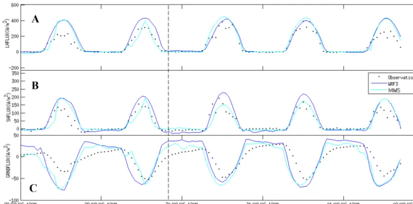
The models treat outgoing radiation as a direct decrease caused by albedo. Therefore, both incoming and outgoing shortwave radiation are driven to 0 after sunset, leading to the “−” found in the tables for nighttime values. For outgo-ing radiation, the WRF model performs better than the MM5 model, which has very small r2 values during the daytime (Table 6). These smallr2values are most likely the result of the overestimations found during the early part of the study period when MM5 overestimates outgoing shortwave radia-tion by as much 337 Wm−2(Fig. 4) and results in daytime biases of 60 Wm−2_{. This is a puzzling feature as it is not} a consistent behavior. It predominantly occurs on the 2 pre-frontal days. Also, the occurrence of these large deviations of SWUP in MM5 is accompanied by concurrent underpre-diction of SWDOWN in MM5; often these underpreunderpre-dictions in SWDOWN are of the similar magnitude as the overpre-dictions in SWUP, which points to a deficient energy distri-bution in MM5 on these days. Regardless of the nature of this deficiency, its impact is visible in corresponding under-predictions in the fluxes of sensible and latent heat (Fig. 5),

and to some extent it is also reflected in the temperature time series (Fig. 3). The significant PBL underprediction in MM5 on 29 August (see discussion on PBL in Sect. 3.3) is likely due to the underprediction of sensible and latent heat in MM5 on that day (Fig. 5), which in turn might be associated with the deficient simulation of incoming and outgoing shortwave radiation by MM5 on the same day. While the overall flux in the WRF model is slightly overestimated, it is overestimated in MM5 with a magnitude of 33 Wm−2_.

For the first 2 days of the study period, incoming solar radiation (SWDOWN) did not reach maximum insolation peaks, possibly due to scattered cloud cover. Following the frontal passage on 29 August, cloud cover began to dissi-pate as observed incoming solar radiation began to increase, reaching maximum insolation on the afternoon of 31 Au-gust before again devolving on 1 September. However, both models moved too soon in developing maximum insolation (Fig. 4).

During the daytime for the entire study period, both mod-els tended to overestimate SWDOWN (Table 6). However, for the 2 clearest days of the study period, both WRF and MM5 overestimated incoming solar radiation by 75.5 Wm−2 and 52.9 Wm−2_{, respectively. While these values drop to} 16.25 Wm−2 _{and 17.27 Wm}−2 _{on the clearest day of the} study, both models continue to overestimate incoming solar radiation. This excess energy in the models could appear as overestimations in the energy flux partitions for sensible, la-tent, and ground flux.

(10)

Figure 5. Time series for latent heat (a), sensible (b), and ground (c) flux for observations (dots) and for the WRF (blue) and MM5 with EDAS (green) models.

biases for incoming radiation are smaller for MM5, while the magnitudes of the biases for outgoing radiation are smaller for WRF (Table 6).

For both outgoing and incoming radiation, daytimer2 val-ues and biases could be affected by the delayed onset of day-time radiation in the models. Both models take an additional hour before seeing increased incoming and outgoing solar radiation values, which is especially visible following the frontal passage (Fig. 4). The averaging of the hourly obser-vations when sunrise occurred in the middle of an hour may also contribute to the discrepancy between the observations and simulations. Incoming solar radiation has much smaller biases. The maximum daytime values reached 979 Wm−2, leading to a maximum daytime average bias of only 1%.

Similar to the outgoing shortwave radiation, both model runs for incoming shortwave radiation have larger postfrontal r2 values (Table 6). Both of the models have comparable postfrontalr2values, but WRF has higher prefrontalr2 val-ues. While WRF overestimated, MM5 underestimated prior to the front, but both models overestimated similarly follow-ing the front. WRF had the largest bias in the prefrontal clus-ter.

3.2.2 Flux variables Latent heat flux

The overall latent heat fluxr2values for both simulations are even higher than for temperature, but decrease when consid-ering the daytime values and become almost negligible when considering the nighttime values (Fig. 5). WRF again has the highest r2values for most of the groupings. When looking

at the frontal passage period, the data tend to have a highr2 during the postfrontal period (Table 7).

In most cases the WRF model has a larger bias magnitude than the MM5 model (Table 7). Overall and daytime latent heat flux is overestimated for both of the models with the largest biases occurring during the daytime. The nighttime biases for both of the models are relatively small. They are underestimated in MM5, but overestimated in WRF.

Prior to the frontal passage on 29 August, latent heat val-ues were scattered throughout the day, which could cor-respond to lower moisture content (Fig. 5). Following the frontal passage (30 and 31 August), observed daytime latent heat flux increases, indicating increased moisture. Both mod-els overestimate daytime latent heat flux for the entire study period, but WRF has larger overestimations than MM5 by approximately 20 Wm−2(Table 7). However, on 30 and 31 August both models perform similarly with overestimation biases of∼21 Wm−2and∼17 Wm−2for WRF and MM5, representing a difference of 6 Wm−2. Both models vary in their simulation of the meteorological conditions prior to the frontal passage but resort to similar parameterizations fol-lowing the front, perhaps in response to the clearer incoming solar radiation simulations.

Sensible heat flux

(11)

Table 7. Results forr2and bias for all, diurnal, and frontal conditions for latent heat flux (LHFLUX), sensible heat flux (SHFLUX), ground flux (GRNDFLUX), and friction velocity (USTAR).

LHFLUX SHFLUX GRNDFLUX USTAR

WRF MM5 WRF MM5 WRF MM5 WRF MM5

r2 0.88 0.87 0.89 0.77 0.68 0.67 0.73 0.70

r2_Day 0.75 0.75 0.81 0.64 0.51 0.47 0.62 0.56

r2_Night 0.37 0.00 0.08 0.16 0.03 0.13 0.26 0.11

r2_Prefront 0.92 0.75 0.89 0.71 0.58 0.60 0.61 0.61

r2_Postfront 0.89 0.92 0.90 0.81 0.74 0.70 0.81 0.77 Bias 42.31 26.99 14.32 3.75 −5.82 −10.52 0.15 0.02 Bias_Day 73.29 49.84 32.92 6.83 −46.70 −47.40 0.18 0.01 Bias_Night 2.65 −2.27 −9.48 −0.21 46.50 36.68 0.11 0.03 Bias_Prefront 60.96 16.46 21.00 5.39 −14.50 −15.72 0.15 0.00 Bias_Postfront 30.58 33.61 10.12 2.71 −0.37 −7.25 0.14 0.02

RMSE 77.77 70.62 38.89 31.5 60.85 56.09 0.17 0.08

RMSE_Day 103.7 94.04 50.76 41.52 69.33 66.35 0.20 0.08 RMSE_Night 5.18 7.11 12.29 7.48 47.86 39.23 0.14 0.06 RMSE_Prefront 94.26 74.02 40.94 35.30 56.22 49.93 0.19 0.09 RMSE_Postfront 65.32 68.40 37.55 28.86 63.59 59.64 0.16 0.07

For the study period there was an r2 value of 0.49 be-tween observed sensible heat flux and water vapor mixing ratio at night. None of the models reach this level ofr2 val-ues, but the MM5 models get closer to this relationship than the WRF model. The decrease inr2from sensible heat flux to latent heat flux and the decrease in the magnitude of the bi-ases in MM5 are in agreement with the findings of Zhong et al. (2007). The WRF results agree with LeMone et al. (2009), who found that their modeled sensible heat overestimated throughout the entire study period; however, our results show lower bias for sensible heat than latent heat, which is in disagreement with the LeMone study. WRF had the higher overall, nighttime, and daytime biases than MM5. WRF and MM5 overestimated sensible heat flux for all clusters with the exception of nighttime. While ther2decreased for sen-sible heat flux compared to latent heat flux and the biases are smaller, the relative magnitude of the biases represents a larger portion of measured values. During the daytime, MM5 had an average overestimation of 7 % while WRF overesti-mated by 33 %. This is a 26 % disparity between the values during the daytime, but this gap decreases greatly at night, when WRF underestimated values by as much as 9 % while MM5 showed almost no bias. However, WRF shows much better daytime values for r2 and RMSE than MM5, which compensates for the poor WRF bias values to some extent.

The sensible heat flux shows a similar simulation pattern to the latent heat flux time series (Fig. 5). During the first 2 days of the study period, both models respond differently to the in-consistent sensible heat flux, but have similar responses dur-ing the 2 days followdur-ing the frontal passage. Overall, Fig. 5 reflects the higher daytime biases for WRF compared with MM5 (Table 7). Sensible heating is associated with ground heating, so it is possible that temperature variations in the

models, combined with differences in the moisture, could contribute to these variations. However, the 2 days following the frontal passage produce similar model responses, with WRF and MM5 overestimating sensible heat by∼6 Wm−2,. Ground flux

Similar to the other flux variables, the overallr2values were higher than either the daytime or nighttime values (Table 7). Out of all the flux variables, the overall and daytimer2values for ground flux are the lowest. The nighttimer2values are also very low. The WRF model has slightly higherr2values than the MM5 model overall and during the day, but is lower at night.

(12)

Figure 6. Time series for friction velocity.

3.2.3 Turbulence

Friction velocity, or u∗, is one measure of how much tur-bulence is being generated through shearing forces at any given time (Stull, 1988). Examining the observed and mod-eled and measured values can provide insight into shear tur-bulence that contributes to the development of the PBL. Ta-ble 7 presents the overall and diurnalr2and bias values for friction velocity, and Fig. 6 shows the time series for the study period.

Despite the fact that friction velocity is a small compo-nent of turbulent energy, the models are able to model it rel-atively well with overallr2values of 0.73 and 0.70 for WRF and MM5, respectively. The overallr2values for both of the models are higher than daytime values and much higher than the nighttime values. At night, the models are set to a min-imum value of 0.1 m s−1_{, which does not always accurately} reflect the observations that can get much smaller. Above this threshold, both models attempt to mimic nighttimeu∗ behav-ior, but following the frontal passage, nighttime wind speeds were relatively calm (Fig. 3). On those nights observed u∗ values were well below the 0.1 m s−1 threshold, so neither model is able to simulate these values, which could have led to the low nighttimer2values.

Both models overestimate u∗, which could be related to the overestimations in wind speed for the models. There is no distinct cluster with the highest bias magnitudes; the largest bias for WRF occurs during the daytime but for MM5 occurs at night. WRF has the highest overall, daytime, and night-time magnitude biases, which is in contrast with Hanna et al. (2010), who mentioned that MM5 had larger biases in the afternoon than WRF. Friction velocity is a measure of how much shear turbulence will be generated and is affected by topography and is directly related to wind speed. Compared to the other model variables, the absolute biases for friction velocity are relatively small, but assuming a maximum u∗ value of approximately 0.6 m s−1, the bias can be overesti-mated by nearly 30 % in the WRF model.

3.3 Planetary boundary layer

Due to the small number of radiosonde launches available for the duration of the study period, the biases were not calculated for planetary boundary layer height. However,

PBL heights were calculated at sunrise and sunset prior to the frontal passage, and then following the frontal passage were recorded with more regularity, so the few observa-tions available offer a better chance to look at the develop-ment and destruction of the PBL (Fig. 7). Ideally, suppressed daytime temperatures and elevated nighttime temperatures should yield similar PBL height results. However, while the daytime PBL heights are in fact underestimated during the day as expected, they are also often underestimated at night when they should be overestimated. Daytime peaks are bet-ter approximated following the frontal passage, but the PBL destruction always happens too soon.

There are various reasons for the possible variations in the onset of PBL development and destruction. Especially dur-ing the morndur-ing PBL height estimates, the late onset of solar radiation in the models could contribute to the slow devel-opment of the PBL during a time when convection leads to a rapid increase of PBL height. LeMone et al. (2009) sug-gest overestimations of sensible heat lead to overestimations in the convective boundary layer depth. In general, MM5 has the smallest underestimations and overestimations. How-ever, both models replicate PBL height estimations reason-ably well, with a few exceptions though: on 29 August, both models do not capture the maximum PBL height, with MM5 significantly failing, while on 1 September, MM5 performs quite well and WRF only reaches about 50 % of the observed PBL height. The significant PBL underprediction in MM5 is likely due to the underprediction of sensible and latent heat in MM5 on that day (Fig. 5), which in turn might be associ-ated with the deficient simulation of shortwave radiation by MM5 on the same day.

(13)

Figure 7. Comparison of observed and simulated PBL height for the study period. The WRF simulation tended to underestimate more than either of the MM5 simulations.

ozone concentrations, so it is no surprise that using MM5 simulations as a meteorological driver for air quality mod-eling led to underestimation of ozone on 31 August and 1 September by 25–30 ppb (Banta et al., 2011; Ngan et al, 2012).

4 Conclusions

Although WRF v3.5.1 does not perform as well as MM5 v3.6.1 in predicting PBL heights, it does a better job in cap-turing energy budget and most of the general variables (with exception of wind speed/direction and water vapor mixing ratio). Energy balance partitioning can have an effect on stan-dard and planetary boundary layer height variables. Both models overestimate incoming solar radiation, which implies a surplus of energy that could be exhibited in either the par-titioning of the surface energy variables or in some other as-pect of the meteorological modeling not examined here. This scenario would also imply that there is more energy avail-able for the nighttime system, which should mean increased temperatures and higher boundary layer height estimations. While nighttime temperatures seem to reflect this increased energy for both models, PBL height estimations only reflect it in WRF.

The nighttime temperature bias disparity in the models fol-lowing the frontal passage could reflect the disparity in mois-ture. The MM5 model consistently had much drier condi-tions than the WRF model, which could mean more energy available to other parts of the meteorological system. On the clearest day of the study period MM5 had increased latent heat flux, which could lead to higher evaporation rates and lower moisture in the model. However, this latent heat dis-parity between the two models is not visible during any other part of the study, so examining sequential cloud-free days would be necessary to see whether the moisture and latent heat effect was sustained. The full effects of moisture on the energy balance cannot be determined here other than as a

po-tential reason for inconsistent model outputs. The differences in the land data sets used to initialize and update each model make this situation plausible.

The frontal passage allowed this study to examine these variables both under prefrontal and postfrontal conditions, and it was found that a frontal passage affects the perfor-mance of most of the variables, including the radiation, flux, and turbulence variables, at times creating significant differ-ences in ther2 values. Ultimately the clear, sunny days of-fered the most insight into the potential effects of the energy balance variables on standard variables and planetary bound-ary layer height. These 2 days were also 2 of the highest 8 h ozone peak days on record for the year. Since these kinds of days are favorable for high ozone production, the energy balance variables reproduced on these days could more ac-curately represent meteorological conditions. Acac-curately de-termining the energy balance variables could in turn produce better standard meteorology and PBL heights, which are es-sential in determining accurate ozone concentrations.

The results presented in this paper are restricted to the val-idation of one 4 km domain grid cell with observations in this specific grid cell. We do not claim that these validations are valid throughout the domain and for each grid cell as this would require a corresponding network of micrometeorolog-ical observations. However, we believe that a point-to-grid validation on one 4 km domain grid cell may still be helpful in elucidating different behaviors and/or progresses in differ-ent models to simulate boundary layer properties.

Acknowledgements. We are grateful for financial and

infrastruc-tural support provided by the UH-CC, and we would like to thank Dr. Fong Ngan (NOAA-ARL) for valuable discussions.

(14)

2706 C.-S. M. Wilmot et al.: MM5 v3.6.1 and WRF v3.2.1 model comparison References

Air Resources Laboratory: Eta Data Assimilation System (EDAS) Archive Information, available at: http://ready.arl.noaa.gov/ edas80.php (last access: 2 December 2013), 2013.

Banta, R. M., Senff, C., Nielsen-Gammon, J., Darby, L., Ryer-son, T., Alvarez, R., Spandberg, S., Williams, E., and Trainer, M.: A bad air day in Houston, B. Am. Meteorol. Soc., 86, 657–669, 2005.

Banta, R. M., Senff, C., Alvarez, R., Langford, A., Parrish, D., Trainer, M., Darby, L., Hardesty, R., Lambeth, B., Neuman, J., Angevine, W., Nielsen-Gammon, J., Sandberg, S., and White, A.: Dependence of daily peak O3 concentrations near Houston, Texas on environmental factors: wind speed, temperature, and boundary-layer depth, Atmos. Environ., 45, 162–173, 2011. Borge, R., Alexandrov, V., del Vas, J. J., Lumbreras, J., and

Ro-driguez, E.: A comprehensive sensitivity analysis of the WRF model for air quality applications over the Iberian Peninsula, At-mos. Environ., 42, 8560–8574, 2008.

Byun, D. W. and Schere, K.: Review of the governing equations, computational algorithms, and other componenets of the Models-3 community multiscale air quality (CMAQ) modeling system, Appl. Mech. Rev., 59, 51–77, 2006.

Chen, F. and Dudhia, J.: Coupling an advanced land surface hy-drology model with the Penn State-NCAR MM5 modeling sys-tem. Part 1: Model implementation and sensitivity, Mon. Weather Rev., 129, 569–585, 2001.

Clements, C. B., Zhong, S., Goodrick, S., Li, J., Potter, B. E., Bian, X., Heilman, W. E., Charney, J. J., Perna, R., Jang, M., Lee, D., Patel, M., Street, S., and Aumann, G.: Observing the dynamics of wildland grass fires – FireFlux – a field validation experiment, B. Am. Meteorol. Soc., 88, 1369–1382, 2007. Cuchiara, G. C., Li, X., Carvalho, J., and Rappenglück, B.:

Inter-comparison of planetary boundary layer parameterization and its impacts on surface ozone formation in the WRF/Chem model for a case study in Houston/Texas, Atmos. Environ., 96, 175–185, doi:10.1016/j.atmosenv.2014.07.013, 2014.

Czader, B. H., Li, X., and Rappenglück, B.: CMAQ model-ing and analysis of radicals, radical precursors and chem-ical transformations, J. Geophys. Res., 118, 11376–11387, doi:10.1002/jgrd.50807, 2013.

Day, B. M., Rappenglück, R., Clements, C., Tucker, S., and Brewer, W.: Nocturnal boundary layer characteristics and land breeze development in Houston, Texas during TexAQS II, At-mos. Environ., 44, 4014–4023, 2010.

Dudhia, J.: Numerical study of convection observed during the winter monsoon experiment using a mesoscale two-dimensional model, J. Atmos. Sci., 46, 3077–3107, 1989.

Gilliam, R. and Pleim, J.: Performance assessment of new land sur-face and planetary boundar layer physics in the WRF-ARW, J. Appl. Meteorol. Clim., 49, 760–774, 2010.

Grell, G. A. and Devenyi, D.: A generalized approach to pa-rameterizing convection combining ensemble and data as-similation techniques, Geophys. Res. Lett., 29, 38.1–38.4, doi:10.1029/2002GL015311, 2002.

Grell, G. A., Dudhia, J., and Stauffer, D.: A description of the fifth-generation Penn State/NCAR Mesoscale Model (MM5), NCAR Tech. Note NCAR/TN-3981STR, 122 pp., 1994.

Hanna, S. R., Reen, B., Hendrick, E., Santos, L., Stauffer, D., Deng, A., McQueen, J., Tsudulko, M., Janjic, Z., Jovic, D., and Sykes,

R.: Comparison of observed, MM5, and WRF-NMM model-simulated, and HPAC-assumed boundary layer meteorological variables for 3 days during the IHOP field experiment, Bound.-Lay. Meteorol., 134, 285–306, 2010.

Hong, S. Y. and Pan, H. L.: Nonlocal boundary layer vertical diffu-sion in a medium range-forecast model, Mon. Weather Rev., 124, 2322–2339, 1996.

Hong, S. Y., Dudhia, J., and Chen, S. H.: A revised approach to ice microphysical processes for the bulk parameterization of clouds and precipitation, Mon. Weather Rev., 132, 103–120, 2004. Hu, X. M., Nielsen-Gammon, J., and Zhang, F.: Evaluation of three

planetary boundary layer schemes in the WRF model, J. Appl. Meteorol. Clim., 49, 1831–1844, 2010.

Kain, J. S.: The Kain–Fritsch convective parameterization: An up-date, J. Appl. Meteorol., 43, 170–181, 2004.

Kljun, N., Calanca, P., Rotach, M. W., and Schmid, H. P.: A simple parameterisation for flux footprint pre-dictions, Boundary Layer Meteorol., 112, 503–523, doi:10.1023/B:BOUN.0000030653.71031.96, 2004.

Langford, A. O., Tucker, S., Senff, C., Banta, R., Brewer, W., Al-varez, R., Hardesty, R., Lerner, B., and Williams, E.: Convective venting and surface ozone in Houston during TexAQS2006, J. Geophys. Res., 115, D16305, doi:10.1029/2009JD013301, 2010. LeMone, M., Chen, F., Tewari, M., Dudhia, J., Geerts, B., Miao, Q., Coulter, R., and Grossman, R.: Simulating the IHOP_2002 fair-weather CBL with the WRF-ARW-Noah modeling system. Part 1: Surface fluxes and CBL Structure and evolution along the east-ern track, Mon. Weather Rev., 138, 722–744, 2009.

Mao, Q., Gautney, L. L., Cook, T. M., Jacobs, M. E., Smith, S. N., and Kelsoe, J. J.: Numerical experiments MM5-CMAQ sensitiv-ity to various PBL schemes, Atmos. Environ., 40, 3092–3110, 2006.

Mlawer, E. J., Taubman, S., Brown, P., Iacono, M., and Clough, S.: Radiative transfer for inhomogeneous atmosphere: RRTM, a val-idated correlated-k model for the longwave, J. Geophys. Res., 102, 16663–16682, 1997.

National Weather Service Environmental Modeling Center: NAM: the North American Mesoscale Forecast System, avail-able at: http://www.emc.ncep.noaa.gov/index.php?branch=NAM (last access: 24 November 2013), 2013.

Ngan, F. and Byun, D.: Classification of weather patterns and as-sociated trajectories of high-ozone episodes in the Houston– Galveston–Brazoria area during the 2005/06 TexAQS-II, J. Appl. Meteorol. Clim., 50, 485–499, 2011.

Ngan, F., Byun, D., Kim, H. C., Lee, D. G., Rappenglück, B., and Pour-Biazar, A.: Performance assessment of retrospective mete-orological inputs for use in air quality modeling during TexAQS 2006, Atmos. Environ., 54, 86–96, 2012.

Rappenglück, B., Perna, R., Zhong, S., and Morris, G.: An analysis of the vertical structure of the atmosphere and the upper-level meteorology and their impact on surface ozone levels in Houston, Texas, J. Geophys. Res., 113, D17315, doi:10.1029/2007JD009745, 2008.

(15)

Steenveld, G. J., Wokke, M., Zwaaftink, C., Pijlman, S., Heusinkveld, B., Jacobs, A., and Holtslag, A.: Observations of the radiation divergence in the surface and its implication for its parameterization in numerical weather prediction models, J. Geophys. Res., 115, D06107, doi:10.1029/2009JD013074, 2010. Stull, R. B.: An Introduction to Boundary Layer Meteorology, 13th edn., Atmospheric and Oceanographic Sciences Library, Springer Publishers, 1988.

Tucker, S. C., Banta, R., Langford, A., Senff, C., Brewer, W., Williams, E., Lerner, B., Osthoff, H., and Hardesty, R.: Relation-ships of coastal nocturnal boundary layer winds and turbulence to Houston ozone concentrations during TexAQS 2006, J. Geo-phys. Res., 115, D10304, doi:10.1029/2009JD013169, 2010.

Wilczak, J. M., Djalalova, I., McKeen, S., Bianco, L., Bao, J. W., Grell, G., Peckham, S., Mathur, R., McQueen, J., and Lee, P.: Analysis of regional meteorology and surface ozone during the TexAQS II field program and an evaluation of the NMM-CMAQ and WRF-Chem air quality models, J. Geophys. Res., 114, D00F14, doi:10.1029/2008JD011675, 2009.