www.geosci-model-dev.net/8/3975/2015/ doi:10.5194/gmd-8-3975-2015
© Author(s) 2015. CC Attribution 3.0 License.
NCAR_Topo (v1.0): NCAR global model topography generation
software for unstructured grids
P. H. Lauritzen1, J. T. Bacmeister1, P. F. Callaghan1, and M. A. Taylor2
1National Center for Atmospheric Research, 1850 Table Mesa Drive, Boulder, Colorado, USA 2Sandia National Laboratories, Albuquerque, New Mexico, USA
Correspondence to: P. H. Lauritzen (pel@ucar.edu)
Received: 12 May 2015 – Published in Geosci. Model Dev. Discuss.: 22 June 2015
Revised: 30 September 2015 – Accepted: 1 December 2015 – Published: 14 December 2015
Abstract. It is the purpose of this paper to document the NCAR global model topography generation software for un-structured grids (NCAR_Topo (v1.0)). Given a model grid, the software computes the fraction of the grid box cov-ered by land, the grid-box mean elevation (deviation from a geoid that defines nominal sea level surface), and asso-ciated sub-grid-scale variances commonly used for gravity wave and turbulent mountain stress parameterizations. The software supports regular latitude–longitude grids as well as unstructured grids, e.g., icosahedral, Voronoi, cubed-sphere and variable-resolution grids.
1 Introduction
Accurate representation of the impact of topography on at-mospheric flow is crucial for Earth system modeling. For ex-ample, the hydrological cycle is closely linked to topography and, on the planetary scale, waves associated with the mid-latitude jets are very susceptible to the effective drag caused by mountains (e.g., Lott, 1999). Despite the fact that surface elevation is known globally with a high level of precision, the representation of its impact on atmospheric flow in numerical models remains a challenge.
When performing a spectral analysis of high-resolution el-evation data (e.g., black line in Fig. 1), it is clear that Earth’s topography decreases quite slowly with increasing wave number (see also Balmino, 1993; Uhrner, 2001; Gagnon et al., 2006). Consequently, at any practical model resolution there will always be a non-negligible spectral component of topography present near the grid scale and there will always be a non-negligible spectral component of topography
be-low the grid scale (sub-grid-scale component). The resolved scale component is the mean elevation in each grid box h
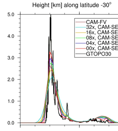
(deviation from a geoid that defines nominal sea level sur-face), or, equivalently (if gravity is assumed constant), the surface geopotential8s. For models using terrain-following coordinates it is common practice not to force the highest wave numbers directly in the model in order to alleviate ob-vious spurious noise (e.g., Navarra et al., 1994; Lander and Hoskins, 1997). Hence, for that class of models,8s is usu-ally smoothed. Figure 1 shows the power spectrum for sur-face elevation for different levels of smoothing of topogra-phy in the NCAR-DOE CESM (Community Earth System Model) CAM (Community Atmosphere Model; Neale et al., 2010) SE (spectral element dynamical core; Thomas and Loft, 2005; Dennis et al., 2005) and CAM-FV (finite-volume dynamical core; Lin, 2004). Figure 2 shows the associated elevations for a cross section through the Andes mountain range. The amount of smoothing necessary is intrinsically linked to the numerical methods and discretization choices in the dynamical core. Further discussion on8s smoothing is given in Sect. 2.2.3.
Figure 1. Log–log plot of spectral energy versus wave number
K for the “raw” 1 km USGS data (GTOPO30), different levels of smoothing for 100 km CAM-SE topography, and CAM-FV. La-bels 04×, 08×, 16×and 32×CAM-SE refer to different levels of smoothing, more precisely 4, 8, 16 and 32 applications of a “Lapla-cian” smoothing operator in SE, respectively. Label CAM-FV refers to the topography used in CAM-CAM-FV at 0.9◦×1.25◦ reso-lution. 00x CAM-SE is the unsmoothed topography on an approx-imately 1◦grid CAM-SE grid. Note that the blue (4×, CAM-SE) and brown (CAM-FV) lines overlap. Solid straight line shows the
K−2slope. The associated surface elevations are shown in Fig. 2.
Webster et al., 2003; Zadra et al., 2003; Kim and Doyle, 2005; Scinocca and McFarlane, 2000) and incorporate the ef-fects of sub-grid-scale topographic anisotropy (i.e., the exis-tence of ridges with dominant orientations used to determine the direction and magnitude of the drag exerted by sub-grid topography). The importance of anisotropy in quantifying to-pographic effects has been recognized for some time (e.g., Baines and Palmer, 1990; Bacmeister, 1993).
According to linear theory, gravity waves can propagate in the vertical only when their intrinsic frequency is lower than the Brunt–Väisälä frequency N (e.g., Durran, 2003). For orographically forced gravity waves the intrinsic fre-quency is set by the obstacle horizontal scale and the wind speed. When obstacle scales are too small to generate prop-agating waves, we expect drag to be produced by unstrati-fied turbulent flow, a process which is typically parameter-ized in models’ TMS schemes. For larger obstacles we ex-pect both drag and vertically propagating waves to result, processes which are dealt with by GWD schemes. Unfor-tunately the scale separating TMS and GWD processes is flow dependent. For typical midlatitude values of low-level
Figure 2. Surface elevation in kilometers for a cross section along latitude 30◦S (through Andes mountain range) for different repre-sentations of surface elevation. The labeling is the same as in Fig. 1.
wind (10 m s−1) andN (10−2s−1), waves with wavelengths less than around 6000 m will not propagate in the vertical. A separation scale of 5000 m has been used by ECMWF (1997) and Beljaars et al. (2004). Here we will generate two sub-grid-scale variables derived from the topography data: the variance of topography below the 6000 m scale (referred to as Var(TMS)) and the variance of topography with a scale longer than 6000 m and less than the grid scale (referred to as Var(GWD)).
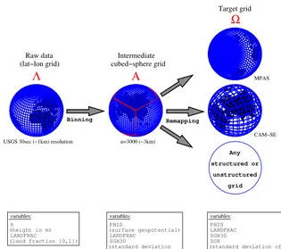
It is the purpose of this paper to document a software pack-age (NCAR_Topo (v1.0)) that, given a “raw” high-resolution global elevation data set, maps elevation data to any unstruc-tured global grid and separates the scales needed for TMS and GWD parameterizations. This separation of scales is done through an intermediate mapping of the raw elevation data to a 3000 m cubed-sphere grid (3→A) before map-ping fields to the target model grid (A→) as schemati-cally shown in Fig. 3. This two-step process is described in Sect. 2.2 after a mathematical definition of the scale separa-tion (Sect. 2.1). In Sect. 2.2.3 we briefly discuss8s smooth-ing (if applicable). Output from the topography software is shown and discussed in Sect. 3.
2 Method
2.1 Continuous: separation of scales
(lat−lon grid)
of 30sec h)
Ω
Target grid
Raw data
Binning
Any
unstructured Remapping
structured or
grid
USGS 30sec (~1km) resolution n=3000 (~3km)
PHIS
variables:
LANDFRAC SGH30 SGH
(standard deviation of ~3km cubed−sphere h) (land fraction [0,1])
LANDFRAC h
(height in m)
variables:
PHIS
(surface geopotential) LANDFRAC
SGH30
variables:
(standard deviation
MPAS
CAM−SE
Α
Λ
cubed−sphere grid Intermediate
Figure 3. A schematic showing the regridding procedure. Red fonts refer to the naming conventions for the grids:3is the “raw” data grid (1 km regular latitude–longitude grid),Ais the intermediate cubed-sphere grid, andis the target grid which may be any unstructured or structured grid. The variable naming convections in the boxes are explained in Sect. 2.3. Data for the variable-resolution MPAS (Model for Prediction Across Scales; Skamarock et al., 2012) grid plot are courtesy of W. C. Skamarock (NCAR).
which case it can be represented by a convergent expansion of spherical harmonic functions of the form
h(λ, θ )=
∞
X
m=−∞
∞
X
n=|m|
ψm,nYm,n(λ, θ ), (1)
(e.g., Durran, 2010) where λ andθ are longitude and lati-tude, respectively, andψm,nare the spherical harmonic
coef-ficients. Each spherical harmonic function is given in terms of the associated Legendre polynomialPm,n(θ ):
Ym,n=Pm,n(θ )eimλ, (2)
wheremis the zonal wave number andm− |n|is the number of zeros between the poles and can therefore be interpreted as meridional wave number.
For the separation of scales the spherical harmonic expan-sion is truncated at wave numberM,
h(M)(λ, θ )=
M
X
m=−M M
X
n=|m|
ψm,n(M)Ym,n(λ, θ ), (3)
where a triangular truncation, which provides a uniform spa-tial resolution over the entire sphere, is used.
Leth(tgt)(λ, θ )be a continuous representation of the eleva-tion containing the spatial scales of the target grid. We do not
writeh(tgt)(λ, θ )explicitly in terms of spherical harmonics as the target grid may be variable resolution and therefore con-tain different spatial scales in different parts of the domain.
For each target grid cellk,k=1, . . ., Nt, whereNtis the number of target grid cells, define the variances
Var(tms)
k =
Z Z
k
h
h(M)(λ, θ )−h(λ, θ )i2cos(θ )dλdθ, (4)
Var(gwd)
k =
Z Z
k
h
h(tgt)(λ, θ )−h(M)(λ, θ )i2cos(θ )dλdθ. (5)
Thus Var(tms)
k is the variance of elevation on scales below
wave numberMand Var(gwd)
k is the variance of elevation on
scales larger than wave numberMand below the target grid scale.
2.2 Discrete: separation of scales
Any quasi-uniform spherical grid could, in theory, be used for the separation of scales or, given the discontinu-ous/fractal nature of topography, a more rigorous scale sep-aration method such as wavelets or other techniques could have been used. It is noted that the separation of scales through an intermediate grid does not correspond exactly to a spectral transform truncation (used in the previous sec-tion). The intent is to approximately eliminate scales below what can be resolved on the intermediate grid. For reasons that will become clear, we have chosen to use a gnomonic cubed-sphere grid (see Fig. 3) resulting from an equiangular gnomonic (central) projection,
x=rtanα and y=rtanβ; α, β∈h−π 4,
π
4 i
, (6)
(Ronchi et al., 1996) where α andβ are central angles in each coordinate direction, r=R/
√
3 and R is the radius of the Earth. A point on the sphere is identified with the three-element vector (x, y, ν), where ν is the panel index. Hence the physical domain S (sphere) is represented by the gnomonic (central) projection of the cubed-sphere faces,
(ν)= [−1,1]2, ν=1,2, . . .,6, and the non-overlapping panel domains (ν) span the entire sphere:S=S6
ν=1(ν). The cube edges, however, are discontinuous. Note that any straight line on the gnomonic projection (x, y, ν) corre-sponds to a great-circle arc on the sphere. In the discretized scheme we let the number of cells along a coordinate axis beNcso that the total number of cells in the global domain is 6×Nc2. The grid lines are separated by the same angle
1α=1β= π
2Nc in each coordinate direction.
For notational simplicity the cubed-sphere cells are iden-tified with one index i, and the relationship between iand (icube, jcube,ν) is given by
i=icube+(jcube−1) Nc+(ν−1) Nc2, (7) where (icube, jcube)∈ [1, . . ., Nc]2 and ν∈ [1,2, . . .,6]. In terms of central angles (α, β) the cubed-sphere grid celli
is defined as
Ai = [(icube−1)1α− π
4,icube1α−
π
4] × [(jcube−1)1β−π
4,jcube1β−
π
4], (8)
and 1Ai denotes the associated spherical area. A formula
for the spherical area 1Ai of a grid cell on the gnomonic
cubed-sphere grid can be found in Appendix C of Lauritzen and Nair (2008) (note that Eq. C3 is missing arccos on the right-hand side). A quasi-uniform approximately 3000 m res-olution is obtained by using Nc=3000, which results in a scale separation of roughly 6000 m (based on a simple “21x
assumption”). For more details on the construction of the gnomonic grid see, for example, Lauritzen et al. (2010).
2.2.1 Step 1: raw elevation data to intermediate cubed-sphere grid (3→A)
The raw elevation data are provided on a geoid such as the World Geodetic System 1984 (WGS84) ellipsoid, whose center is located at the Earth’s center. Latitude and longi-tude locations use the WGS84 geodetic datum. Similarly, el-evation above sea level is defined as the deviation from the WGS84 geoid or WGM96 (Earth Geopotential Model 1996) geoid for newer data sets. Global weather/climate models typically assume that Earth is a sphere, so the elevations at a certain latitude–longitude pair on the geoid are taken to be the same on the sphere. The consequences of this approxi-mation in the context of limited-area models are discussed in Monaghan et al. (2013) and in the context of shallow-water experiments in Bénard (2015). Derivation of the equations of motion in more accurate coordinates is starting to emerge in the literature (e.g., White et al., 2008; Gates, 2004; Staniforth and White, 2015).
The “raw” elevation data are usually from a digital eleva-tion model (DEM) such as the GTOPO30, a 30 arcsec global data set from the United States Geological Survey (USGS; Gesch and Larson, 1998) defined on an approximately 1 km regular latitude–longitude grid. Several newer, more accu-rate, and locally higher resolution elevation data sets are available such as GMTED2010 (Global Multi-Resolution Terrain Elevation Data 2010; Danielson and Gesch, 2011), GLOBE (GLOBE Task Team and others, 1999) and the NASA Shuttle Radar Topographic Mission (SRTM) DEM data (Farr et al., 2007). The SRTM data, however, are only near-global (up to 60◦ north and south). Here we use GTOPO30 and GMTED2010. The GTOPO30 data come in 33 tiles (separate files) in 16 bit binary format. Fortran code is provided to convert the data into one NetCDF file. Even though the elevation is stored as integers, the size of the NetCDF file is 7 GB. The GTOPO file contains heighthand land fraction LANDFRAC (for the mathematical operations below we usef to refer to land fraction). The GMTED2010 data do not contain LANDFRAC, so the land fraction is ob-tained from Moderate Resolution Imaging Spectroradiome-ter (MODIS) 1 km land–waSpectroradiome-ter mask data downloaded from ftp://landsc1.nascom.nasa.gov/pub/outgoing/c6_dem/.
The centers of the regular latitude–longitude grid cells for the “raw” topographic data are denoted(λilon, θjlat),ilon= 1, . . ., nlon, jlat=1, . . ., nlat. For the data sets used here
nlon=43 200 andnlat=21 600. As for the cubed sphere, we use one indexjto reference the grid cells,
j=ilon+(jlat−1)×nlon, j∈ [1, . . ., Nr], (9)
whereNr=nlon×nlat. The spherical area of grid cell3jis
denoted13j and the average elevation in cellj is given by h(3raw)
j .
(λilon, θjlat)is located. Due to the “Cartesian-like” structure of the cubed-sphere grid, the search algorithm is straightfor-ward (following Nair et al., 2005):
– Transform (λilon, θilat)coordinate to Cartesian coordi-nates(x, y, z):
x=cos(λilon)cos(θjlat), (10)
y=sin(λilon)cos(θjlat), (11)
z=sin(θilat). (12)
– Locate which cubed-sphere panel(λilon, θilat)is located on through a “coordinate maximality” algorithm, i.e., let pm=max(|x|,|y|,|z|) , (13) then if
– pm= |x|andx >0, then(λilon, θilat)is onν=1; – pm= |y|andy >0, then(λilon, θilat)is onν=2; – pm= |x|andx <0, then(λilon, θilat)is onν=3; – pm= |y|andy <0, then(λilon, θilat)is onν=4; – pm= |z|andz≤0, then(λilon, θilat)is located on
the bottom panel,ν=5;
– pm= |z|andz >0, then(λilon, θilat)is located on the top panel,ν=6.
– Given the panel number the associated central angles
(α, β)are given by
– ν=1:(α, β)=harctanxz,arctanyzi; – ν=2:(α, β)=harctan−yx,arctanzyi; – ν=3:(α, β)=
h
arctan−−yx,arctan−yxi; – ν=4:(α, β)=harctan−xy,arctan−zyi; – ν=5:(α, β)=harctan−yz,arctan−xzi; – ν=6:(α, β)=
h
arctanyz,arctan−zxi. – The indices of the cubed-sphere cell in which the center
of the latitude–longitude grid cell is located are given by
icube = CEILING
α+π 4 1α
, (14)
jcube = CEILING
β+π 4 1β
, (15)
where theCEILING(·) function returns the smallest in-teger not less than the argument.
���� ������ ������ ������ ������ ����� ������ ������
������ ������ ������ ����� ������ ������ ������ ������
Longitude (radians)
Latitude (radians)
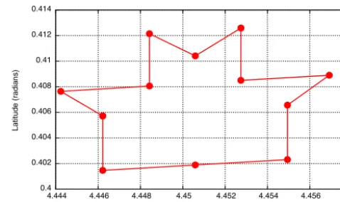
Figure 4. An example of a non-convex control volume in variable-resolution CAM-SE. Vertices are filled circles and they are con-nected with straight lines.
The set of indices for which center points of regular latitude–longitude grid cells are located in gnomonic cubed-sphere cellAi is denotedSi. Note that, since the raw data
sets are higher resolution, the cubed-sphereSi is guaranteed
to be non-empty. Through this binning process the approxi-mate average elevation in cubed-sphere cellibecomes
h(Acube)
i =
1
1Ai
X
j∈Si
h(0raw)
j 13j. (16)
Whenh(Acube)
i is known we can compute the sub-grid
vari-ance on the intermediate cubed-sphere gridA: Var(Atms)
i =
1
1Ai
X
j∈Si
h(Acube)
i −h
(raw) 0j
2
13j. (17)
The land fraction is also binned to the intermediate cubed-sphere grid,
f(Acube)
i =
1
1Ai
X
j∈Si
f0(raw)
j 13j. (18)
To remain consistent with previous GTOPO30-based to-pography generation software for CAM, all land fractions south of 79◦S are set to 1 for topography data based on GTOPO30, which effectively extends the land for the Ross Ice Shelf. There are eight types of masks in the MODIS data: shallow ocean, land, shoreline, shallow inland water, ephemeral water, deep inland water, moderate ocean, and deep ocean. Here we set all masks to 0 except land, shore-line and ephemeral water, which are set to 1. For topography data based on MODIS, no further alternations are made to the land fraction.
k
A
lΩ
Ω
kl
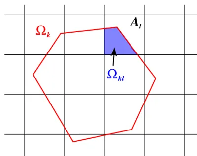
Figure 5. Schematic of the notation used to define the overlap be-tween target grid cellk(red polygon) and high-resolution cubed-sphere grid cellA`(Cartesian-like grid in figure). The overlap area,
k`=k∩A`, is shaded with a cross-hatch pattern in the figure.
cubed-sphere grid using the geometrically exact algorithm of Ullrich et al. (2009) optimized for the regular latitude– longitude and gnomonic cubed-sphere grid pair or the more general remapping algorithms such as SCRIP (Jones, 1999) and Kritsikis et al. (2015).
2.2.2 Step 2: cubed-sphere grid to target grid (A→) The cell-averaged values of elevation and sub-grid-scale variances (Var(tms)and Var(gwd)) on the target grid are com-puted by rigorously remapping the variables from the cubed-sphere grid to the target grid. As for step 1 of the algorithm, several methods could be used such as SCRIP and Kritsikis et al. (2015). The latter has the advantage of more accurately representing both small- and great-circle arc sides of the con-trol volumes, whereas SCRIP approximates cells’ sides in latitude–longitude space. Here the remapping is performed using CSLAM (Conservative Semi-LAgrangian Multi-tracer transport scheme) technology (Lauritzen et al., 2010), which approximates the cell sides with great-circle arcs. That said, the algorithm can still operate on grids where the control volumes do not consist of great-circle arcs, such as regu-lar latitude–longitude grids where the control volume sides parallel with latitudes are small-circle arcs, but there will be an additional truncation error in the geometric approx-imation to the control volumes. It is possible to use large parts of the CSLAM technology since the source grid is a gnomonic cubed-sphere grid; hence, instead of remapping between the gnomonic cubed-sphere grid and a deformed La-grangian grid, as done in CSLAM transport, the remapping is from the gnomonic cubed-sphere grid to any target grid constructed from great-circle arcs (the target grid “plays the role” of the Lagrangian grid). However, a couple of modifica-tions were made to the CSLAM search algorithm. First of all, the target grid cells can have an arbitrary number of vertices,
whereas the CSLAM transport search algorithm assumes that the target grid consists of quadrilaterals and the number of overlap areas is determined by the deformation of the trans-porting velocity field. In the case of the remapping needed in this application, the target grid consists of polygons with any number of vertices and the search is not constrained by the physical relation between regular and deformed upstream quadrilaterals. Secondly, the CSLAM search algorithm for transport assumes that the target grid cells are convex, which is not necessarily the case for target grids. The CSLAM search algorithm has been modified to support non-convex cells that are, for example, encountered in variable-resolution CAM-SE (see Fig. 4); essentially that means that any tar-get grid cell may cross a gnonomic isoline (source grid line) more than twice.
Let the target grid consist ofNtgrid cellsk,k=1, . . ., Nt with associated spherical area 1k. The search algorithm
for CSLAM is used to identify overlap areas between the target grid cellk and the cubed-sphere grid cellsA`,`=
1, . . ., Nc. Denote the overlap area betweenkandA`
k`=k∩A`, (19)
(see Fig. 5) and letLk denote the set of indices for which k∩A`,`=1, . . ., Ncis non-empty.
Note that the computation of overlap areask` is
facil-itated by the “Cartesian” layout of the equiangular cubed-sphere grid in computational space. The target grid vertex locations within the cubed-sphere source grid are computed by first locating which panel the vertices are on (using the “coordinate maximality” algorithm Eq. 13), and their loca-tions thereafter trivially result when the vertex coordinates are converted into the particular panels equiangular coor-dinates (Eqs. 14 and 15). The overlap areas are computed by finding intersection between the(x, y)gnomonic isolines (“Cartesian” layout) and the target grid cell sides. Since topo-graphic variables are computed just once for each horizontal grid resolution, computational performance is less critical. On a standard laptop even high-resolution (e.g., 25 km) grid overlaps are computed on the order of minutes irrespective of the target grid topology (Voronoi, cubed sphere, etc.).
The average elevation and variance used for TMS in target grid cellkare respectively given by
h(tgt,raw)
k =
1
1k
X
`∈Lk
h(Acube)
` 1k`, (20)
Var(tms)
k =
1
1k
X
`∈Lk
Var(tms)
` 1k`. (21)
The variance of the cubed-sphere datah(cube)with respect to the target grid cell average valuesh(tgt,raw)is given by Var(gwd,raw)
k =
1
1k
X
`∈Lk
h(tgt,raw)
k −h
(cube) A`
2
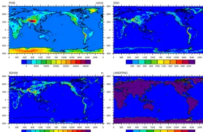
Figure 6. Surface geopotential8s(upper left), SGH (upper right), SGH30 (lower left) and LANDFRAC (lower right) for CAM-SE NE30NP4
resolution (“16×” smoothing)). The data are plotted on the native grid. NCL scripts to create this figure are released with the software source code.
The appended superscript “raw” in h(tgt,raw) and Var(gwd,raw) refers to the fact that the elevation and GWD variance is based on unsmoothed elevation. As mentioned in the Introduction, the elevation (for models based on terrain-following coordinates) is usually smoothed – i.e., the highest wave numbers are removed. This smoothed elevation is denotedh(tgt,smooth).
After smoothing the target grid elevation, the sub-grid-scale variance for GWD could be recomputed as the smooth-ing operation will add energy to the smallest wavelengths: Var(gwd,smooth)
k =
1
1k
X
`∈Lk
h(tgtk,smooth)−h(Acube` )
2
1k`. (23)
See discussion on the difference between using Var(gwd,raw) or h(tgt,smooth) in Sect. 3. The smoothing of elevation is discussed in some detail in the next section. 2.2.3 Smoothing of elevationh(tgt)(if applicable) As discussed in the Introduction, mapping the elevation to the target grid without further filtering to remove the high-est wave numbers usually leads to excessive spurious noise in the simulations when using terrain-following coordinates. Non-terrain-following coordinates such as theηcoordinates (Mesinger, 1984; Mesinger et al., 1988) and zcoordinates
using shaved cells or cut cells (Adcroft et al., 1997; Walko and Avissar, 2008) do not require filtering of topography. For models that do require topography smoothing, there seems to be no standardized procedure, for example a test case suite, to objectively select the level of smoothing and the filtering method. The amount of smoothing necessary to remove spu-rious noise in, for example, vertical velocity depends on the amount of inherent or explicit numerical diffusion in the dy-namical core (e.g., Lauritzen et al., 2011). It may be consid-ered important that the topographic smoothing is done with discrete operators consistent with the dynamical core.
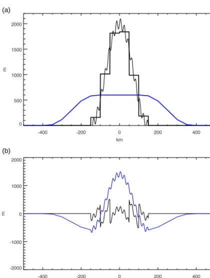
(a)
(b)
Figure 7. (a) Idealized topography 1000+1000·cos(2π·x/300)+ 100·sin(2π/20)for−150 km< x <150 km (thin black line), pography averaged in 50 km grid boxes (thick black line), and to-pography smoothed with boxcar smoother using a 500 km window (thick blue line). (b) Deviation of topography from 50 km grid-box mean (thin black line), and deviations from 500 km grid- boxcar-smoothed topography (thin blue line).
heights while filtering out small scales: envelope topography adjusts the surface height with sub-grid-scale topographic variance (Wallace et al., 1983; Mesinger and Strickler, 1982). Loosely speaking, the otherwise smoothed peak heights are raised. This process may perturb the average surface height. Alternatively, one may use silhouette averaging (Smart et al., 2005; Walko and Tremback, 2004; Bossert, 1990). A similar approach, but implemented as variational filtering, is taken in Rutt et al. (2006); this method also imposes additional con-straints such as enforcing zero elevation over ocean masks.
As there is no standard procedure for smoothing raphy, we leave it up to the user to smooth the raw topog-raphy h(tgt,raw). The smoothed topography is referred to as
h(tgt,smooth).
Figure 8. Difference between
√
Var(gwd,smooth)and √
Var(gwd,raw) for CAM-SE NE30NP4, where the smoothed PHIS is the “16×” configuration.
2.3 Naming conventions
The naming conventions for the topographic variables in the software and NetCDF files are as follows:
PHIS=g h(tgt), (24)
SGH= q
Var(gwd), (25)
SGH30= q
Var(tms), (26)
LANDFRAC=f(tgt), (27)
wheregis the gravitational constant.
3 Results
Below the topography software has been applied to different dynamical core grids in CAM, for example CAM-SE, which uses the spectral element dynamical core from HOMME (High-Order Method Modeling Environment; Thomas and Loft, 2005; Dennis et al., 2005), as well as FV. CAM-SE is defined on a cubed-sphere grid, and we show results for a configuration of approximately 1◦resolution, which is the NE30NP4 setup with 30×30 elements on each cubed-sphere panel and 4×4 Gauss–Lobatto–Legendre (GLL) quadrature points in each element. CAM-FV topography data are shown for the 0.9◦×1.25◦resolution. The topography software has
Height
Figure 9. The difference between GMTED2010 and GTOPO30 (left) elevation (in m) and (right) SGH30 (in m), respectively, on the inter-mediate 3 km cubed-sphere grid.
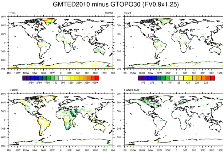
Figure 10. The difference between GMTED2010 and GTOPO30 topographic variables for CAM-FV at approximately 1◦resolution.
3.1 Example: smoothing methods used in CAM-FV and CAM-SE
As mentioned in Sect. 2.2.3 dynamical cores may need smoothing of elevation data. In the CAM-FV the highest wave numbers are removed by mapping8s (surface geopo-tential) to a regular latitude–longitude grid that is half the resolution of the desired model resolution and then mapping back to the model grid by one-dimensional remaps along lat-itudes and longlat-itudes, respectively, using the PPM (piece-wise parabolic method) with monotone filtering. In CAM-SE the surface geopotential is smoothed by multiple appli-cations of the CAM-SE Laplace operator combined with a bound-preserving limiter. Figure 2 shows different levels of smoothing of surface height for CAM-SE and, for
compari-son, CAM-FV. It can clearly be seen that there are large dif-ferences between the height of the mountains with different smoothing operators and smoothing strength. Figure 6 shows the topography variables for CAM-SE based on GTOPO30 raw data and smoothing with 16 applications of the Laplace operator.
3.2 Topography smoothing and SGH
a parameterization scheme represents the drag and other ef-fects induced by waves forced by “unresolved” topographic deviations (thin black line, Fig. 7b). The grid mean of these deviations is zero.
However, when additional smoothing is applied to the grid-box mean topography (thick blue line, Fig. 7a), the situ-ation becomes less well defined. It is difficult to argue that the “unresolved” topographic forcing is fully captured by the de-viations from the grid-box mean. On the other hand, the devi-ations from the smoothed topography (thin blue line, Fig. 7b) have properties that make it unclear how to incorporate them in a traditional gravity wave parameterization framework. The grid-box mean of these deviations is not zero. Non-zero deviations can exist far from actual topographic forcing. In the case of real-world topography, Fig. 8 shows the differ-ence between
√
Var(gwd,smooth)and √
Var(gwd,raw). There are significant differences between SGH based on smoothed or unsmoothed topography. We do not advocate any particular strategy for parameterization of sub-grid orographic effects; our software is simply intended to make the generation of the forcing data sets for global models traceable and transparent. 3.3 GTOPO30 and GMTED2010 raw data
Many global models use GTOPO30 as the raw topography data; however, more accurate data sets are available, such as GMTED2010. NCAR_Topo (v1.0) is set up to use both GTOPO30 and GMTED2010 (with MODIS for land frac-tion) source data. The differences between the raw 1 km data sets are discussed in detail in Danielson and Gesch (2011). Here we focus on the differences between the data sets on the approximately 3 km cubed-sphere grid and standard cli-mate model resolutions (approxicli-mately 100 km). Figure 9 shows the elevation differences as well as SGH30 differences on the intermediate (approximately 3 km) cubed-sphere grid. There are significant differences in elevation, especially over Greenland, Antarctica and South America, as well as associ-ated changes to SGH30. Even at the 100 km scale and with topography smoothing, the differences are rather large (see Fig. 10). The differences in land fraction are mainly due to MODIS providing a more detailed land–water mask. There are eight types of masks in the MODIS data: shallow ocean, land, shoreline, shallow inland water, ephemeral water, deep inland water, moderate ocean, and deep ocean. Here we set all masks to 0 except land, shoreline and ephemeral water, which are set to 1.
4 Conclusions
The NCAR global model topography generation software for unstructured grids (NCAR_Topo (v1.0)) has been doc-umented and example applications to CAM have been pre-sented. The topography software computes sub-grid-scale variances using a quasi-isotropic separation of scales through
the intermediate mapping of high-resolution elevation data to an equiangular cubed-sphere grid. The software supports structured or unstructured (e.g., variable resolution) global grids.
Code availability
The source codes for the NCAR Global Model Topography Generation Software for Unstructured Grids are available through GitHub. The repository URL is https://github.com/ UCAR/Topo/tags/. The repository also contains NCL scripts to plot the topography variables (Fig. 6) that the software generates.
Acknowledgements. NCAR is sponsored by the National Science
Foundation (NSF). M. Taylor was supported by the Department of Energy Office of Biological and Environmental Research, work package 12-015334 “Multiscale Methods for Accurate, Efficient, and Scale-Aware Models of the Earth System”. Thanks to Sang-hun Park (NCAR) for providing data for the GTOPO30 power spectrum. Thanks to Max Suarez (NASA) for encouraging upgrading to the GMTED2010 data. We thank the two reviewers for their useful comments. Partial support for this work was provided through the Scientific Discovery through Advanced Computing (SciDAC) program funded by U.S. Department of Energy, Office of Science, Advanced Scientific Computing Research.
Edited by: S. Valcke
References
Adcroft, A., Hill, C., and Marshall, J.: Representation of Topog-raphy by Shaved Cells in a Height Coordinate Ocean, Mon. Weather Rev., 125, 2293–2315, 1997.
Bacmeister, J.: Mountain-wave drag in the stratosphere and meso-sphere inferred from observed winds and a simple mountain-wave parameterization scheme, J. Atmos. Sci., 50, 377–399, doi:10.1175/1520-0469(1993)050<0377:MWDITS>2.0.CO;2, 1993.
Baines, P. and Palmer, T.: Rationale for a new physically based parametrization of subgrid-scale orographic effects, ECMWF Tech. Memo., 1699, 1990.
Balmino, G.: The Spectra of the topography of the Earth, Venus and Mars, Geophys. Res. Lett., 20, 1063–1066, doi:10.1029/93GL01214, 1993.
Beljaars, A., Brown, A., and Wood, N.: A new parametrization of turbulent orographic form drag, Q. J. Roy. Meteorol. Soc., 130, 1327–1347, doi:10.1256/qj.03.73, 2004.
Bénard, P.: An assessment of global forecast errors due to the spher-ical geopotential approximation in the shallow-water case, Q. J. Roy. Meteorol. Soc., 141, 195–206, doi:10.1002/qj.2349, 2015. Bossert, J. E.: Regional-scale flow in complex terrain: An
Bougeault, P., Clar, A. J., Benech, B., Carissimo, B., Pelon, J., and Richard, E.: Momentum Budget over the Pyrénées: The PYREX Experiment, B. Am. Meteorol. Soc., 71, 806–818, 1990. Danielson, J. and Gesch, D.: Global Multi-resolution Terrain
Eleva-tion Data 2010 (GMTED2010), Open-file report 2011-1073, US Geological Survey, available at: http://pubs.usgs.gov/of/2011/ 1073/pdf/of2011-1073.pdf, 2011.
Dennis, Fournier, A., Spotz, W. F., St-Cyr, A., Taylor, M. A., Thomas, S. J., and Tufo, H.: High-Resolution Mesh Convergence Properties and Parallel Efficiency of a Spectral Element Atmo-spheric Dynamical Core, Int. J. High Perform. Comput. Appl., 19, 225–235, doi:10.1177/1094342005056108, 2005.
Durran, D.: Lee waves and mountain waves, in: Encyclopedia of Atmospheric Sciences, edited by: Holton, J. R., Academic Press, London, UK, 1161–1169, doi:10.1016/B0-12-227090-8/00202-5, 2003.
Durran, D.: Numerical Methods for Fluid Dynamics: With Applica-tions to Geophysics, vol. 32 of Texts in Applied Mathematics, 2 edn., Springer, New York, USA, 516 pp., 2010.
Eckermann, Y. K. S. and Chun, H.-Y.: An overview of the past, present and future of gravity-wave drag parametrization for nu-merical climate and weather prediction models: survey article, Atmos. Ocean, 41, 65–98, doi:10.3137/ao.410105, 2003. ECMWF: Proceedings of a workshop on orography, ECMWF,
Reading, UK, 1997.
Farr, T. G., Rosen, P. A., Caro, E., Crippen, R., Duren, R., Hens-ley, S., Kobrick, M., Paller, M., Rodriguez, E., Roth, L., Seal, D., Shaffer, S., Shimada, J., Umland, J., Werner, M., Oskin, M., Burbank, D., and Alsdorf, D.: The Shuttle Radar Topography Mission, Rev. Geophys., 45, 1–33, doi:10.1029/2005RG000183, 2007.
Gagnon, J.-S., Lovejoy, S., and Schertzer, D.: Multifractal earth topography, Nonlin. Processes Geophys., 13, 541-570, doi:10.5194/npg-13-541-2006, 2006.
Gates, W.: Derivation of the Equations of Atmospheric Motion in Oblate Spheroidal Coordinates, J. Atmos. Sci., 61, 2478–2487, doi:10.1175/1520-0469(2004)061<2478:DOTEOA>2.0.CO;2, 2004.
Gesch, D. B. and Larson, K. S.: Techniques for development of global 1-kilometer digital elevation models, in: Pecora Thirteenth Symposium, Am. Soc. Photogrammetry Remote Sens., Soiux Falls, South Dakota, 1998.
GLOBE Task Team and others: The Global Land One-kilometer Base Elevation (GLOBE) Digital Elevation Model, Version 1.0, available at: http://www.ngdc.noaa.gov/mgg/topo/globe. html (last access: 18 June 2015), 1999.
Jones, P. W.: First- and Second-Order Conservative Remapping Schemes for Grids in Spherical Coordinates, Mon. Weather Rev., 127, 2204–2210, 1999.
Kim, Y.-J. and Doyle, J. D.: Extension of an orographic-drag parametrization scheme to incorporate orographic anisotropy and flow blocking, Q. J. Roy. Meteorol. Soc., 131, 1893–1921, doi:10.1256/qj.04.160, 2005.
Kritsikis, E., Aechtner, M., Meurdesoif, Y., and Dubos, T.: Conser-vative interpolation between general spherical meshes, Geosci. Model Dev. Discuss., 8, 4979–4996, doi:10.5194/gmdd-8-4979-2015, 2015.
Lander, J. and Hoskins, B.: Believable scales and parameterizations in a spectral transform model, Mon. Weather Rev., 125, 292–303,
doi:10.1175/1520-0493(1997)125<0292:BSAPIA>2.0.CO;2, 1997.
Lauritzen, P. H. and Nair, R. D.: Monotone and conservative Cascade Remapping between Spherical grids (CaRS): Regular latitude-longitude and cubed-sphere grids, Mon. Weather Rev., 136, 1416–1432, 2008.
Lauritzen, P. H., Nair, R. D., and Ullrich, P. A.: A conserva-tive semi-Lagrangian multi-tracer transport scheme (CSLAM) on the cubed-sphere grid, J. Comput. Phys., 229, 1401–1424, doi:10.1016/j.jcp.2009.10.036, 2010.
Lauritzen, P. H., Mirin, A., Truesdale, J., Raeder, K., Ander-son, J., Bacmeister, J., and Neale, R. B.: Implementation of new diffusion/filtering operators in the CAM-FV dynam-ical core, Int. J. High Perform. Comput. Appl., 26, 63–73, doi:10.1177/1094342011410088, 2011.
Lin, S.-J.: A ’Vertically Lagrangian’ Finite-Volume Dynamical Core for Global Models, Mon. Weather Rev., 132, 2293–2307, 2004.
Lott, F.: Alleviation of Stationary Biases in a GCM through a Moun-tain Drag Parameterization Scheme and a Simple Representa-tion of Mountain Lift Forces, Mon. Weather Rev., 127, 788–801, doi:10.1175/1520-0493(1999)127, 1999.
Lott, F. and Miller, M. J.: A new subgrid-scale orographic drag parametrization: Its formulation and testing, Q. J. Roy. Meteo-rol. Soc., 123, 101–127, doi:10.1002/qj.49712353704, 1997. Monaghan, A. J., Barlage, M., Boehnert, J., Phillips, C. L., and
Wil-helmi, O. V.: Overlapping interests: the impact of geographic co-ordinate assumptions on limited-area atmospheric model simula-tions, Mon. Weather Rev., 141, 2120–2127, doi:10.1175/MWR-D-12-00351.1, 2013.
Mesinger, F.: A blocking technique for representation of mountains in atmospheric models, Rivista di Meteorologia Aeronautica, 44, 195–202, 1984.
Mesinger, F. and Strickler, R. F.: Effect of Mountains on Genoa Cyclogeneses, J. Meteorol. Soc. Jpn., 60, 326–337, 1982. Mesinger, F., Janji´c, Z., Niˇckovi´c, S., Gavrilov, D., and Deaven,
D. G.: The Step-Mountain Coordinate: Model Description and Performance for Cases of Alpine Lee Cyclogenesis and for a Case of an Appalachian Redevelopment, Mon. Weather Rev., 116, 1493–1518, doi:10.1175/1520-0493(1988)116, 1988. Nair, R. D., Thomas, S. J., and Loft, R. D.: A Discontinuous
Galerkin Transport Scheme on the Cubed Sphere, Mon. Weather Rev., 133, 814–828, 2005.
Navarra, A., Stern, W. F., and Miyakoda, K.: Reduction of the Gibbs Oscillation in Spectral Model Simulations, J. Climate, 7, 1169– 1183, 1994.
Neale, R. B., Chen, C.-C., Gettelman, A., Lauritzen, P. H., Park, S., Williamson, D. L., Conley, A. J., Garcia, R., Kinnison, D., Lamarque, J.-F., Marsh, D., Mills, M., Smith, A. K., Tilmes, S., Vitt, F., Cameron-Smith, P., Collins, W. D., Iacono, M. J., Easter, R. C., Ghan, S. J., Liu, X., Rasch, P. J., and Taylor, M. A.: De-scription of the NCAR Community Atmosphere Model (CAM 5.0), NCAR Technical Note, National Center of Atmospheric Re-search, Boulder, Colorado, USA, 2010.
Rutt, I., Thuburn, J., and Staniforth, A.: A variational method for orographic filtering in NWP and climate models, Q. J. Roy. Me-teorol. Soc., 132, 1795–1813, doi:10.1256/qj.05.133, 2006. Scinocca, J. and McFarlane, N.: The parametrization of drag
in-duced by stratified flow over anisotropic orography, Q. J. Roy. Meteorol. Soc., 126, 2353–2393, doi:10.1002/qj.49712656802, 2000.
Skamarock, W. C., Klemp, J. B., Duda, M. G., Fowler, L., Park, S.-H., and Ringler, T. D.: A Multi-scale Nonhydro-static Atmospheric Model Using Centroidal Voronoi Tesselations and C-Grid Staggering, Mon. Weather Rev., 240, 3090–3105, doi:10.1175/MWR-D-11-00215.1, 2012.
Smart, J., Shaw, B., and McCaslin, P.: WRF SI V2.0: Nest-ing and details of terrain processNest-ing, 13, available at: http:// www.wrf-model.org/si/WRFSI-V2.0-Nesting-Ter-Proc.pdf (last access: 18 June 2015), 2005.
Staniforth, A. and White, A.: Geophysically Realistic, Ellipsoidal, Analytically Tractable (GREAT) coordinates for atmospheric and oceanic modelling, Quart. J. Roy. Meteorol. Soc., 141, 1646– 1657, doi:10.1002/qj.2467, 2015.
Thomas, S. J. and Loft, R. D.: The NCAR Spectral Element Cli-mate Dynamical Core: Semi-Implicit Eulerian Formulation, J. Sci. Comput., 25, 307–322, 2005.
Uhrner, U.: The impact of new sub-grid scale orography fields on the ECMWF model, ECMWF Tech. Memo., 329, 2001.
Ullrich, P. A., Lauritzen, P. H., and Jablonowski, C.: Geometrically Exact Conservative Remapping (GECoRe): Regular latitude-longitude and cubed-sphere grids, Mon. Weather Rev., 137, 1721–1741, 2009.
Walko, R. and Tremback, C. J.: RAMS, Regional Atmospheric Modeling System, Version 4.3/4.4, Model Input Namelist Param-eters, Boulder, Colorado, USA, 2004.
Walko, R. L. and Avissar, R.: The Ocean-Land-Atmosphere Model (OLAM). Part II: Formulation and Tests of the Nonhydro-static Dynamic Core, Mon. Weather Rev., 136, 4045–4062, doi:10.1175/2008MWR2523.1, 2008.
Wallace, J. M., Tibaldi, S., and Simmons, A. J.: Reduction of sys-tematic forecast errors in the ECMWF model through the intro-duction of an envelope orography, Q. J. Roy. Meteorol. Soc., 109, 683–717, doi:10.1002/qj.49710946202, 1983.
Webster, S., Brown, A. R., Cameron, D. R., and Jones, P. C.: Im-provements to the representation of orography in the Met Office Unified Model, Q. J. Roy. Meteorol. Soc., 129, 1989–2010, 2003. White, A. A., Staniforth, A., and Wood, N.: Spheroidal coordinate systems for modelling global atmospheres, Q. J. Roy. Meteorol. Soc., 134, 261–270, 2008.