www.geosci-model-dev.net/5/111/2012/ doi:10.5194/gmd-5-111-2012
© Author(s) 2012. CC Attribution 3.0 License.
Geoscientific
Model Development
The 1-way on-line coupled atmospheric chemistry model system
MECO(n) – Part 2: On-line coupling with the Multi-Model-Driver
(MMD)
A. Kerkweg1and P. J¨ockel2
1Institute for Atmospheric Physics, University of Mainz, 55099 Mainz, Germany
2Deutsches Zentrum f¨ur Luft- und Raumfahrt (DLR), Institut f¨ur Physik der Atmosph¨are, 82234 Oberpfaffenhofen, Germany Correspondence to: A. Kerkweg ([email protected])
Received: 23 May 2011 – Published in Geosci. Model Dev. Discuss.: 21 June 2011 Revised: 10 January 2012 – Accepted: 11 January 2012 – Published: 19 January 2012
Abstract. A new, highly flexible model system for the seam-less dynamical down-scaling of meteorological and chem-ical processes from the global to the meso-γ scale is pre-sented. A global model and a cascade of an arbitrary num-ber of limited-area model instances run concurrently in the same parallel environment, in which the coarser grained stances provide the boundary data for the finer grained in-stances. Thus, disk-space intensive and time consuming intermediate and pre-processing steps are entirely avoided and the time interpolation errors of common off-line nesting approaches are minimised. More specifically, the regional model COSMO of the German Weather Service (DWD) is nested on-line into the atmospheric general circulation model ECHAM5 within the Modular Earth Submodel Sys-tem (MESSy) framework. ECHAM5 and COSMO have pre-viously been equipped with the MESSy infrastructure, im-plying that the same process formulations (MESSy submod-els) are available for both models. This guarantees the high-est degree of achievable consistency, between both, the mete-orological and chemical conditions at the domain boundaries of the nested limited-area model, and between the process formulations on all scales.
The on-line nesting of the different models is estab-lished by a client-server approach with the newly developed Multi-Model-Driver (MMD), an additional component of the MESSy infrastructure. With MMD an arbitrary number of model instances can be run concurrently within the same message passing interface (MPI) environment, the respec-tive coarser model (either global or regional) is the server for the nested finer (regional) client model, i.e. it provides the data required to calculate the initial and boundary fields to the client model. On-line nesting means that the coupled (client-server) models exchange their data via the computer
memory, in contrast to the data exchange via files on disk in common off-line nesting approaches. MMD consists of a li-brary (Fortran95 and some parts in C) which is based on the MPI standard and two new MESSy submodels, MMDSERV and MMDCLNT (both Fortran95) for the server and client models, respectively.
MMDCLNT contains a further sub-submodel, INT2COSMO, for the interpolation of the coarse grid data provided by the server models (either ECHAM5/MESSy or COSMO/MESSy) to the grid of the respective client model (COSMO/MESSy). INT2COSMO is based on the off-line pre-processing tool INT2LM provided by the DWD.
The new achievements allow the setup of model cascades for zooming (down-scaling) from the global scale to the lower edge of the meso-γ scale (≈1 km) with a very high degree of consistency between the different models and be-tween the chemical and meteorological boundary conditions.
1 Introduction
The quality of the results of a regional (or limited-area) at-mospheric model are highly influenced by the conditions pre-scribed at the model domain boundaries.
For the meteorological/dynamical state of limited-area models, these boundary conditions are usually prescribed from analysis, reanalysis or forecast data from global or re-gional numerical weather prediction models or from global climate models, the so-called driving models1. Technically, 1Appendix B contains a glossary explaining some terms
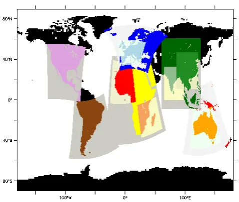
Fig. 1. Example for a MECO(n) model cascade setup using 13
in-stances (1 ECHAM/MESSy,n=12 COSMO/MESSy instances).
the boundary data is read from specifically pre-processed data files stored on disk with a typical time resolution of 1– 6 h, depending on the driving model.
Including processes for atmospheric chemistry in limited-area models forms a particular challenge in this respect, mainly because the amount of prognostic variables increases drastically. First, the chemical constituents need to be in-cluded, and second a higher update frequency for the chem-ical boundary conditions is desirable in order to be able to resolve the diurnal changes. In addition, it is favourable to describe the chemical processes in the limited-area model as consistent as possible with those in the driving model.
These requirements render the off-line coupling, where data are exchanged via the disk system, unfeasible. We therefore propose an on-line coupling approach, where the driving model and the limited-area model run concurrently in the same MPI environment and directly exchange the fields required to calculate the initial and boundary condi-tions via the computer memory. Figure 1 gives an exam-ple for such a model setup, showing 13 model instances run-ning concurrently: one global instance (ECHAM5/MESSy) drives six COSMO/MESSy instances directly. Two of these COSMO/MESSy instances (covering Europe and Australia) drive again one further smaller scale COSMO/MESSy in-stance each, two more COSMO/MESSy inin-stances (cover-ing Asia and Africa) drive two further COSMO/MESSy in-stances each. All these inin-stances are running simultaneously using the newly developed system. To abbreviate the naming we call this system MECO(n), “MESSy-fied ECHAM and COSMO nested n times”.
The outline of this document is as follows: first, we de-scribe the applied model components (Sect. 2) and provide details about the implementation of the on-line coupling
(Sect. 3). In Sect. 4 we classify our coupling approach in comparison to other coupling approaches used in Earth sys-tem modeling. Section 5 explains the few adjustments of namelist and run-script entries, which are required to run a model cascade. The Multi-Model-Driver (MMD) library, performing the data exchange between the concurrently run-ning models, is described briefly in Sect. 6. The “MMD li-brary manual”, which is part of the Supplement, comprises a detailed description of the library routines. Sections 7 and 8 sketch the work flow of the server submodel MMDSERV and the client submodel MMDCLNT, organizing the coupling on the server and the client side, respectively. Section 9 explains some technical details about the implementation of the on-line coupling into COSMO/MESSy and of the stand-alone program INT2LM as MESSy sub-submodel INT2COSMO2. Some remarks on how to achieve the optimum run-time per-formance efficiency with MECO(n) are provided in Sect. 10, and in Sect. 11 we close with a summary and an outlook. Ex-ample applications are presented in the companion articles (Kerkweg and J¨ockel, 2012; Hofmann et al., 2012).
2 Applied model components
This new approach is based on the Modular Earth Submodel System (MESSy, J¨ockel et al., 2005, 2010). MESSy provides a variety of process parameterisations coded as independent submodels, e.g. for gas-phase chemistry (MECCA, Sander et al., 2005), for scavenging of trace gases (SCAV, Tost et al., 2006), convective tracer transport (CVTRANS, Tost et al., 2010), etc. Furthermore, MESSy provides the interface to couple these submodels to a basemodel via a highly flexible data management facility.
MESSy has been connected to the global climate model ECHAM5 (Roeckner et al., 1996) extending it to the at-mospheric chemistry general circulation model (AC-GCM) ECHAM5/MESSy (J¨ockel et al., 2006, 2010). Further-more, MESSy was connected to the non-hydrostatic limited-area weather prediction model of the Consortium for Small-Scale Modelling (COSMO, previously called “Lokal-Model” (LM), Steppeler et al., 2003; Doms and Sch¨attler, 1999) resulting in the regional atmospheric chemistry model COSMO/MESSy (Kerkweg and J¨ockel, 2012). Therefore, all processes included in MESSy and used in both mod-els are described consistently on the global and the regional scale, if ECHAM5/MESSy is used as driving model for COSMO/MESSy.
During the last years, the numerical weather prediction model COSMO was further developed to fulfil the require-ments for a regional climate model by the Climate Limited-area Modelling (CLM)-community (see Rockel et al., 2008). These developments also include the expansion of the stand-alone program INT2LM, which is provided by the German 2The “MMD user manual”, which is also part of the
COSMO/MESSy model MMDCLNT ECHAM5/MESSy ECHAM5
DATA file
PREPROCESSOR
DATA file
INT2LM
DATA file
COSMO model
MMDSERV
INT2COSMO
M
M
D
on
li
ne
d
at
a
tra
ns
fe
r
DATA preprocessing
for COSMO model Online coupledCOSMO/MESSy
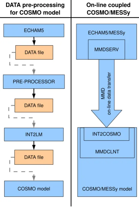
Fig. 2. Comparison of the data (pre-)processing procedure
pro-viding boundary data for one time step to one instance of the stand-alone COSMO model (left) and of the on-line coupled COSMO/MESSy model using ECHAM5/MESSy as driving model (right). The stand-alone COSMO model requires four indepen-dent sequential tasks. First, the driving model ECHAM5 is run. Second, the output files of ECHAM5 are used as input to a pre-processing tool converting the ECHAM5 data to a format readable by INT2LM. Third, the pre-processor INT2LM calculates and out-puts the initial and boundary files for the COSMO model, which, fourth, is run to perform the intended simulation. In the on-line cou-pled model system the input data required for the COSMO model is exchanged on-line via the MMD library and interpolated on-line in the MESSy sub-submodel INT2COSMO. Thus no intermediate manual data processing is required.
Weather Service (DWD) for the pre-processing of the ini-tial and boundary data for the COSMO model: the original INT2LM as provided by DWD can process data from three different driving models:
– the global DWD grid point model on an icosahedral grid (GME),
– the global spectral model IFS of ECMWF and
– the regional COSMO model, as the COSMO model can be nested (so far off-line) into itself.
In addition to the standard driving models supported by the DWD, the INT2LM was further developed by the CLM-Community to also interpolate data of climate models (e.g. ECHAM or REMO) and other weather prediction models. In case of ECHAM an additional pre-processing procedure is required to transform the standard output data of the cli-mate model into a uniform format which can be handled by INT2LM.
The left-hand side of Fig. 2 depicts a common pre-processing procedure for producing the initial and bound-ary data with the stand-alone INT2LM for one time step of the COSMO model: first, the global model (here ECHAM5) is run. Afterwards, the output of ECHAM5 needs to be pre-processed to be readable for INT2LM. Subsequently, INT2LM is run and initial and boundary data for the COSMO model are produced. Finally, the simulation with the COSMO model is performed.
If this pre-processing procedure is not only performed for the dynamical part of the model, but also for the chemical part, the pre-processing time and the required data storage increase enormously, as chemical setups re-quire boundary data for most chemical tracers taken into account. State-of-the-art atmospheric chemistry mecha-nisms typically consist of about 50 to a few hundred trac-ers. Furthermore, to capture the diurnal variations, the coupling frequency is higher for atmospheric chemistry simulations. To avoid the increasing effort for the pre-processing and the additional data, we implemented the on-line coupling of ECHAM5/MESSy to COSMO/MESSy and of COSMO/MESSy to COSMO/MESSy into MESSy. This is sketched on the right-hand side of Fig. 2. Cur-rently, the on-line coupled model system is based on the ECHAM model version 5.3.02, the COSMO model version cosmo_4.8_clm12and MESSy version 2.41.
3 Coupling procedure
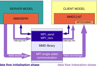
To carry out the on-line coupling, we extended MESSy by the Multi-Model-Driver (MMD) library and two MESSy sub-models (MMDSERV and MMDCLNT). Following a client-server approach, the client-server (driving model) provides the data to the client model, which subsequently calculates its own initial and boundary data. The MMD library manages the data exchange between the individual (parallel decomposed) tasks of the different model executables very efficiently, as the field exchange during the time integration is implemented as point-to-point, single-sided, non-blocking MPI communi-cation. Figure 3 sketches the role of the MMD library, which is based on the message passing interface (MPI) library.
CLIENT MODEL
SERVER MODEL
MMDCLNT
data flow integration phase
data flow initialisation phase
INT2COSMO
field exchange
MMDSERV
field exchange
interrupt info
MMD library
MPI single sided
communication
MPI_send
MPI_recv
interrupt info
Fig. 3. Data exchange between the different model components: during the initialisation phase information is exchanged via MPI direct
communication between the server and the client model (dark blue arrows). During the integration phase the server provides the in-fields to the client via MPI point-to-point single sided non-blocking communication (violet). The additional information, if the server is interrupted after the current time step (e.g. for restarts), is exchanged each server time step using MPI direct communication.
manages the data exchange for the server model. MMD-CLNT not only carries out the data exchange for the client, it also performs the interpolation of the data provided by the server to produce the initial and boundary data required by the COSMO model. The latter is accomplished by the implementation of the stand-alone pre-processing program INT2LM as MMDCLNT submodel INT2COSMO. Thus, the INT2LM routines are also used for the calculation of the initial and boundary data in our on-line coupling approach. Furthermore, MMDCLNT provides the framework to use the INT2LM interpolation routines to interpolate additional fields, e.g. the tracers for chemistry calculations.
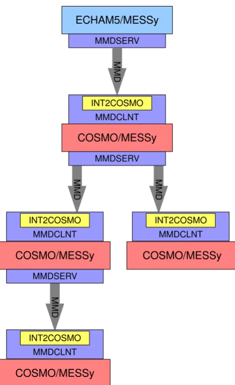
So far, we presented only one on-line coupled client-server pair. However, the MMD library provides the possibility to run an arbitrary number of models concurrently in the same MPI environment, which is only limited by the hard-ware capabilities. Thus a simulation setup is possible, in which one global model (i.e. ECHAM5/MESSy) is server for a number of COSMO/MESSy models. Each of the COSMO/MESSy models can again be server for a number of smaller scale COSMO/MESSy models and so forth (cf. Fig. 1). Thus, an entire cascade of on-line coupled mod-els can be run concurrently. Figure 4 illustrates an example layout for an on-line coupled MESSy model cascade. Fur-ther examples for a ECHAM5/MESSy→COSMO/MESSy
→COSMO/MESSy coupling are presented in the accompa-nying articles (Kerkweg and J¨ockel, 2012; Hofmann et al., 2012).
4 Discussion on the chosen coupling approach
In the Earth system modelling community the terms cou-pling3, coupler and coupled are widely used to describe a va-riety of aspects of connections within an Earth System Model (ESM), though rarely precised. In general, these terms are used to express some way of how different components in-fluence each other. Appendix A provides a detailed classifi-cation of coupling approaches.
The choice of the most suited coupling method depends on many aspects, not least on the desired application, but in summary a proper choice usually provides a compromise to minimise the computational and communication over-heads, the implementation effort (which depends mostly on the code structure of the involved legacy model(s)), and to maximise the desired degree of flexibility and sustainability. From the classification of operators (also in Appendix A), 3Note that the terms written in italics in this section do not refer
ECHAM5/MESSy
MMDSERV
COSMO/MESSy
COSMO/MESSy
COSMO/MESSy
MMD MMD
MMD
MMD
COSMO/MESSy
MMDSERV
MMDSERV
INT2COSMO MMDCLNT
INT2COSMO MMDCLNT
INT2COSMO MMDCLNT
INT2COSMO MMDCLNT
Fig. 4. Illustration of the data flow in an exemplary MECO(4) setup
with ECHAM5/MESSy as master Server and four COSMO/MESSy clients.
it is immediately clear that the internal coupling is the most widely used approach, since it is inherent to all Earth sys-tem models. J¨ockel et al. (2005) formalised this approach as process coupling by defining submodel implementations for process formulations (and diagnostics) and by defining an in-terface structure, which allows the strict separation of process implementations from shared model infrastructure (such as memory management, input/output, meta-data handling, call sequence etc.).
Examples for internal process coupling are the imple-mentation of atmospheric chemistry and/or the treatment of aerosols into an atmosphere model, as e.g. in COSMO-ART (Vogel et al., 2009), or the regular submodels of the Mod-ular Earth Submodel System (MESSy, J¨ockel et al., 2005), which have been coupled to ECHAM5 (J¨ockel et al., 2010) and COSMO (Kerkweg and J¨ockel, 2012) using the MESSy infrastructure.
For coupling operators on the domain level, examples for both, internal coupling and indirect external on-line cou-pling, exist. The Earth System Modeling Framework (ESMF, Collins et al., 2005) and the Community Climate System Model version 4 (CCSM4, Gent et al., 2011) use inter-nal coupling to allow for feedback between different do-main models. Pozzer et al. (2011) coupled the ocean model MPIOM (Jungclaus et al., 2006) to ECHAM/MESSy, and compared results and run-time performance to the indirectly, externally on-line coupled ECHAM5/MPIOM system (Jung-claus et al., 2006), which uses the OASIS3 coupler (Valcke et al., 2006). Other examples for external couplers are CPL6 (Craig et al., 2005) as employed in the Community Climate System Model 3 (Collins et al., 2006) and OASIS4 (Redler et al., 2010).
With MMD, we here provide a method which, in our clas-sification (Appendix A), provides a direct external on-line coupling method, i.e. avoiding the need of an additional ex-ternal coupler. The client – server approach of MMD com-prises two parts:
– The Multi-Model-Driver library provides a high-level API (application programming interface) for MPI based data exchange. The data transfer is implemented as single-sided, point-to-point communication, meaning that the data is sent from each server-task directly to the depending client tasks. The MMD library does not contain any rediscretisation facility. It is basemodel in-dependent and straightforwardly applicable for the cou-pling of other models.
– The server and client submodels MMDSERV and MMDCLNT, respectively, are basemodel dependent and need to be adapted to newly coupled models. In particular the client model, which includes the model specific interpolation routines (here in form of INT2COSMO) requires this adaption. Nevertheless, the basic structure of MMDCLNT and MMDSERV are ap-plicable to other models as well.
computationally more expensive) generalised transformation routines of a universal coupler.
5 Running the on-line coupled model system
Following the MESSy philosophy, setting up an on-line nested model cascade is as user-friendly as possible. In addi-tion to the usual setup of each model instance (which remains the same as for a single instance setup), the user needs to edit only the run-script and one namelist file per client-server pair:
– In the run-scriptxmessy_mmdthe model layout of the on-line coupled model cascade is defined. The user termines the number of model instances and the de-pendencies of the models, i.e. the client-server pairs. From this, the run-script generates the MMD namelist filemmd_layout.nml(see Sect. 6). Additionally, the file names and directories for the external data, required by INT2COSMO, have to be specified. A detailed ex-planation of the setup specific parts of the run-script are provided in the “MMD user manual” in the Supplement. – The MMDCLNT namelist file mmdclnt.nml con-tains all information required for the data exchange, i.e. the time interval for the data exchange and the fields that are to be provided by the server to the client. Section 8.1 explains the meaning of the individual namelist entries.
6 The Multi-Model-Driver (MMD) library
The Multi-Model-Driver (MMD) library manages the data exchange between the different tasks of one ECHAM5/MESSy and/or an arbitrary number of COSMO/MESSy instances as illustrated in Fig. 4. The configuration of the client-server system is defined in the file MMD_layout.nml(which is written automatically by the run-script). This namelist contains the information about the number of models within one cascade, the number of MPI tasks assigned to each model and the definition of the server of the respective model (for further details see the “MMD library manual” in the Supplement).
The library contains a high-level API for the data exchange between the different models. Figure 3 illustrates the func-tional principle of the MMD library. During the initialisation phase, the exchange of information required by the server from the client model and vice versa, is accomplished by util-ising the MPI routinesMPI_sendandMPI_recv. During the integration phase, data is exchanged only in one direc-tion, i.e. from the server to the client. Point-to-point, single-sided, non-blocking communication is applied to exchange the required data. For longer simulations, a model interrup-tion and restart is required to partiinterrup-tion a simulainterrup-tion into sub-parts, fitting into the time limitation of a job scheduler on
a super-computer. Therefore, one additional communication step occurs during the integration phase: for the synchronisa-tion of the models w.r.t. such upcoming interrupts, the server has to send the information whether the simulation is inter-rupted after the current time step. This data exchange is im-plemented as direct MPI communication usingMPI_send andMPI_recv.
As the routine MPI_alloc_mem, used to allocate the memory (buffer) required for the data exchange, can only be used in C (and not in Fortran95), some parts of the MMD li-brary are written in C, however most parts are written in For-tran95 for consistency with thePOINTERarithmetic used for the MESSy memory management (see J¨ockel et al., 2010).
The MMD library routines and their usage are described in detail in the “MMD library manual” (see Supplement).
7 The server submodel MMDSERV
The server has to fulfil two tasks:
– it determines the date/time setting of the client models and
– it provides the data fields requested by the client.
In contrast to the client, which is associated to exactly one server model, a model can be server for an arbitrary num-ber of clients. The numnum-ber of clients of one server model is determined in the MMD namelist file (MMD_layout.nml, see Sect. 6). The right-hand side of Fig. 5 shows a simplified work flow for the MMDSERV submodel.
7.1 The initialisation phase
The server model receives information directly from the MMD library (read in from the MMD namelist file MMD_layout.nmlabout the overall simulation setup), and from its clients (i.e. client specific requirements). First, a server needs to know which models in the overall MMD setup are its clients. The information is acquired during the initialisation of the server specific MMD setup. In the MMD-SERV subroutinemmdserv_initialize, the number of clients of this specific server is inquired and dependent vari-ables are allocated accordingly.
The coupling to the client models is prepared within the MMDSERV subroutinemmdserv_init_coupling. For each client model the server passes the following procedure: 1. The server receives and stores the time interval (in sec-onds), in which data is requested by the client model and initialises a coupling event.
Initial Phase
read namelists setup MMD
setup Client time
mmdclnt_setup
mmdclnt_init_memory
send field names to Server exchange grid with Server setup INT2COSMO
setup memory/data exchange
Initial Phase
initialise MMD
mmdserv_initialize
mmdserv_init_coupling
get data field names from Client exchange grid with Client
setup memory/data exchange send Server time
MMDCLNT
MMDSERV
interpret namelist initialise events
initialise coupling event
send coupling interval
Time Loop
mmdclnt_init_loop
get MMD Buffer prepare external data
interpolation of INT2COSMO inherent fields
interpolation of additional fields
copy interpolated fields to variables
Time Loop
mmdserv_global_start
fill MMD Buffer
receive break information send break information
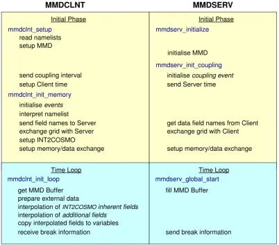
Fig. 5. Work flow of the MESSy submodels MMDCLNT and MMDSERV. The order of the subroutines corresponds to the calling sequence.
Subroutines in the same row exchange information/data with each other.
3. The server side of the MMD library receives and stores the names of the fields requested from the client model. 4. The server receives the geographical coordinates of the client model grid points. Based on those, the server de-termines the server grid segment required by the client for the interpolation. It has to cover the entire client domain plus an additional frame. The corresponding server grid information is sent back to the client. 5. The server determines an index list used by the MMD
library for the data exchange. To minimise the mes-sage passing traffic between the individual process enti-ties (PEs4), each server PE provides exactly those data points required by the respective individual client PE. The calculation of the index list associating the individ-ual grid points of the parallel decomposed server grid with the individual grid point in the in-coming coarse 4Here, PE is equivalent to an MPI task.
(also parallel decomposed) client grid5is explained in detail in the “MMD user manual” in the Supplement. 6. As last step of the initialisation, the server associates the
POINTERsto the fields requested for the data exchange. First, the server receives the names of the fields from the MMD library (see step 3 above). If required, the server further acquires the representation (i.e. the geometric layout) of the fields and sends it to the client. Finally, thePOINTERsare handed to the MMD library to access the requested data during the time integration phase. 7.2 Data exchange during the time integration phase
The MMDSERV submodel has to be called at the very be-ginning of the time loop to invoke the data exchange, i.e. it is called inmessy_global_start (see the right lower, cyan part of Fig. 5). MMDSERV tests individually for each 5This is the parallel decomposed grid on which the data of the
client, if the data exchange is desired within the current time step. In this case, new data is provided to the client by the MMD library subroutineMMD_S_FillBuffer. In this routine the MMD library uses the index list calculated dur-ing the initialisation phase (step 5 above) and thePOINTERs
to the data fields (step 6) to copy the required data into the memory buffer to be accessed by the respective client PE.
In addition, to synchronise the interrupt of all models of a model cascade, a server sends each time step the information to the client, whether the simulation is going to be interrupted after the current time step. Such an interruption, followed by a restart, is indispensable for longer simulations to fit the simulation into the time limitation dictated by the scheduling system.
8 The client submodel MMDCLNT
The MESSy submodel MMDCLNT manages the data acqui-sition, the data exchange with the server model, the succes-sive interpolation and the supply of the interpolated data to the client model. MMDCLNT distinguishes three different destination types of data fields provided to the client model:
a. initial fields, b. boundary fields and c. input fields.
The stand-alone INT2LM handles initial and boundary fields. Initial fields are only required for the very first step of the simulation and used to initialise the client variables (e.g. temperatureT, pressure deviationpp, water vapourqv, etc.). During the simulation the COSMO model is only sup-plied with boundary fields. They are copied to the bound-ary variables within the COSMO model (e.g.t_bd,pp_bd orqv_bd). MMDCLNT and INT2COSMO have been ex-panded to interpolate additional fields, i.e. fields that are not required by the stand-alone COSMO model, but by the MESSy submodels (e.g. tracers, emission flux fields etc.). The transfer and interpolation of additional fields up to rank 4 is possible (see Sect. 8.3.1). The stand-alone INT2LM processes only boundary fields for the COSMO model in-tegration phase. But, for COSMO/MESSy it is desired to exchange also fields required for the entire model domain (in comparison to those prescribed at the lateral domain bound-aries), e.g. emission flux fields, ozone climatologies etc. For the processing of these fields the third data destination type has been added, the so-called input fields. The input fields are interpolated in the same way as the initial and bound-ary fields and afterwards transferred to the respective target variables. This is performed in each coupling time step (see Sect. 8.3.2).
The number of fields to be provided by the server to the client and their destination type is flexible as the list of
exchanged fields is determined by the MMDCLNT namelists in the namelist filemmdclnt.nml(see Sect. 8.1).
8.1 The MMDCLNT namelist
The namelists of the submodel MMDCLNT are a vital part of the entire coupling procedure. For each coupled instance, it consists of two parts:
– The&CPL-namelist determines the time interval for the data exchange from the server to the client.
– The server dependent CPL-namelists &CPL_ECHAM and &CPL_COSMOcontain lists with the information about the fields, which need to be exchanged. These lists include the names of the channel objects in the memory management interface, information about the interpolation method and the destination of the field in the client model. Both namelists (&CPL_ECHAMand &CPL_COSMO) consist of two blocks: mandatory fields and optional fields. Mandatory are those fields, which are absolutely required for the COSMO basemodel6 and/or are needed for the interpolation procedure itself. The variables required by the COSMO model depend on the COSMO model setup, thus the list of mandatory fields varies between different setups. Optional fields are mostly additional fields, i.e. fields not taken into ac-count in INT2COSMO, but required by MESSy sub-models. For additional fields the interpolation methods must be specified in the namelist. The horizontal in-terpolation method can be either “Q” (quadratic), “L” (linear) or “M” (match interpolation). For further infor-mation about the interpolation methods we refer to the INT2LM documentation7. Additional namelist param-eters switch whether the field is interpolated also ver-tically, and whether monotonicity and/or positive defi-niteness are required for the interpolation result. Last but not least, the namelist entries determine the destination of the interpolated fields. We distinguish three destination types (see above): initial, boundary and/or input fields. Mandatory fields can be initial and boundary fields. For the optional fields the choice of initial and/or boundary and of input destination is ex-clusive, as input already implies initial and the provi-sion of boundary data is meaningless, since the field is overwritten each coupling time step.
6There are also optional fields for the COSMO basemodel. For
instance, as not all driving models provide the ice water content, this is not absolutely required as in-field for INT2LM. If the ice water is not available, INT2LM deduces the ice water content from the specific humidity and the temperature.
7http://www.cosmo-model.org/content/model/documentation/
Examples and a detailed description of the namelists con-tained in the namelist filemmdclnt.nmlare provided in the “MMD user manual” (see Supplement).
In addition to the coupling of standard 2-D and 3-D data fields, the coupling of 4-D data fields is implemented. They are treated exactly in the same way.
8.2 Initialisation phase
For MMDCLNT the initialisation phase is split into two sub-routines. This is required, as the server model determines the timing (i.e. the start and the stop date and time) of the client model8. Since each server defines the timing of its clients, the coarsest model determines the timing of all coupled mod-els. This coarsest model is hereafter called the master server. 8.2.1 mmdclnt setup
The timing information is already required at the begin-ning of the initialisation phase of the basemodel. Thus, this data exchange proceeds at the first entry point of MESSy in COSMO (i.e.messy_setup). Figure 5 (left) sketches the procedure.
– Read namelist: first, the two namelists &CPL and (dependent on the server model) &CPL_ECHAM or &CPL_COSMOare read (see Sect. 8.1).
– Setup MMD: second, MMDCLNT and the client side of the MMD library are set up by defining client specific variables, the MPI-communicators required for data ex-change and MMD internal initialisations. After initial-ising MMD, data can be exchanged between the server and the client.
– Setup date/time: third, the client and the server are syn-chronised. To achieve this, the client sends the time interval (in seconds) for the data exchange (from the server to the client) to the server. Next, the client re-ceives the date settings from the server9. Based on these dates, the COSMO model and TIMER submodel time variables are redefined. Additionally, the client re-ceives the time step length of the server. It is used to ensure the synchronised interrupt of the entire model cascade. Otherwise, one of the models would end up in a dead-lock during MPI communication. An inter-ruption (and restart) of the model cascade is desirable for simulations exceeding the available time limits as defined by the scheduler of a super-computer. Thus the client model defines an event, which is triggered each server time step to exchange the information, whether or not the server model will be interrupted after the cur-rent time step, the so-called break event.
8The term “timing” does not include the model time step length! 9For the definition of the dates we refer to the “TIMER user
manual”, which is part of the Supplement of J¨ockel et al. (2010).
8.2.2 mmdclnt init memory
Depending on the data destination (initial, boundary or in-put) of the coupling fields, memory needs to be allocated dur-ing the initialisation phase. Therefore, the second part of the initialisation is performed in mmdclnt_init_memory. Since the coupling procedure requires the presence of all other channel objects required for the coupling, mmdclnt_init_memory is called last within the en-try point messy_init_memory. The lower left part of the yellow box in Fig. 5 illustrates the work flow in mmdclnt_init_memory.
– Initialise events: at the beginning of mmdclnt_init_memory the coupling event and the break event are initialised, as now the TIMER is fully set up and the event manager is available. – Interpret namelist: because wildcards can be used
in the namelists for the client channel object names, these namelist entries have to be trans-lated into individual exchange fields in the subroutine interpret_namelist. Furthermore, the namelist entries are compared to the COSMO model variables yvarini and yvarbd, to ensure that the COSMO fields required by the basemodel setup are provided by MMDCLNT.
– Send field names to server: information from the namelist, required by MMD and the server, i.e. the channel and channel object names of each data field in the client and the server model (and their representa-tion), are stored in an MMD library internal list. Those parts of the list required by the server are sent to the MMD library part accessed by the server.
– Exchange grid with server: afterwards, information about the grids are exchanged between client and server. First, the client sends two 2-D-fields contain-ing the geographical longitudes and latitudes of the client grid. From this information and the definition of the server grid, the server calculates the required dimensions of the server grid section, which is trans-ferred to the client. INT2COSMO needs a segment of the coarse grid, which covers the complete COSMO model grid plus some additional space required for the interpolation to the finer grid.
The server sends back the complete definition of the in-coming grid, which, in the stand-alone INT2LM, is de-fined in the&GRID_INnamelist.
setup_int2lm dealing with the decomposition of the model domain and the parallel environment are skipped or replaced. Additionally, the routines reading the coarse grid data are omitted10.
– Setup memory/data exchange: the next step is the calcu-lation of an index list directly mapping each grid point of the parallel decomposed in-coming grid of the client to the respective grid point in the parallel decomposed domain of the server. The calculation is performed by the server. It requires the geographical coordinates of the client grid separately for each client PE as input (see also Sect. 7). The index list provides the basis for the efficient data transfer by the MMD library. It enables point-to-point data exchange from one server PE to one client PE, thus avoiding the gathering of the server fields and the scattering of the client in-fields before and af-ter the exchange, respectively. One of the most impor-tant features of this implementation of the coupling be-tween two models is its flexibility combined with the possibility to use the INT2LM interpolation routines as they are11. For all exchange fields listed in the namelist file of MMDCLNT, the data is processed automatically. For this a Fortran-95 structure was defined, contain-ing pointers to all fields (input, intermediate and target) used in MMDCLNT-INT2COSMO.
A detailed description of the memory allocation proce-dure is available in the “MMD user manual” (see Sup-plement).
In the last step of the initialisation phase, the POINT-ERsassociated to the in-fields are passed to the MMD library. Together with additional information about the dimensions of the fields and the index list determined before, within the MMD library the size of the exchange buffer is calculated and the buffer is allocated subse-quently.
8.3 The integration phase
The data exchange with the server takes place periodically within the time loop. As it provides the new input and/or boundary fields, this happens as early as possible within
10All modifications and extensions in the INT2LM and the
COSMO model code, which became necessary in the scope of the implementation of the on-line coupling are documented in the “MMD user manual” in the Supplement. The changes in the code are all enclosed in pre-processor directives.
11Thus, always the latest version of INT2LM can be used within
COSMO/MESSy. For instance, a newly introduced interpolation technique in INT2LM is directly available for the on-line coupling.
the time loop, i.e. in messy_init_loop12 for MMD-CLNT. In contrast to MMDCLNT, some fields need to be set in the server model before providing the data to the client. Thus for MMDSERV, the exchange is called at the end of messy_global_start. This is also important to avoid an MPI communication dead-lock: due to client and server dependenciesmmdclnt_init_loopmust al-ways be called beforemmdserv_global_startwithin the same basemodel.
First, MMDCLNT checks, if data exchange is requested in the current time step. If this is the case, the client acquires the data from the server by calling the MMD library subroutine MMD_C_GetBuffer. After this call, new data is assigned to all in-fields. Subsequently, the interpolation takes place (Sect. 8.3.1), after which the interpolated fields are copied (Sect. 8.3.2) to the target variables.
At the end of the subroutine mmdclnt_init_loop, when the current model time step coincides with a server time step, the information whether the simulation is inter-rupted after the current server time step is received. This information exchange is independent of the coupling inter-val and required to avoid an MPI communication dead-lock, caused by an interruption in the server model without inform-ing the client models beforehand.
8.3.1 Interpolation via INT2COSMO
The interpolation applied in MMDCLNT(-INT2COSMO) is based on the stand-alone program INT2LM as provided by the German Weather Service (DWD) for the interpolation of coarse grid model data to initial and boundary data re-quired by the COSMO model7. For the on-line coupling of the COSMO model to a coarse grid model (ECHAM5 or COSMO) as described here, it is necessary to perform the interpolation of the coarse grid data to the smaller scale COSMO model during the integration phase i.e. integrated into the basemodel itself. Therefore, INT2LM is imple-mented as submodel INT2COSMO into the MESSy sub-model MMDCLNT. The interpolation in MMDCLNT fol-lows the order of the stand-alone INT2LM program.
First, the external data are prepared13.
The subroutineexternal_datain INT2COSMO com-prises three sections:
12There is one exception: at the start of a simulation the data is
exchanged inmmdclnt init memory, because the initial fields are required already in the initialisation phase of a model simula-tion. The call inmessy init loopis therefore skipped in the very first time step (lstart=.TRUE.).
13The term external data refers to all data provided to the model
a. input of the external parameters needed by the COSMO model, external parameters are e.g. the orography, the leaf area index, the root depth or the land-sea fraction, b. import of the external parameters of the driving model,
and
c. definition of the internal setup and pre-calculation of variables required for the interpolation. Depending on the setup and on the fields provided by the driving model, missing fields are calculated from other avail-able fields.
The external parameters defined on the COSMO grid (item a) are usually constant in time. Thus they are read only during start or restart of a simulation. The import of the external pa-rameters of the driving model (item b) is replaced by the data exchange via MMD. Usually during the import, logicals are set indicating, which fields are provided by the driving model and which have to be calculated. As the import procedure is skipped in the on-line coupled setup, these switches are set within MMDCLNT according to the data sent via MMD in-stead. The last section (item c) is processed as in the stand-alone version.
The INT2LM inherent fields are interpolated first, calling the original interpolation routine org_coarse_interpol of INT2LM for the hori-zontal interpolation. The vertical interpolation of the INT2LM inherent fields is accomplished by the same subroutines as in the stand-alone version.
Afterwards, the additional fields are interpolated in the same way. First, each vertical layer (and each number di-mension) of a field is horizontally interpolated according to the interpolation type chosen in the namelist. This takes also into account the settings for monotonicity and positive defi-niteness (see Sect. 8.1). Second, the field is interpolated ver-tically, if requested.
8.3.2 Data transfer to COSMO variables
After finishing all interpolations the resulting intermediate fields are copied to the target fields. MMDCLNT distin-guishes three destination types for the data (see introduction to Sect. 8):
a. initial fields: These are only required for the initialisa-tion of the COSMO model,
b./c. boundary and input fields: These are updated periodi-cally during the model integration.
As fields of destination type (a) are only copied in the initial-isation phase, two independent subroutines perform the data transfer for data of type (a) and (b/c).
Moreover, there are two kinds of initial data:
a1. scalar variables defining the vertical model grid and the reference atmosphere of the COSMO model:
In the stand-alone INT2LM and COSMO model the vertical grid and the reference atmosphere are defined by namelist settings in INT2LM. The resulting vari-ables are dumped into the initial file and the COSMO model reads its grid and the reference atmosphere defi-nitions. In case of the on-line coupling, these variables are also defined by INT2COSMO namelist settings, but as COSMO does not read any file for input anymore, these variables also have to be transferred to the respec-tive COSMO variables14.
a2. 2-D-, 3-D- or 4-D-fields for the initialisation:
For these fields the contents of the intermediate field are copied to the target variable.
The subroutinemove_initial_arrays_to_COSMO copies both types of initial data to their counterparts of the COSMO/MESSy model.
During the integration phase two data destinations are dis-tinguished:
b. the boundary fields for prognostic variables; c. the input fields.
The most important difference between the on-line and the off-line coupling of the models is evident in the treatment of the boundary data. In the off-line setup boundary data are typically available for discrete time intervals (e.g. 6 hourly). The data at the beginning and the end of this time interval are read and the current boundary data in each time step are lin-early interpolated between these two. The on-line coupling works differently. To permit the same implementation as in the off-line mode, the server model would have to be one coupling time interval ahead. This would be possible for the 1-way-coupling. But the ultimate goal of our model devel-opments is the implementation of a 2-way-nesting. For this, the server model must not be ahead of the client model, oth-erwise the feedback to the larger scale model would not be possible. For simplicity, the two time layers of the boundary data are filled with the same value. As the on-line coupling allows for much higher coupling frequencies, no further in-terpolation in time is required.
9 Implementation details
This section conveys some important details about the tech-nical implementation itself.
9.1 Changes in the original codes of COSMO, INT2COSMO and ECHAM5/MESSy
All changes in the original COSMO and INT2LM code have been introduced with pre-processor directives. As different 14The variables in this category are vcflat, p0sl, t0sl, dt0lp,nfltvc,svc1,svc2,ivctype,irefatm,delta t
model configurations are possible, three pre-processor direc-tives have been introduced:
–
MESSY
–
I2CINC
–
MESSYMMD
The directive
MESSY
is used for the implementation of the MESSy interface into the COSMO model as described in Kerkweg and J¨ockel (2012). According to J¨ockel et al. (2005), all MESSy specific entry points in the COSMO model are encapsulated in#ifdef MESSY CALL messy_... #endif
directives. Those parts of the COSMO model, which become obsolete by using the MESSy interface are enclosed in
#ifndef MESSY ...
#endif
directives. Thus, it is always possible to use the original stand-alone COSMO model by simply not defining the pre-processor directive
MESSY
for the compilation.The directive
I2CINC
(INT2COSMO IN COSMO) is used for the modifications of the code required for the im-plementation of INT2COSMO as MESSy sub-submodel. As the COSMO model and INT2LM contain many redundant code parts, most changes in INT2COSMO exclude redun-dant code and variable definitions. The only changes in the COSMO code occur within the filesrc_input.f90, where the reading of the initial and boundary files is omitted. The directiveMESSYMMD
indicates that the MMD li-brary is used. In this case, more than one model instance runs concurrently within the same MPI environment. There-fore, the MPI-communicators used in each basemodel must be modified.MESSYMMD
andI2CINC
are two completely inde-pendent directives. In future the MMD library might be used to couple other models than ECHAM5 and COSMO. Thus, the directiveMESSYMMD
does not imply thatI2CINC
must also be defined. Vice versa, INT2COSMO in COSMO (and thusI2CINC) without defining
MESSYMMD
will be applicable in future to include the possibility to drive COSMO/MESSy off-line, directly with ECHAM5/MESSy or COSMO/MESSy output. Instead of receiving the data on-line from MMD, files containing the required data from the coarser model are imported and interpolated on-line by INT2COSMO.9.2 Implementation of INT2LM as MESSy sub-submodel MMDCLNT-INT2COSMO
For the on-line coupling method described here, the interpolation of the coarse grid data to the smaller scale COSMO model is performed during the time in-tegration. Therefore INT2LM is implemented as submodel MMDCLNT-INT2COSMO into the MESSy sub-model MMDCLNT. Consequently, INT2COSMO co-exists within the COSMO/MESSy model itself.
Many subroutines and tools are part of both, the INT2LM code as well as of the COSMO model code. Those subrou-tines available in both models are used from the COSMO code for both model parts. Technically, INT2LM was in-cluded into the MESSy code distribution as stand-alone basemodel INT2COSMO within the MESSy basemodel di-rectory (mbm). For the inclusion in COSMO/MESSy a directory parallel to the source code directory of COSMO (cosmo/src) calledcosmo/src_i2cwas cre-ated, which contains links to those source code files of the mbm model INT2COSMO, which are required in the MMD-CLNT submodel INT2COSMO.
To reduce the MPI communication overhead result-ing from the different parallel decompositions of the INT2COSMO and the COSMO model grid, the core regions of the COSMO and the INT2COSMO grid have to be con-gruent15. The “MMD user manual” (see Supplement) con-tains a detailed explanation of the procedure used to adjust the parallel decomposition of the INT2COSMO grids to the parallel decomposition of the COSMO model grids.
At the time being, the only server models available within the MESSy system are the ECHAM5/MESSy and the COSMO/MESSy model. Therefore, the module files of INT2LM, which are only relevant for other driving models, are unused in INT2COSMO so far, but can be easily activated if required.
More details about the implementation of INT2COSMO into MMDCLNT are provided in the “MMD user manual” in the Supplement.
10 Remarks on optimising the run-time performance efficiency
The main challenge in efficiently using the available com-puter resources, (the CPU time) with MECO(n), is to find the optimum distribution of MPI tasks among the participat-ing model instances. This optimum distribution depends on the chosen model setups, the model resolutions, the num-ber of instances etc. and usually underlies further constraints. 15This is not trivial, as the “inner” INT2COSMO grid is the
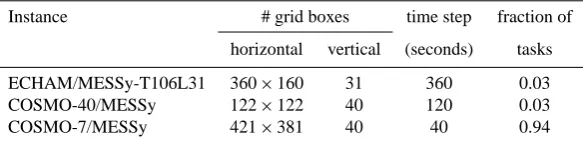
Table 1. Fraction of MPI tasks for the different MECO(2) instances estimated for a maximum efficiency from the number of grid boxes and
time step lengths.
Instance # grid boxes time step fraction of horizontal vertical (seconds) tasks ECHAM/MESSy-T106L31 360×160 31 360 0.03 COSMO-40/MESSy 122×122 40 120 0.03 COSMO-7/MESSy 421×381 40 40 0.94
Such constraints can be both, intrinsic to the models (e.g. if the number of usable tasks has a resolution dependent up-per limit caused by the chosen parallel decomposition), or posed by the used computer system (e.g. if only specific task numbers (e.g. full nodes) are selectable). As a consequence, a general statement on the optimum distribution of tasks is hardly possible.
To facilitate the optimisation process, both MMD sub-models measure on-line the waiting times between the cor-responding requests and the time they actually read (MMD-CLNT) and wrote (MMDSERV) the MMD exchange buffer. These times are provided as channel objects and therefore (optionally) subject to output. These times in combination with the on-line measurement of wall-clock and CPU-times of the submodel QTIMER (J¨ockel et al., 2010) provide valu-able information to assess the run-time performance effi-ciency.
With an example, we provide a general guideline. The chosen MECO(2) setup is the one used by Kerkweg and J¨ockel (2012) and Hofmann et al. (2012), i.e. two COSMO/MESSy instances nested into each other are nested into the global ECHAM/MESSy. The COSMO/MESSy do-mains are the bluish coloured dodo-mains over Europe in Fig. 1. To start with a first guess, we make the crude assumption that each grid box in each model instance at each time step requires the same computing time. To achieve an optimal load balance between the model instances, this defines the relative distribution (fraction) of tasks among the model in-stances, so far without further constraints. For the chosen example the numbers are listed in Table 1, meaning that, un-der the assumption above, load balance is achieved, if out of one hundred tasks, three are assigned to ECHAM/MESSy, three to the coarse COSMO-40/MESSy instance, and 94 to the finer COSMO-7/MESSy instance.
Next, we assess the constraints exposed by our com-puter system, the IBM Power6 system “blizzard” at the “Deutsches Klimarechenzentrum”, Hamburg (DKRZ, http: //www.dkrz.de/). This computer has 16 dual core proces-sors per node and we can only use complete nodes, i.e. multiples of 32 tasks16. According to Table 1, we assign 16For simplicity, we do not use the possible Simultaneous
Multi-threading (SMT) Mode with 64 tasks per node here and only assign one task per core.
ECHAM/MESSy and COSMO-40/MESSy 4 tasks each, and hereafter assess the run-time performance efficiency for four different setups, namely with 24, 56, 88 and 120 tasks for COSMO-7/MESSy (i.e. using in total between 1 and 4 nodes with 32 CPUs each). The resulting waiting times are dis-played in Fig. 6. A perfect load balance and synchronisation between the different model instances would result in zero waiting times. This, however, is virtually impossible to be achieved, since the required computing time per model time step varies depending on the model setup. For instance, radi-ation is not calculated every time step and output is only trig-gered at distinct time intervals (hourly in the example here).
As Fig. 6 shows, the COSMO-7/MESSy client is much too slow in the 4-4-24 setup, as both servers wait, while the clients do not. In the 4-4-56 setup the server waiting times are reduced by a factor of approximately 2 (implying a nearly linear scaling) and waiting times for the coarser client emerge. For the 4-4-88 setup, both clients experience idle times regularly exceeding the server waiting time, except at full hours, when the output is written. For the 4-4-120 setup the maximum waiting times of server and clients are similar. But, because the servers run with less tasks, the overall idle time in this last setup is longer as in the other setups. Figure 7 displays for the four setups the average waiting time per task calculated according to
¯ Tw= 1
3 P
i=1 ni
2 X
s=1
Tw,sns+
3 X
c=2 Tw,cnc
!
(1)
wherenis the number of tasks used for each model instance (indexi), distinguished for the servers (indexs) and for the clients (indexc), respectively andTware the individual wait-ing times. While the 4-4-24 (black line) setup produces rel-atively constant idle times of 3 seconds on average per task, the average waiting times in the setups with more tasks for the COSMO-7/MESSy client (4-4-88 and 4-4-120, green and blue lines, respectively) peak to 4 or 7 seconds, respectively, with smaller waiting times in between these peaks. The best balanced setup is the 4-4-56 setup (red line) as it produces the shortest average waiting times.
Fig. 6. Waiting times of the server and clients required for the four
task distributions 4-4-24, 4-4-56, 4-4-88 and 4-4-120. The black and the green lines denote the time the ECHAM/MESSy and the COSMO/MESSy server tasks wait, respectively. The red and the blue lines indicate the waiting times of the COSMO-40/MESSy and the COSMO-7/MESSy clients, respectively.
Fig. 7. Average waiting time per task (according to Eq. 1) for the
different setups (black: 24, red: 56, green: 88 and 4-4-120: blue).
as shown in Table 2. The table lists the average wall-clock times (in seconds) per simulated hour and the correspond-ing consumed CPU-time (in hours). As to be expected, as long as the communication overhead (including the waiting times) does not outperform the calculation effort, more tasks result in shorter wall-clock times. However, the speedup for the assessed MECO(2) cascade slows down considerably for the 4-4-120 setup, implying that no further speedup can be expected, if only the number of tasks for the COSMO-7/MESSy instance is further increased. As Table 2 further shows, the best efficiency is achieved with the 4-4-56 setup, because the costs in terms of used CPU-time per simulated hour show a minimum. This is the setup, for which we de-duced above that it accumulates the least idle times and is therefore best balanced.
As a result, our first guess based on the crude assumption, (see Table 1) is not the best (i.e. most efficient) choice, be-cause we need to take into account the accumulated wait-ing times. As this example shows, the optimum distribu-tion of tasks cannot be estimated straightforwardly. How-ever, the MMD submodels MMDCLNT and MMDSERV are equipped with internal watches to measure their waiting times for the data exchange between the model instances. In combination with the MESSy submodel QTIMER this pro-vides a convenient way for empirically determining the opti-mum choice with only a few short model simulations in the desired MECO(n) setup.
11 Summary and outlook
Table 2. Average wall-clock (seconds) and corresponding
times (hours) per simulated hour for the different setups. The CPU-times are the product of the wall-clock CPU-times and the number of used cores. In our setup the number of cores equals the number of MPI tasks.
Setup wall-clock CPU-time Setup (s) (h) 4-4-24 280.0 2.49 4-4-56 133.6 2.38 4-4-88 114.3 3.05 4-4-120 102.8 3.77
cascade as MECO(n) (MESSy-fied ECHAM and COSMO nested n times). Hence, the example in Fig. 1 shows a MECO(12) setup, i.e. 12 COSMO/MESSy instances nested into ECHAM5/MESSy. To further visualise the structure of the nested instances “n” (heren=12) can be written as the sum of the individual cascades. For the example shown in Fig. 1 one can write MECO(2+2(1+1)+2(1+2))as two single COSMO/MESSy (“2”), 2 COSMO/MESSy instances with one further nest (“2(1+1)”) and 2 COSMO/MESSy in-stances with 2 nests on the next nesting level (“2(1+2)”) are nested into ECHAM5/MESSy. Further examples of MECO(2) model setups are presented in the companion arti-cles (Kerkweg and J¨ockel, 2012; Hofmann et al., 2012).
While the regional atmospheric chemistry model COSMO/MESSy (Kerkweg and J¨ockel, 2012) was de-veloped to provide a limited-area model for atmospheric chemistry applications, the main goal for the development of MECO(n) is to provide consistent dynamical and chemical boundary conditions to a regional chemistry model in a numerically efficient way and thus providing a zooming capability. Chemical calculations demand a much higher number of exchanged fields (all tracers except the very short lived species need boundary conditions) and a higher frequency for the provision of the boundary data (necessary to capture the diurnal variations of chemical compounds). Therefore, an off-line coupling (as usually performed for the mere meteorological simulations) becomes impracti-cable due to the enormous amount of data and numerous pre-processing steps. Thus, we couple the models on-line in a client-server approach: the server model provides the input data via MPI based communication during the integration phase and the client model interpolates these data to get its boundary and input data. Hence, with this new approach
– no additional disk storage is required to keep the files containing the preprocessed initial and boundary data available during the regional model simulation,
– a higher frequency for boundary data provision becomes possible.
– the data exchange is faster, because data exchange via memory is much faster compared to disk input/output, – no stand-alone interpolation program needs to be run
for each time step, for which boundary data is provided to the regional model, i.e. no more pre-processing steps are required, that could only be performed sequentially, whereas in our approach the models run concurrently, – the input and boundary data files, as used by the
stand-alone COSMO model for the meteorological variables, are no more needed in the on-line coupled setup. This leads to a further reduction of the required disk storage, – a prerequisite for two-way nesting, i.e. feedback from
the smaller to the larger scales is fulfilled.
Thus, much less disk storage is required for an on-line cou-pled simulation and manual data processing to produce the boundary files is largely reduced.
On the other hand, the on-line coupled setup requires more computing power at once compared to the stand-alone setup, as all models run concurrently in the same MPI environment. Nevertheless, nowadays at super-computing centres, it is eas-ier to access a large number of computing cores, than large amounts of permanently available disk storage.
The on-line data exchange is managed by the newly de-veloped Multi-Model-Driver (MMD) library and two corre-sponding MESSy submodels, MMDCLNT and MMDSERV. During the initialisation phase the models communicate via MMD usingMPI_sendorMPI_recvand the group com-municators defined for one client-server pair. During the integration phase, the exchange of the data fields required by the client is coded as point-to-point, single-sided, non-blocking MPI communication: the server fills a buffer and continues its integration, while the client reads the data stored by the server.
The MMD library could be used to couple other mod-els as well, but the interfaces to the ECHAM/MESSy and the COSMO/MESSy models (i.e. the submodels MMD-SERV and MMDCLNT) are rather specific for MECO(n) and need to be adapted; in particular, as MMDCLNT includes INT2COSMO, which is tailor made for grid-transformations to the COSMO model grid. Nevertheless, the adaption is straightforward due to the standardised MESSy infrastruc-ture.
The partitioning of the available MPI tasks between the model instances for an efficient usage of resources is left to the user, since its optimum strongly depends on the individ-ual model setups. To facilitate this task, the MMD submodels are equipped with internal stopwatches to measure the per-formance. With this information, the optimisation procedure as shown, requires only a few short simulations with different task distributions.
Finally, we emphasise that even though the technical struc-ture looks complicated at the first glance, the user only needs to edit the run-script and the MMDCLNT namelist files (one per client instance) to run MECO(n).
Appendix A
Classification of different coupling approaches
In the Earth system modelling community the terms cou-pling, coupler and coupled are widely used to describe a vari-ety of aspects of connections within an Earth System Model (ESM), though rarely precised. In general, these terms are used to express some way of how different components in-fluence each other. For instance the basic equations describ-ing the system form a set of coupled differential equations, however, these equations are commonly not regarded as com-ponents of the model.
This intrinsic level of coupling is complemented by a sec-ond level of coupling, which arises from the (numerical) ne-cessity to formulate and implement complex ESMs in an op-erator splitting approach: the different opop-erators need to be coupled together to form an integral model: one operator after each other modifies the state variables of the system. Technically, the simplest operator is formed by a subroutine, which calculates a specific output for the provided input. The granularity of this decomposition into operators can be for-malised in a way that a set of subroutines describes a specific natural process of the system (which in MESSy is called a submodel, J¨ockel et al., 2005). Such a process can still be regarded as an operator. Even further, a set of processes de-scribing a specific domain of the Earth system, such as the atmosphere or the ocean subsystem, can still be regarded as an operator.
The coupling then describes, how these operators commu-nicate which each other. Two operators are internally cou-pled, if they are part of the same program unit, i.e. the same executable, and exchange information on-line, i.e. via the working memory. In contrast to that, operators are exter-nally coupled, if they are split into different program units, i.e. different executables. This implies that information to be exchanged between the operators necessarily need to leave the program unit bounds and are either exchanged off-line via storage and import to/from an external (e.g. disk-based) file system, or on-line via the working memory. Whereas off-line external coupling is computationally inefficient due to the low input/output bandwidths and hardly allows a two-way data exchange, on-line external coupling requires spe-cial software and/or a model infrastructure for the commu-nication between two (or more) executables (such as for in-stance the message passing interface, MPI).
The external on-line coupling approach can be further differentiated into the indirect external on-line coupling, in which two different program units communicate via an
additional intermediate program unit (meaning that another executable is required, which is not identical to the mes-sage passing environment process) and into the direct ternal on-line coupling, where the two program units ex-change their information without such an additional interme-diate program unit (e.g. within the same message passing en-vironment). The intermediate program unit performing the data exchange in the indirect external on-line coupling ap-proach is commonly called a coupler and, in most implemen-tations, does not only perform the data exchange (including transpositions) but contains further services, such as for in-stance rediscretisations, i.e. transformations of data from one model grid to another.
Appendix B
Glossary
– additional field: an additional field is a field requested in the MMDCLNT namelist in addition to the fields al-ready taken into account within INT2COSMO.
– boundary field: it is used to prescribe the variables at the model domain boundaries.
– break event: the break event is an event that is triggered each server time step in order to receive the information from the server, whether the server model is going to be interrupted after the current time step or not.
– channel: the generic submodel CHANNEL manages the memory and meta-data and provides a data transfer and export interface (J¨ockel et al., 2010). A channel rep-resents sets of “related” channel objects with additional meta information. The “relation” can be, for instance, the simple fact that the channel objects are defined by the same submodel.
– channel object: it represents a data field including its meta information and its underlying geometric struc-ture (representation), e.g. the 3-dimensional vorticity in spectral representation, the ozone mixing ratio in Eule-rian representation, the pressure altitude of trajectories in Lagrangian representation.
– coupling event: this is an event scheduling the data ex-change from the server to the client. Its time interval has to be a common multiple of the client and the server time step length.