www.geosci-model-dev.net/5/223/2012/ doi:10.5194/gmd-5-223-2012
© Author(s) 2012. CC Attribution 3.0 License.
Geoscientific
Model Development
Wavelet-based spatial comparison technique for analysing and
evaluating two-dimensional geophysical model fields
S. Saux Picart, M. Butensch¨on, and J. D. Shutler
Plymouth Marine Laboratory, Prospect Place, The Hoe, PL1 3DH Plymouth, UK Correspondence to: S. Saux Picart ([email protected])
Received: 26 October 2011 – Published in Geosci. Model Dev. Discuss.: 24 November 2011 Revised: 2 February 2012 – Accepted: 8 February 2012 – Published: 13 February 2012
Abstract. Complex numerical models of the Earth’s
environ-ment, based around 3-D or 4-D time and space domains are routinely used for applications including climate predictions, weather forecasts, fishery management and environmental impact assessments. Quantitatively assessing the ability of these models to accurately reproduce geographical patterns at a range of spatial and temporal scales has always been a difficult problem to address. However, this is crucial if we are to rely on these models for decision making. Satel-lite data are potentially the only observational dataset able to cover the large spatial domains analysed by many types of geophysical models. Consequently optical wavelength satel-lite data is beginning to be used to evaluate model hindcast fields of terrestrial and marine environments. However, these satellite data invariably contain regions of occluded or miss-ing data due to clouds, further complicatmiss-ing or impactmiss-ing on any comparisons with the model. This work builds on a published methodology, that evaluates precipitation fore-cast using radar observations based on predefined absolute thresholds. It allows model skill to be evaluated at a range of spatial scales and rain intensities. Here we extend the original method to allow its generic application to a range of continuous and discontinuous geophysical data fields, and therefore allowing its use with optical satellite data. This is achieved through two major improvements to the origi-nal method: (i) all thresholds are determined based on the statistical distribution of the input data, so no a priori knowl-edge about the model fields being analysed is required and (ii) occluded data can be analysed without impacting on the metric results. The method can be used to assess a model’s ability to simulate geographical patterns over a range of spa-tial scales. We illustrate how the method provides a compact and concise way of visualising the degree of agreement be-tween spatial features in two datasets. The application of the new method, its handling of bias and occlusion and the ad-vantages of the novel method are demonstrated through the analysis of model fields from a marine ecosystem model.
1 Introduction
with specific space and time scales, which may vary consid-erably between applications and will depend upon the data that is being analysed. To fully assess these models the identification of the model skill over a range of spatial and temporal scales is crucial. Additionally, allowing the dis-tribution of the data being analysed to guide the setting of any aggregation levels would allow approaches to be more generic. Relatively recent work in the field of precipitation forecast analysis has seen the development of techniques for studying two-dimensional binary difference maps using Haar wavelets (Casati et al., 2004; Casati, 2010). This work is it-self based on an earlier study from Briggs and Levine (1997) who used wavelet decomposition in field forecast verifica-tion. The binary maps, defined for specific thresholds of the geophysical dataset, are the result of differencing the two in-put datasets, while the use of the Haar wavelet allows the identification of the orthogonal spatial structures responsible for any differences. Haar wavelets (Haar, 1910) are discon-tinuous and are therefore suitable for handling spatially dis-continuous data fields. The approach of Casati et al. (2004) was recently applied to analysing the performance of a hy-drodynamic ecosystem model (Shutler et al., 2011). In both situations, the thresholds of the different parameters used to generate the binary difference maps were manually set, based on user experience, and therefore the evaluation results are likely to vary with respect to the thresholds chosen.
Satellite or Earth observation data provide an excellent dataset to evaluate model fields. Indeed, Earth observation is one of the few sources of data that can provide the required spatially-continuous datasets needed to evaluate the outputs of large spatial coverage geophysical models. Visible and in-frared remote sensing data can be used to evaluate global ma-rine hydrodynamic ecosystems models (Shutler et al., 2011) through two major variables: chlorophyll-a surface concen-tration and sea surface temperature. However, visible tral wavelengths between 400–600 nm) and infrared (spec-tral wavelengths between 700–1000 nm) fields of the oceans measured from a satellite will invariably contain occluded or missing data due to clouds (e.g. the optical sensor is unable to see through cloud). This can present a problem when using these data to evaluate model fields as (in contrast) the model fields will be spatially complete. Removing the equivalent data from the model data before comparison with the Earth observation data (e.g. as done by Shutler et al., 2011) is a simple way of addressing that issue. However, dependent upon the dataset, this can have a significant impact upon the statistical distribution of the dataset being analysed, and thus can potentially impact on any evaluation results.
In this paper, the original method of Casati et al. (2004) has been extended to handle regions of missing or occluded data, while maintaining the orthogonality of the wavelet ap-proach. Furthermore, to make the methodology more objec-tive and to enable the generic application of the approach to alternative applications (e.g. other geophysical models), the thresholds are determined based on the statistical distribution
of each input dataset. This produces a comparison of the spatial structures inherent to each dataset (as shall be illus-trated below) comparing extremes of one set to extremes of the other and average conditions to average conditions. To illustrate its application this new approach has been applied to assess the performance of important state variables of a dynamic marine ecosystem model, comparing the output to data derived from satellite Earth observation. The technique is equally applicable to alternative scenarios including eval-uating the performance of precipitation and climate forecast models. The paper is structured as follows. Section 2 gives a description of the methodology developed as well as an overview of the original methodology of Casati et al. (2004), highlighting the novel enhancements. Section 3 illustrates its application, followed by a discussion about the benefits of-fered. Section 4 gives a summary of the methodology along with possible applications.
2 Methodology
The methodology we propose here evaluates the match of two-dimensional representations of two datasets at distinct spatial scales through wavelet decomposition. This section gives a brief overview of the original methodology of Casati et al. (2004) and a detailed description of the novel exten-sions.
2.1 Overview of original method
The original methodology was developed by Casati et al. (2004) for verifying spatial precipitation forecasts. It con-sists of a suite of simple operations carried out on a set of user-defined thresholds of the variable of interest. A met-ric comparing spatial maps based on these thresholds (or cutoffs) then summarises the ability of a model to simulate the geophysical structures under investigation. The different steps of this process for a particular threshold are described briefly:
– Computing the binary fields for the two datasets,
respec-tively: for a given thresholdtand a data field D, the bi-nary image I is defined by: I=1 where D≥tand I=0 where D< t.
– Computing the binary difference map: subtraction of
the corresponding binary fields.
– Performing a 2-D-Haar wavelet decomposition on the
binary difference map.
– Computing the mean square error and skill score for
2.2 Enhanced method
The method outlined above allowed the authors to evaluate the forecast skill as a function of precipitation rate and spa-tial scale. Shutler et al. (2011) applied the method for evalu-ating the performance of a hydrodynamic-ecosystem model. However, occluded data was handled very simply resulting in a loss of orthogonality hence skills at scales subject to oc-clusion were affected by smaller scale errors. Additionally, the thresholds used to generate the binary maps were set at arbitrary absolute levels.
A modified version of this wavelet analysis is hereafter presented in generic terms.
2.2.1 Binary difference maps
The whole methodology is based on the concept of binary difference maps. The degradation of the continuous field to a binary map is a crucial step as it defines the patterns in the datasets that are going to be compared. Instead of using absolute thresholds to define the binary difference image (as was used in the original methodology by Casati et al., 2004), we apply the methodology over ranges inherent to the data sets as suggested by Yates et al. (2006). These ranges are defined by the quantiles of the data distribution, evaluated for each of the two datasets independently. For example, if we consider the variableV, we may define quantilesV0 %=
Vmin;V20 %;V40 %;V60 %;V80 %andV100 %=Vmax. These
quantiles can then be used to define five intervals in each of the datasets: [V0 %,V20 %),[V20 %,V40 %); [V40 %,V60 %);
[V60 %,V80 %);[V80 %,V100 %]. The methodology allows for
any number of quantiles. However, here for simplicity we have chosen to use the five ranges defined above.
Considering two 2-D spatial fields X and Y, and follow-ing the notation of Shutler et al. (2011) we define the binary masks for the two data fields (IY) and (IX) by:
IX=
1, Xq1≤X< Xq2
0, else
IY=
1, Yq1≤Y< Yq2
0, else,
(1)
whereXq1, Xq2 (Yq1, Yq2 respectively) are two
consecu-tive quantiles for each dataset, defining what we will refer to, in the following, as q, quantile range ([Xq1,Xq2) and
[Yq1,Yq2), respectively). We note here that if we chose
equally-spaced quantiles the number of data points attributed to each range would be identical for both data fields. This is an important improvement with respect to the original methodology because it allows the study of inherent patterns in the two images, removing the need for absolute thresholds values.
From these two binary masks we then compute the bi-nary difference map Z, defined by Z=IY−IX, and noted Zqwhen referring to the quantile rangeq.
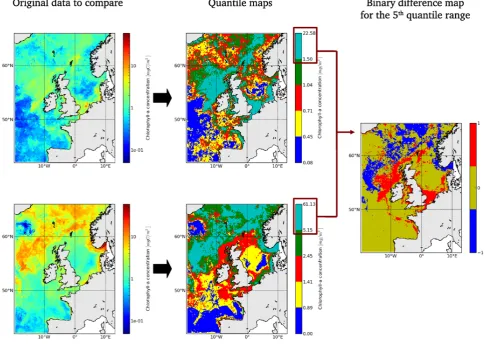
Figure 1 illustrates the process of creating a binary differ-ence map for ocean chlorophyll-a data obtained from model and satellite imagery. In the left column of Fig. 1 are the satellite estimates (top), and the model estimates (bottom). From these two fields, quantile maps are derived (second col-umn on the same figure), that show the patterns associated with the quantile definition. By subtracting these two maps we obtain the binary difference map (right-hand side map on Fig. 1) which is fed into the wavelet decomposition described in the next section (Sect. 2.2.2).
2.2.2 Wavelet decomposition
The binary difference map as defined above is decomposed using an improved wavelet decomposition technique with re-spect the original one presented by Casati et al. (2004). We introduce into the wavelet decomposition a weight imageζ0
that reduces the impact of heavily occluded areas on the dif-ference metrics while preserving the orthogonality between the scale components:
ζ0=
1 for valid data
0 for missing data (2)
As described by Casati et al. (2004), a two-dimensional dis-crete Haar wavelet decomposition can be performed by spa-tially averaging over a 2l×2l pixel region, where l is the level of decomposition. We define the l-th father (Wlfather) and mother (Wlmother) wavelet component by:
Wlfather(Zq)=
hZqζ0i2l×2l
hζ0i2l×2l
(3)
Wlmother(Zq)=Wlfather−1 (Zq)−Wlfather(Zq) (4)
where the notationh·i2l×2l refers to a 2l×2l spatial averag-ing. Thel-th father wavelet component is obtained by spa-tial averaging over 2l×2lpixels and is therefore a smoothed
representation of the original binary difference map. Thel-th mother wavelet quantifies the differences between the origi-nal binary difference map and the average generated by the father wavelet.
This decomposition is done retaining the original resolu-tion of the image, thus allowing to use the same weight im-age for each aggregation level. This formulation maintains the orthogonality and conserves the original signal contained in the split components, i.e.
Zq=WLfather(Zq)+
L
X
l=1
Wlmother(Zq) (5)
Fig. 1. Binary difference map creation. On the left: re-gridded satellite (top) and model (bottom) monthly fields of surface concentration of chlorophyll-a for May 2004. In the centre: quantile maps of the same fields (top, satellite; bottom model). On the right: binary difference map for the uppermost quantile range.
2.2.3 Mean squared differences and skill score
For each level of decomposition (l) and each quantile (q), the mean squared difference of the mother wavelet (MSEl,q) is
computed by: MSEl,q=
P
(Wlmother(Zq)ζ0)2
P ζ0
(6) whereP means summation over the whole domain. The inclusion ofζ0 allows any missing or occluded data to be
accounted for.
The overall mean squared difference is maintained through the decomposition and the following equation remains true:
MSEq= L
X
l=1
MSEl,q (7)
where MSEqrefers to the overall mean squared difference of
the binary difference map.
We then compute the skill score (SS) as defined in Casati et al. (2004) which is more intuitive to interpret than the MSE: 1 means a perfect match, 0 corresponds to the com-parison of random data, below 0 represents a match worse than due to random chance alone. The formulation of the skill score is as follow:
SSl,q=1−
MSEl,qL
2εq(1−εq)
(8) whereεq is the fraction of data contained in the quantileq.
The skill score is in fact defined as the mean square error relative to the means square error of a random no skill simu-lation (see Casati et al., 2004).
3 Results and discussion
3.1 Satellite data and hydrodynamic-ecosystem model
To accommodate the reader we give brief introductions to the data sets used in the examples. We shall not go into the details of the geophysical application and the implications of the skill assessment, but rather provide a quick overview to enable the reader to fully understand the methodology and its benefits. The data shown serve simply as examples to provide a show case for the methodology.
The model used in this work is an implementation of the POLCOMS-ERSEM model (Allen et al., 2001, 2007) for the dynamics of the lower trophic level of the marine ecosys-tem. It provides full four-dimensional data for hydrody-namic, organic and inorganic states of the marine ecosystem at a horizontal resolution of roughly 12 km and at tempo-ral scales of 15 min. In particular it provides fields for aver-age chlorophyll-a concentration and sea-surface temperature, which were used in this study.
To evaluate these model data, two satellite datasets were used:
– Globcolour chlorophyll-a global dataset. This dataset
consists of daily chlorophyll-a estimates at a spatial resolution of∼4 km (based on data from three optical wavelength satellite sensors).
– Pathfinder sea surface temperature (SST) global dataset.
This dataset consists of daily sea surface temperature estimates at a spatial resolution of∼4 km (based on data from a thermal infrared satellite sensor).
For a fair comparison, the region of interest (which is the model domain) is first extracted from the satellite global dataset. The extracted satellite data are then re-gridded to the coarser model grid using a bilinear interpolation.
As suggested by Shutler et al. (2011) we compute the op-tical depth averaged chlorophyll-a concentration to compare with satellite estimates of chlorophyll-a which are represen-tative of a variable depth depending on the constituent in the water. The model outputs are then cloud-masked on a daily basis using the contemporaneous satellite masks. Finally, monthly composites are created by averaging daily model and satellite data.
We then analyse all data for 2003–2004. The analysis pre-sented hereafter is based on the definition of five quantile ranges as described in Sect. 2.2.1. Each quantile range there-fore holds 20 % of the distribution and in Eq. (8) we always haveεq=0.2.
3.2 Spatio/temporal evaluation of the North East European shelf sea modelling
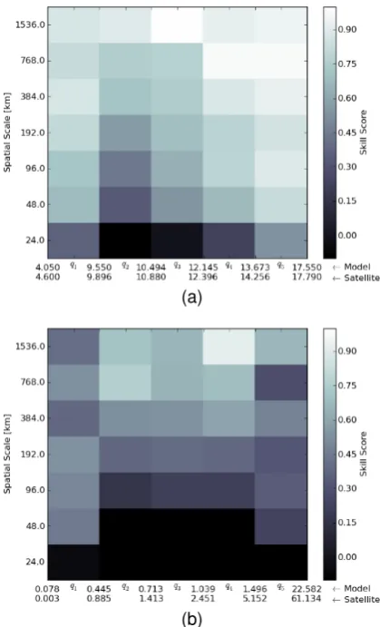
Figure 2 shows an example application of the methodol-ogy for fields of sea surface temperature (Fig. 2a) and chlorophyll-a concentration (Fig. 2b). Quantiles are reported on the x-axis with the corresponding lower and upper values
Discussion
P
ap
er
|
Discussion
P
ap
er
|
Discussion
P
ap
er
|
Di
scuss
ion
P
ap
er
|
(a)
(b)
Fig. 2
:
Spatial scales versus quantile ranges
plots for May 2004. Sea surface
temper-ature (a) and chlorophyll-a
concentration (b) skill scores.
20
Fig. 2. Spatial scales versus quantile ranges plots for May 2004. Sea surface temperature (a) and chlorophyll-a concentration (b) skill scores.
for the satellite and model data. The y-axis shows the spatial scale in kilometres (km).
The methodology highlights scales and ranges of skill. One can notice a lower skill score at small scales (24 km) for both SST and chlorophyll-a for almost all ranges. One can also note higher model skills for the lowest and the highest quantiles at all spatial scales for SST.
This is less true for chlorophyll-a, where a low model skill is observed at high spatial scale (of about∼700 km) for the last quantile (high value of chlorophyll-a). This can be con-firmed by looking at the corresponding binary difference map (right-hand map on Fig. 1) where large scale differences are clearly visible in the north of the domain. An interpretation for that observation is a spatial mismatch (or misplacement) of a large summer bloom of chlorophyll-a in the north of the domain.
P
ap
er
|
Discussion
P
ap
er
|
Discussion
P
ap
er
|
Di
scuss
ion
P
ap
er
|
(a)
(b)
Fig. 3
:
Spatial scales versus time
plot for the
5
thquantile (80-100%) 2003-2004. Sea
surface temperature (a) and chlorophyll-
a
concentration (b) skill scores.
21
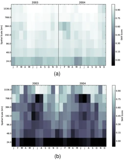
Fig. 3. Spatial scales versus time plot for the 5th quantile (80–
100 %) 2003–2004. Sea surface temperature (a) and chlorophyll-a concentration (b) skill scores.
Figure 3 shows a time/space skill score plot. Time has been reported on the x axis and spatial scale on they axis, the shades of grey represent the skill score of the wavelet decom-position for the 5th quantile. The 5th quantile corresponds to the upper range of sea surface temperature and chlorophyll-a, which in our example can be interpreted as extreme events (i.e. an algal bloom or a temperature anomaly).
Figure 3a shows that sea surface temperature skill score has high values throughout the year at all spatial scales for the 5th quantile. A small region of slightly lower skill score can be observed during January–March at spatial scales of about 200–400 km. We can also note a slightly lower skill score at low spatial scale throughout the year.
The chlorophyll-a skill score (shown on Fig. 3b) is gener-ally lower than the one of temperature and shows some inter-esting features. As for the sea surface temperature, we can observe a poorer skill score at low scale (first level of aggre-gation) throughout the year. However we can additionally observe a consistent patch of low skill in June–August be-tween 100 and 800 km. This pattern does not appear on the temperature skill score.
3.3 Interpretation of the skill score in terms of model evaluation
Low skill scores observed at small spatial scales (∼24 km) in both chlorophyll-a and SST model output can be explained by the high small scale variability in the satellite data that is not reproduced by the model. It is indeed easier to cap-ture low frequency variations and trends. Ocean colour and infrared remote sensing are strongly impacted by various sources of uncertainties including measurement noise, cali-bration noise or atmospheric correction uncertainties. How-ever, these results also illustrate the complexity of modelling biological systems.
The generally higher skill scores obtained for SST, at all scales and for all quantile ranges, (compared with chlorophyll-a) highlight the strength of the hydrodynamic model fed with high quality surface forcing and boundary conditions (Siddorn et al., 2007). One should also note that chlorophyll-a estimates from ocean colour data are represen-tative of a variable and unknown depth: the water leaving ra-diances (used to derive chlorophyll-a concentration) include contributions from the surface to a finite depth which varies with the optical properties of the water. For that reason, we choose to average the model chlorophyll-a over the optical depth (of the model), but an uncertainty still remains.
Finally, the consistent appearance of low skill scores in chlorophyll-a (5th quantile) analysis during June–August at large scale is correlated with the summer algal bloom off Scotland and Ireland coast. On the satellite chlorophyll-a field provided on the top-left map of Fig. 1, one can see high chlorophyll-a values (2–8 mg m−3) along the northwest coast
of Scotland and Ireland, whereas in the model field, the high-est chlorophyll-a values are observed further in the northwhigh-est direction and extend further toward the northwest coast of Norway. This translates into the large scale misplacement of pattern visible on the binary difference map (right map on Fig. 1).
3.4 Discussion
When comparing model output to another dataset, one may observe differences in the characteristics and possibly in the shape of data distributions. However, the model can still show some skill in representing relative patterns such as ex-treme events for example. It is therefore important to use a methodology which will be able to highlight the skill of the model without being affected by the bias or the data distribu-tion shape. The bias can be studied separately using simple classical methods but it is worth noting that one can compare the size and mean value of quantile ranges to study it in more detail (for each quantile range separately).
S. Saux Picart et al.: Wavelet-based spatial comparison technique for analysing and evaluating model fields 229
P
ap
er
|
Discussion
P
ap
er
|
Discussion
P
ap
er
|
Di
scuss
ion
P
ap
er
|
Fig. 4
: Illustration of the effect of a bias on the binary masks as defined in section
2.2.1.
a
and
b
are two sample data array where
b
displays a bias with respect to
a
.
c
and
d
are the binary masks obtained considering an absolute threshold that is the
overall mean value of
a
and
b
.
e
and
f
are the binary masks obtained using the quantile
approach introduced in section 2.2.1.
22
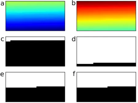
Fig. 4. Illustration of the effect of a bias on the binary masks as defined in Sect. 2.2.1. (a) and (b) are two sample data array where (b) displays a bias with respect to (a). (c) and (d) are the binary masks obtained considering an absolute threshold that is the overall mean value of (a) and (b). (e) and (f) are the binary masks obtained using the quantile approach introduced in Sect. 2.2.1.
version when using absolute thresholds. This is illustrated by Figs. 4 and 5. Starting from two 2-D data arrays that have exactly the same patterns but a systematic difference (bias), Fig. 4c and d illustrates how using absolute thresholds leads to completely different binary masks. However, using rela-tive thresholds (quantiles) enables the comparison of inherent spatial structures of the data sets (Fig. 4e and f).
Moreover, if we consider two data sets with the same pat-terns but different distributions (Fig. 5a–d), the binary masks defined by absolute thresholds are very different (Fig. 5e and f) and do not represent comparable structures. The use of quantile definitions provides a more robust definition of the patterns (Fig. 5e and f).
From the two illustrative examples described above, it is clear that if one would use absolute thresholds as break-off criteria for the binary maps, qualitatively similar patterns may appear to be structurally different. An additional benefit of the quantile definition is that it yields the same amount of data points in each quantile range hence guarantees equiva-lent structural maps.
The wavelet decomposition we described in Sect. 2.2.2 also provides more confidence to the results especially at the higher aggregation levels when comparing data sets with gaps. Applying the original method of Casati et al. (2004) to masked data, a cell (at high aggregation level) that con-tains very few valid values and a cell containing only valid values would have had the same impact on the overall MSE. The introduction of the weight imageζ0is a mathematical
solution that gives appropriate impact factors to each cell in relation to the data gap contained within it, while preserv-ing the fundamental characteristics of the decomposition, i.e. the orthogonality between the wavelet components and the conservation of the original signal (Eq. 5).
Discussion
P
ap
er
|
Discussion
P
ap
er
|
Discussion
P
ap
er
|
Di
scuss
ion
P
ap
er
|
Fig. 5
: Illustration of the effect of differences in distributions in the two datasets.
a
and
b
are two sample data arrays where
b
is a power function of
a
.
c
and
d
are their
respective histograms.
e
and
f
are the binary masks obtained considering an absolute
threshold that is the overall mean value of
a
and
b
.
g
and
h
are the binary masks
obtained using the quantile approach introduced in section 2.2.1, i.e. the median in
this case
23
Fig. 5. Illustration of the effect of differences in distributions in the two datasets. (a) and (b) are two sample data arrays where (b) is a power function of (a). (c) and (d) are their respective histograms. (e) and (f) are the binary masks obtained considering an absolute threshold that is the overall mean value of (a) and (b). (g) and (h) are the binary masks obtained using the quantile approach intro-duced in Sect. 2.2.1, i.e. the median in this case.
This methodology is based on statistically robust metrics and the choice of the threshold is driven by the data distribu-tion, and hence is more objective (for example this allows the study of patterns of extreme events of chlorophyll-a) in com-paring the inherent structures of the datasets. This is partic-ularly useful for temporal intercomparisons ie for situations where the bias in different time series is potentially different.
4 Conclusions
The results can be visualised in two very synthetic ways: a spatial scales versus quantile ranges plot, which can be used to identify the overall match/mismatch of the features in two 2-D data fields; and a spatial scales versus time plot, which can be used to analyse extreme events. Alternatively, if one is interested in a specific spatial scale, a time/quantile plot would provide useful information over the whole data range. This methodology, used in combination with other classi-cal ways of comparing two datasets, is a powerful evaluation tool (when comparing Earth observation data and model out-put) because it is objective and independent of the dataset distribution. It is therefore a very useful tool that can serve to justify or guide the choice of a model for a specific ap-plication. In the context of marine hydrological/ecosystem modelling these can be carbon budget, harmful algal bloom detection, ecosystem management.
One can also use this methodology as a way of comparing outputs from two different model. The method provides a synthetic way of representing the spatial effect of two differ-ent parametrisations, or the effect of using differdiffer-ent boundary conditions or forcing data in terms of spatial features.
Future work will concentrate on extending the approach to include the time dimension. This would enable a complete picture of the model skill to be considered including sea-sonal forecasts and the study of inter-annual or multi-decadal trends.
Supplementary material related to this article is available online at:
http://www.geosci-model-dev.net/5/223/2012/ gmd-5-223-2012-supplement.zip.
Acknowledgements. The authors would like to thank MyOcean
project for supplying Globcolour data for this study. The
AVHRR Oceans Pathfinder SST data were obtained from the
Physical Oceanography Distributed Active Archive Center
(PO.DAAC) at the NASA Jet Propulsion Laboratory, Pasadena, CA. http://podaac.jpl.nasa.gov. The authors thank the NERC Earth Observation Data Acquisition and Analysis Service (NEODAAS) for providing computing facilities and data storage. This work was funded by the UK NERC Oceans 2025 program theme 9, Next Generation Ecosystem Models. This work was partially supported by the EC FP7 MyOcean research and development project
“Improving CO2 Flux Estimations from the MyOcean Atlantic
north west shelf hydrodynamic ecosystem model (IFEMA)”. Edited by: J. Annan
References
Allen, J. I., Blackford, J. C., Holt, J. T., Proctor, R., Ashworth, M., and Siddorn, J. R.: A highly spatially resolved ecosystem model for the North West European Continental Shelf, Sarsia, 86, 423– 440, 2001.
Allen, J. I., Somerfield, P., and Gilbert, F.: Quantifying uncertainty in high-resolution coupled hydrodynamic-ecosystem models, J. Marine Syst., 64, 3–14, doi:10.1016/j.jmarsys.2006.02.010, 2007.
Bougeault, P.: The WGNE survey of verification methods for numerical prediction of weather elements and severe weather events, Tech. rep., Technical report, WMO, 2003.
Briggs, W. M. and Levine, R. A.: Wavelets and field forecast verifi-cation, B. Am. Meteor. Soc., 125, 1329–1341, 1997.
Casati, B.: New Developments of the Intensity-Scale
Tech-nique within the Spatial Verification Methods
Inter-comparison Project, Weather Forecast., 25, 113–143,
doi:10.1175/2009WAF2222257.1, 2010.
Casati, B., Ross, G., and Stephenson, D.: A new intensity-scale ap-proach for the verification of spatial precipitation forecasts, Me-teorol. Appl., 11, 141–154, 2004.
Doney, S. C., Lima, I., Moore, J. K., Lindsay, K., Behrenfeld, M. J., Westberry, T. K., Mahowald, N., Glover, D. M., and Takahashi, T.: Skill metrics for confronting global upper ocean ecosystem-biogeochemistry models against field and remote sensing data, J. Marine Syst., 76, 95–112, 2009.
Ebert, E. E., Damrath, U., Wergen, W., and Baldwin, E.: The WGNE assessment of short-term quantitative precipitation fore-casts (QPFs) from operational numerical weather prediction models, B. Am. Meteor. Soc., 84, 481–492, 2003.
Haar, A.: Zur Theorie der orthogonalen Funktionensysteme, Math. Ann., 69, 331–371, 1910 (in German).
Jones, A., Thomson, D., Hort, M., and Devenish, B.: The UK Met Office’s Next-Generation Atmospheric Dispersion Model, NAME III, NATO Challenges of Modern Series, 580–589, 2007. Lehr, W., Wesley, D., Simecek-Beatty, D., Jones, R., Kachook, G., and Lankford, J.: Algorithm and interface modifications of the NOAA oil spill behavior model, in: Proceedings of the Twenty-Third Arctic and Marine Oilspill Program (AMOP) Technical Seminar, 525–540, 2000.
Shutler, J., Smyth, T., Saux Picart, S., Wakelin, S., Hyder, P., Grant, M., Orekhov, P., Tilstone, G., and Allen, J. I.: Evalu-ating the ability of a hydrodynamic ecosystem model to cap-ture inter- and intra-annual spatial characteristics of chlorophyll-a in the north echlorophyll-ast Atlchlorophyll-antic, J. Mchlorophyll-arine Syst., 88, 169–182, doi:10.1016/j.jmarsys.2011.03.013, 2011.
Siddorn, J. R., Allen, J. I., Blackford, J. C., Gilbert, F. J., Holt, J. T., Hort, M. W., Osborne, J. P., Proctor, R., and Mills, D. K.: Mod-elling the hydrodynamics and ecosystem of the North-West Eu-ropean continental shelf for operational oceanography, J. Marine Syst., 65, 417–429, doi:10.1016/j.jmarsys.2006.01.018, 2007. Stow, C. A., Jolliff, J., McGillicuddy Jr., D. J., Doney, S. C., Allen,
J. I., Friedrichs, M. A., Rose, K. A., and Wallhead, P.: Skill as-sessment for coupled biological/physical models of marine sys-tems, J. Marine Syst., 76, 4–15, 2009.
Tiedje, B., Moll, A., and Kaleschke, L.: Comparison of temporal and spatial structures of chlorophyll derived from MODIS satel-lite data and ECOHAM3 model data in the North Sea, J. Sea Res., 64, 250–259, 2010.
Yates, E., Anquetin, S., Ducrocq, V., Creutin, J.-D.,
Ri-card, D., and Chancibault, K.: Point and areal validation