https://doi.org/10.5194/gmd-10-3941-2017 © Author(s) 2017. This work is distributed under the Creative Commons Attribution 3.0 License.
A description and evaluation of an air quality model nested within
global and regional composition-climate models using MetUM
Lucy S. Neal1, Mohit Dalvi2, Gerd Folberth2, Rachel N. McInnes2,3, Paul Agnew1, Fiona M. O’Connor2, Nicholas H. Savage1, and Marie Tilbee1
1Met Office, FitzRoy Road, Exeter, EX1 3PB, UK
2Met Office Hadley Centre, FitzRoy Road, Exeter, EX1 3PB, UK
3European Centre for Environment and Human Health, University of Exeter Medical School, Knowledge Spa,
Royal Cornwall Hospital, Truro, TR1 3HD, UK
Correspondence to:Lucy S. Neal ([email protected]) Received: 15 March 2017 – Discussion started: 27 March 2017
Revised: 18 August 2017 – Accepted: 15 September 2017 – Published: 1 November 2017
Abstract.There is a clear need for the development of mod-elling frameworks for both climate change and air quality to help inform policies for addressing these issues simul-taneously. This paper presents an initial attempt to develop a single modelling framework, by introducing a greater de-gree of consistency in the meteorological modelling frame-work by using a two-step, one-way nested configuration of models, from a global composition-climate model (GCCM) (140 km resolution) to a regional composition-climate model covering Europe (RCCM) (50 km resolution) and finally to a high (12 km) resolution model over the UK (AQUM). The latter model is used to produce routine air quality forecasts for the UK. All three models are based on the Met Office’s Unified Model (MetUM). In order to better understand the impact of resolution on the downscaling of projections of fu-ture climate and air quality, we have used this nest of models to simulate a 5-year period using present-day emissions and under present-day climate conditions. We also consider the impact of running the higher-resolution model with higher spatial resolution emissions, rather than simply regridding emissions from the RCCM. We present an evaluation of the models compared to in situ air quality observations over the UK, plus a comparison against an independent 1 km reso-lution gridded dataset, derived from a combination of mod-elling and observations, effectively producing an analysis of annual mean surface pollutant concentrations. We show that using a high-resolution model over the UK has some benefits in improving air quality modelling, but that the use of higher spatial resolution emissions is important to capture local
vari-ations in concentrvari-ations, particularly for primary pollutants such as nitrogen dioxide and sulfur dioxide. For secondary pollutants such as ozone and the secondary component of PM10, the benefits of a higher-resolution nested model are
more limited and reasons for this are discussed. This study highlights the point that the resolution of models is not the only factor in determining model performance – consistency between nested models is also important.
1 Introduction
Models for studying historical climate change and for pro-jecting future climate have increased in complexity and so-phistication in recent years and the importance of including atmospheric composition as a component of such models is now well established (e.g. Eyring et al., 2013). Gas-phase pollutants, such as tropospheric ozone (O3), exert a positive
quality has impacts on human health (e.g. WHO, 2013a). In addition, surface O3can adversely impact crop growth (Sitch
et al., 2007), while aerosols can potentially promote global plant productivity by increasing the diffuse fraction of pho-tosynthetically active radiation (Mercado et al., 2009).
Given the interactions between atmospheric composition, air quality, and climate, it is essential that the development of climate change mitigation policies and air quality abatement strategies are developed jointly and consider the full spec-trum of co-benefits and trade-offs (e.g. von Schneidemesser and Monks, 2013). As a result, there is a strong need for mod-els that can simulate both climate and air quality. Likewise, it is also necessary to develop modelling frameworks which can dynamically downscale global climate and air quality projections to the regional scale, on which population centres and crop locations vary significantly. Downscaling allows a greater level of detail to be made explicit and analysed. Air pollutant concentrations exhibit a high degree of spatial in-homogeneity compared to meteorological fields such as tem-perature and wind, and more highly resolved regional mod-elling can improve the representation and evolution due to more highly resolved emissions and the dependence of re-action rates on concentrations of reactive species. A further imperative for higher-resolution modelling concerns the sen-sitivity of composition projections to the difference in mete-orology. For example, Kunkel et al. (2008) discuss the sensi-tivity of O3under regional climate change to cumulus cloud
parametrizations. In their review article, Jacob and Winner (2009) cite a number of other examples where significantly differing model predictions are attributed to differences in air pollution meteorology between global and higher-resolution regional models.
Various modelling configurations have been employed in studies of regional air quality in the context of present-day climate and under future climate change scenarios. A com-mon approach has been to use a global–regional climate model nest to provide meteorology and then use the stored fields to drive an offline chemistry transport model (CTM) (e.g. Lauwaet et al., 2013; Likhvar et al., 2015). This ap-proach was used, for example, to investigate the impacts of emission changes on UK O3 and European air quality by
Heal et al. (2013) and Colette et al. (2011), respectively. Another example is Chemel et al. (2014), which nests the WRF-CMAQ (Weather Research and Forecasting – Commu-nity Multi-scale Air Quality) air quality model (Wong et al., 2012) over the UK domain inside a European regional model but takes initial and lateral boundary conditions (LBCs) for composition and climate from two different global models. Some examples of future climate and air quality simulations are those carried out by Trail et al. (2014), Meleux et al. (2007), and Langner et al. (2012). Recognizing the advan-tages of more closely coupled meteorology and composition, online models have increasingly been developed. Initially this was mainly in the context of global general circulation models (GCMs) for climate modelling, where long timescale
simulations potentially render even small feedback mecha-nisms between composition and meteorology important. Re-sults from some of these models have been used in the lat-est Intergovernmental Panel on Climate Change (IPCC) As-sessment reports (Boucher et al., 2013; Myhre et al., 2013; Lamarque et al., 2013). Online regional chemistry models are a more recent development, with applications to air quality forecasting (e.g. Savage et al., 2013; Baklanov et al., 2014) and impacts from a changing climate (e.g. Shalaby et al., 2012; Colette et al., 2011; Forkel and Knoche, 2006). Hong et al. (2017), for example, nest the WRF-CMAQ online re-gional model inside the atmospheric component of the Com-munity Earth System Model (CESM; Hurrell et al., 2013) and referred to the configuration as CESM-NCSU (CESM – North Carolina State University; He et al., 2015). Sin-gle online chemistry models that can be used at all scales, from global through regional and even to urban-scale res-olutions, represent the most advanced modelling configu-ration. The first model with this capability was GATOR-GCMM (gas, aerosol, transport, radiation, general circula-tion and mesoscale model; Jacobson, 2001), which linked existing global and regional versions of the GATOR model such that the gas, aerosol, and radiative parts of the two scales were the same, although the meteorological and trans-port parts differed. This capability has also since been im-plemented more recently in GU-WRF/Chem (Zhang et al., 2012), which started from a mesoscale model WRF-Chem (e.g. Grell et al., 2005) re-configured for the global scale. These models are capable of running regional models nested within a consistent global chemistry model.
Section 2 describes the modelling framework employed in this study. Section 3 describes the experimental set-up of the present-day simulations. Section 4 presents results on the performance of the nested configurations and a discussion with concluding remarks can be found in Sect. 5. This mod-elling framework has also been used to downscale global cli-mate and air quality projections for the 2050s onto the UK national scale and is discussed in Folberth et al. (2017a).
2 Modelling system description
In this section, we provide a brief overview of each of the sci-entific configurations of the MetUM employed in this study (this is presented in tabular form to allow comparison of the model configurations in Table A1 in Appendix A). We give a summary description of the model dynamics and model physics, and details of the two-step, one-way nesting ap-proach developed. A discussion of the chemistry and aerosol schemes is also included.
2.1 Global Composition-Climate Model (GCCM) The GCCM is based on the Global Atmosphere 3.0/Global Land 3.0 (GA3.0/GL3.0) configuration of the Hadley Cen-tre Global Environmental Model version 3 (HadGEM3, Wal-ters et al., 2011), of the Met Office’s Unified Model (Me-tUM, Brown et al., 2012). Soil–vegetation–atmosphere inter-actions are calculated using the Joint UK Land Environment Simulator (JULES, Best et al., 2011) and a full description of the GCCM can be found in Walters et al. (2011). The model has a horizontal resolution of 1.875◦×1.25◦, which trans-lates to approximately 140 km×140 km at the mid-latitudes. The model has 63 levels in the vertical, spanning up to 41 km with the first 50 levels below 18 km. The model’s dynamical time step is 20 min.
The GA3.0 configuration of HadGEM3 (Walters et al., 2011) incorporates an interactive aerosol scheme, CLASSIC (Coupled Large-scale Aerosol Simulator for Studies in Cli-mate; Jones et al., 2001; Bellouin et al., 2011). CLASSIC is a mass-based aerosol scheme in which all the aerosol com-ponents are treated as external mixtures. The scheme sim-ulates ammonium sulfate, mineral dust, soot, fossil-fuel or-ganic carbon (FFOC), biomass burning (BB), and ammo-nium nitrate in a prognostic (evolving) manner, and biogenic secondary organic aerosols are prescribed from a climatol-ogy. Sea salt is treated as a diagnosed quantity over sea points in the model; a limitation of this is that it does not con-tribute to particulate matter predictions over land points. The aerosols can influence the atmospheric radiative and cloud properties through aerosol–radiation and aerosol–cloud in-teractions, but for this study, these interactions have been switched off. The reasons for this were 2-fold: (1) the pri-mary focus of this study was on the simulation of air quality, and not on the impact of air quality on model dynamics, and
(2) for statistical significance, much longer simulations are required when radiative and microphysical feedbacks are ac-tive (typically 20–30 model years as opposed to 5–7 years without these feedbacks).
The gas-phase chemistry in the GCCM is simulated by a tropospheric configuration of the United Kingdom Chem-istry and Aerosol (UKCA) model (Morgenstern et al., 2009; O’Connor et al., 2014). However, for this study, the two tro-pospheric chemistry schemes described in O’Connor et al. (2014) were replaced by an extended tropospheric chemistry scheme, called UKCA-ExtTC. This version of UKCA ap-plies a more detailed gas-phase chemistry scheme that has a significantly larger number of chemical species – 89 chem-ical species in comparison to the 41 and 55 in the StdTrop and TropIsop chemistry schemes in O’Connor et al. (2014), respectively – and chemical reactions – 203 in UKCA-ExtTC in comparison to the 121 and 164 described in O’Connor et al. (2014). The UKCA-ExtTC chemical mechanism has been designed to represent the key chemical species and re-actions in the troposphere in as much detail as is necessary to simulate atmospheric composition and air quality, while retaining the capability to conduct decade-long climate sim-ulations. As a result, it is more suitable for air quality studies and has been applied successfully in previous studies (e.g. Ashworth et al., 2012; Pacifico et al., 2015). Of the 89 chem-ical species that UKCA-ExtTC considers, 63 are transported as “tracers”. For the remaining 26 species, transport is neg-ligible in comparison to chemical transformation during one model time step, and hence they are treated as “steady-state” species. UKCA-ExtTC uses the same backward Euler solver, a chemical time step (5 min), wet and dry deposition, large-scale and convective transport, and boundary layer treatment of tracers as described in O’Connor et al. (2014). A separate, detailed description of this extended version of UKCA is in preparation (Folberth et al., 2017b).
A two-way coupling between the UKCA-ExtTC chemistry scheme and the CLASSIC aerosol scheme is applied through the provision of simulated oxidant species (ozone (O3), the
hydroxyl (OH) and hydroperoxyl (HO2) radicals, and
hy-drogen peroxide (H2O2)) and the provision of nitric acid
(HNO3) as a nitrate aerosol precursor. Oxidation of sulfur
dioxide (SO2) and dimethyl sulfide (DMS) occurs in both the
gas phase and the aqueous phase to form sulfate aerosol and the HNO3generates ammonium nitrate aerosol with any
re-maining ammonium ions after reaction with sulfate. The cou-pling is two-way because gas-phase concentrations of both H2O2 and HNO3are depleted, following sulfate and nitrate
aerosol formation.
Although UKCA does include an aerosol microphysics scheme, GLOMAP-mode (Mann et al., 2010), the simpler mass-based CLASSIC aerosol scheme (Jones et al., 2001; Bellouin et al., 2011) was used across the three MetUM configurations for the following reasons: (1) the UKCA-ExtTC chemistry scheme has historically only been coupled to the CLASSIC scheme and there was no time within the scope of the current study to couple it to GLOMAP-mode, (2) the operational air quality forecast model, AQUM, also uses CLASSIC as its aerosol scheme, and one of the aims of this work was to maximize the consistency in the treat-ment of both meteorology and composition across the three model domains, and (3) the computational cost of running both UKCA-ExtTC and GLOMAP-mode would have been prohibitively expensive.
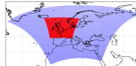
2.2 Regional Composition-Climate Model (RCCM) The RCCM, referred to as the HadGEM3-A “regional” (HadGEM3-RA) configuration, is described in detail in Moufouma-Okia and Jones (2015), and is also based on the GA3.0/GL3.0 configuration of HadGEM3 (Walters et al., 2011). The RCCM has a horizontal resolution of 0.44◦×0.44◦(roughly 50 km×50 km) with a domain cover-ing most of Europe and northern Africa (Fig. 1) and the same 63 vertical levels as the GCCM. The RCCM closely follows the GCCM configuration (Sect. 2.1), with the same dynami-cal solver, radiation, precipitation, and cloud (PC2) schemes. The same principal components are included: the UKCA-ExtTC chemistry model, the CLASSIC aerosol model, and the JULES land-surface model. The model dynamical time step was reduced to 12 min (20 min in GCCM) to account for the increase in resolution and shorter turnaround of dy-namical processes and interactions. The chemical time step is 5 min. Boundary conditions, used to drive the RCCM from the GCCM, will be discussed in Sect. 3.
2.3 AQUM
The final, high-resolution nest employed is the AQUM (Air Quality in the Unified Model) air quality forecast model. AQUM, like both the GCCM and the RCCM, is based on the
Figure 1.Nested modelling domains. The rectangular boundary of the figure is an extract of the GCCM (resolution 140 km) contain-ing the RCCM domain (resolution 50 km) plotted in blue and the AQUM domain (resolution 12 km) in red.
MetUM. AQUM has a horizontal resolution of 0.11◦×0.11◦ (approximately 12 km×12 km) on a “rotated pole” grid, covering the UK and nearby western Europe (see Fig. 1), with 38 vertical levels up to 39 km. The LBCs, provided by the RCCM, are on 63 levels but interpolated onto the 38 lev-els of AQUM. The dynamical and chemistry time steps are both 5 min.
The set-up of this model is described in detail in Savage et al. (2013) and uses the same parametrization schemes as the global and regional CCMs described above, apart from large-scale cloud, where AQUM uses the diagnostic cloud scheme as described by Smith (1990). As with the GCCM and RCCM, AQUM uses the CLASSIC aerosol scheme (Jones et al., 2001; Bellouin et al., 2011) and the UKCA model for its gas-phase chemistry. This helps to improve consistency between many aspects of the models. For ex-ample, large-scale and convective transport, boundary layer mixing, and wet and dry deposition are similar between all the nests. However, a different chemistry mechanism, the Re-gional Air Quality (RAQ) scheme, is used and the photolysis scheme also differs. Photolysis rates in AQUM are calculated with the Fast-J online photolysis scheme (Wild et al., 2000; O’Connor et al., 2014), which is coupled to the modelled liq-uid water and ice content, and sulfate aerosols at every time step.
The RAQ chemistry scheme pre-dates the ExtTC scheme and has been used in AQUM throughout its development and use as a forecast model. The experience developed with AQUM and the understanding of model performance es-tablished relies on the continuing use of this scheme and therefore we chose to retain this scheme for the final nest. The scheme has 40 transported species, 18 non-advected species, 116 gas-phase reactions, and 23 photolysis reac-tions; 16 of the transported species are emitted: nitrogen ox-ide (NO), methane (CH4), carbon monoxide (CO),
formalde-hyde (HCHO), ethane (C2H6), acetaldehyde (CH3CHO),
propane (C3H8), acetone (CH3COCH3), isoprene (C5H8),
(C3H6), butane (C4H10), toluene, and o-xylene. As was the
case in the GCCM and the RCCM, there is two-way cou-pling of oxidants between CLASSIC and the RAQ chemistry scheme. Further details of the RAQ scheme can be found in Savage et al. (2013).
A comparison of the MetUM settings for all three config-urations described above can be seen in Table A1.
3 Experimental set-up
In this section, a description of the experimental set-up for modelling present-day air quality using the configurations of MetUM is provided, covering meteorological lower bound-ary conditions, emissions, upper boundbound-ary conditions, and lateral boundary conditions.
3.1 Model simulations and model calibration
Both the GCCM and the RCCM were initialized using me-teorological fields from a pre-existing 20-year simulation of the standard HadGEM3 configuration. The simulations for both these model configurations cover a total period of 6 model years representative of the decade centred around the year 2000, for both meteorology and emissions. The first year is considered as an additional spin-up and the last 5 years are used in the analysis. The GCCM was used to produce the offline lateral boundary conditions (LBCs) at 6-hourly inter-vals to drive the RCCM, together with the emissions and up-per and lower boundary conditions described below. LBCs include meteorological drivers (3-D winds, air temperature, air density, Exner pressure, humidity, and cloudiness), impor-tant chemical tracers from UKCA-ExtTC (O3, NO, nitrogen
dioxide (NO2), HNO3, dinitrogen pentoxide (N2O5), H2O2,
CH4, CO, HCHO, C2H6, C3H8, CH3COCH3, and peroxy
acetyl nitrate (PAN)), gas-phase aerosol precursors (SO2,
DMS) and aerosols (dust, sulfate, nitrate, soot, FFOC, and BB) from CLASSIC. In turn, the RCCM produced meteoro-logical and composition LBCs required to drive the AQUM national-scale air quality model. Simulations with AQUM were initialized from the last month of the first year of the RCCM and were continued for 5 model years by applying the LBCs supplied by the RCCM offline at 6-hourly inter-vals. The chemical and aerosol species provided in the LBCs are dust, SO2, DMS, SO4, soot, OCFF, nitrate, O3, NO, NO2,
N2O5, HONO2, H2O2, CH4, CO, HCHO, C2H6, PAN, and
C3H8.
For lower boundary conditions the GCCM used monthly mean distributions of sea surface temperature (SST) and sea ice cover (SIC), derived for the present day (1995–2005) from transient coupled atmosphere–ocean simulations (Jones et al., 2011) of the HadGEM2-ES model (Collins et al., 2011). It should be pointed out here that the entire set-up is intended to represent a decadal climatological mean state of near present-day conditions encompassing the period from
1995 to 2005 and centred on the year 2000. This particu-larly applies to the meteorological drivers (sea surface tem-perature, SSTs, and sea ice cover) and the anthropogenic emissions of pollutants. The latter will be discussed in more detail in Sect. 3.2. The vegetation distribution for each of the simulations was prescribed using the simulated vegeta-tion averaged for the same decade from this transient cli-mate run, on which crop area, as given in the 5th Coupled Model Intercomparison Project (CMIP5) land use maps (Ri-ahi et al., 2007; Hurtt et al., 2011), was superimposed. The same present-day SST and SIC climatologies developed for the GCCM were regridded to the RCCM and the AQUM do-mains using a simple linear regridding algorithm.
The GCCM was calibrated against O3measurements from
the monitoring station located at Mace Head Atmospheric Research Station in western Ireland at 53.3◦N and 9.9◦W. It is part of the Automatic Urban and Rural Monitoring Net-work (AURN) which is run by a number of institutions co-ordinated by Defra. The Mace Head monitoring station is representative of rural background conditions. Model out-put has been compared to the annual cycle of monthly mean O3 which is based on a multi-year climatology of observed
near-surface O3 concentrations. The parameterized O3
sur-face dry deposition was used to perform the calibration as the model shows very high sensitivity to deposition. The model has been optimized to reproduce both the magnitude and sea-sonal cycle of O3at the Mace Head site in the global model
domain as closely as possible by varying the O3surface dry
deposition flux within its uncertainty limits. An increase in the O3 dry deposition by 20 % yielded the best agreement,
with respect to both O3 monthly mean surface
concentra-tion and seasonal cycle, with the observed climatology at the Mace Head station, which is representative of the O3
back-ground concentration in the lower troposphere, in the study area.
As the RCCM uses the same code base as the GCCM, this calibration is inherited by the former automatically. The model calibration has been applied to optimize consis-tency between the individual configurations in the global-to-national model nesting chain.
3.2 Emissions
A consistent set of emissions has been used for all three model configurations through using the same source data, but then regridding to the required resolution for each model.
The emissions of reactive gases and aerosols from anthro-pogenic and biomass burning sources used in this study are based on the dataset used for CMIP5 simulations and de-scribed by Lamarque et al. (2010). The models are all driven by decadal mean present-day emissions from CMIP5, repre-sentative of the decade centred on 2000. An example of the emissions for the different domains is given for NO in Fig. 2, while a full set of emission totals can be seen in Tables A2, A3, and A4.
UKCA-ExtTC takes into account emissions for 17 of its chemical species: nitrogen oxides (NOx=NO+NO2),
carbon monoxide (CO), hydrogen (H2), methanol,
formaldehyde, acetaldehyde and higher aldehydes, ace-tone (CH3COCH3), methyl ethyl ketone, ethane (C2H6),
propane (C3H8), butanes and higher alkanes, ethene, propene
and higher alkenes, isoprene, (mono)terpenes, and aromatic species. Of these butanes and higher alkanes, propene and higher alkenes, terpenes, and aromatics are treated as lumped species. Surface emissions are prescribed in most cases. The only exception is the emission of biogenic volatile organic compounds (BVOCs) which are calculated interactively in JULES using the iBVOC emission model (Pacifico et al., 2011). The emission of biogenic terpenes, methanol, and acetone follows the model described in Guenther et al. (1995). As summarized in Table A3, global annual total emissions of biogenic isoprene and monoterpenes interac-tively computed with the iBVOC model of, for instance, 480 Tg(C) yr−1 and of 95 Tg(C) yr−1 are in reasonably
good agreement with most other state-of-science interactive biogenic VOC emission models (e.g. Lathière et al., 2005; Guenther et al., 2006; Arneth et al., 2007; Müller et al., 2008; Messina et al., 2016) and global bVOC emission inventories (e.g. Arneth et al., 2008; Sindelarova et al., 2014). A detailed evaluation of the model performance is presented in Pacifico et al. (2011).
Emissions of NOx from lightning are taken into account
in UKCA. Lightning NOxemissions are calculated
interac-tively at every time step, based on the distribution and fre-quency of lightning flashes following Price and Rind (1992), Price and Rind (1993), and Price and Rind (1994). In this parametrization the lightning flash frequency is proportional to the height of the convective cloud top in all the models. For cloud-to-ground (CG) flashes lightning NOx emissions
are added below 500 hPa, distributed from the surface to the 500 hPa level, while NOxemissions resulting from
intra-cloud (IC) flashes are distributed from the 500 hPa level up to the convective cloud top. The emission magnitude is related to the discharge energy where CG flashes are 10 times more energetic than IC flashes (Price et al., 1997). The scheme im-plemented in the GCCM produces a total global emission
source of around 7 Tg(N) yr−1, which is in good agreement with the literature (cf. e.g. Schumann and Huntrieser, 2007). Soil-biogenic NOx emissions are taken from the monthly
mean distributions from the Global Emissions Inven-tory Activity (http://www.geiacenter.org/inventories/present. html), which are based on the global empirical model of soil-biogenic NOxemissions of Yienger and Levy II (1995)
giv-ing a global annual total of 5.6 Tg(N) yr−1.
For CH4, the UKCA model can be run by prescribing
surface emissions or prescribing either a constant or time-varying global mean surface concentration. For the simula-tions being evaluated here, a time-invariant CH4
concentra-tion of 1760 ppbv was prescribed at the surface.
The sea salt and mineral dust emissions are computed in-teractively at each model time step based on instantaneous near-surface wind speeds (Jones et al., 2001; Woodward, 2001). Mineral dust is a fully prognostic, advected species but, as mentioned in Sect. 2.1, sea salt is not advected and makes no contribution to model aerosol concentrations over land.
Similarly the ocean DMS emissions are computed based on wind speed, temperature, and climatological ocean DMS concentrations from Kettle et al. (1999), using the sea–air exchange flux scheme from Wanninkhof (1992).
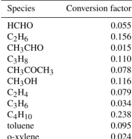
Emissions for AQUM are derived by re-gridding emis-sions from the regional model to the required 0.11◦ resolu-tion. The ExtTC and RAQ chemistry schemes emit different anthropogenic VOC species; consequently, some conversion is required. Our approach is to sum the anthropogenic VOC emission from ExtTC and apportion this total according to the values given in Table 1. These values were derived using the tabulated VOC emission fraction data over the UK for 2006 given by Dore et al. (2008). A consequence of this is that for some species the emission total in the smaller AQUM domain exceeds that of the larger RCCM domain. However, the total VOC emitted is conserved between AQUM and the corresponding part of the RCCM domain. For biogenic iso-prene emissions, AQUM uses an offline, monthly varying cli-matology which was derived from the online isoprene emis-sion fluxes generated by the RCCM. A diurnal cycle is ap-plied to account for daylight hours.
3.3 AQUM with higher-resolution emissions
Table 1.VOC split to convert total emitted VOCs from ExtTC to RAQ emitted VOCs. These factors sum to 1.0.
Species Conversion factor HCHO 0.055 C2H6 0.156
CH3CHO 0.015 C3H8 0.110
CH3COCH3 0.078 CH3OH 0.116
C2H4 0.079
C3H6 0.034
C4H10 0.238
toluene 0.095 o-xylene 0.024
the total emission has been rescaled to match the year 2000 decadal mean areal totals given by Lamarque et al. (2010) (as described in Sect. 3.2). For the remainder of the paper, this additional run will be referred to as AQUM-h.
3.4 Upper boundary conditions
While the chemistry is calculated interactively up to the model top in each configuration, upper boundary conditions are applied at the top of each model domain to account for missing stratospheric processes such as those related to CH4
oxidation and bromine and chlorine chemistry. These bound-ary conditions are described in detail in O’Connor et al. (2014) and are only briefly discussed here. For O3, the field
used in the radiation scheme by MetUM in the absence of interactive chemistry is used to overwrite the modelled O3
field in all model levels that are 3–4 km above the diag-nosed tropopause (Hoerling et al., 1993). For stratospheric odd nitrogen species (NOy), a fixed O3 to HNO3 ratio of
1.0/1000.0 kg(N)/kg(O3) from Murphy and Fahey (1994)
is applied to HNO3in the same vertical domain. Finally, for
CH4, an additional removal term is applied in the three
up-permost levels of the model. This CH4loss term was
calcu-lated in O’Connor et al. (2014) to be 50±10 TgCH4yr−1in
a global configuration.
4 Results
Our aim is to evaluate the air pollutant concentration out-put from the RCCM and AQUM simulations using different datasets representative of the true air quality in the UK. In this way, we also aim to assess the potential for improving modelled air pollutant concentrations by increasing model spatial resolution. The datasets we use include (i) in situ ob-servations of hourly air pollutant concentrations from the UK Automatic Urban and Rural Network (AURN) and (ii) an-nual mean surface pollutant concentrations produced by the Pollution Climate Mapping (PCM) model which also takes
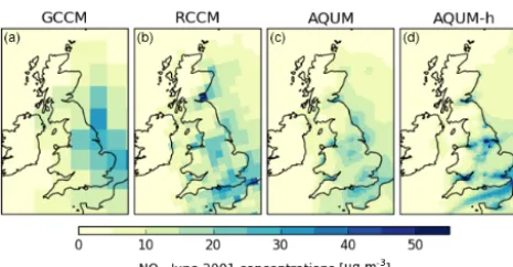
Figure 2.NO emissions for all models: GCCM(a), RCCM(b), AQUM(c), and the higher-resolution emissions run (AQUM-h)(d).
into account observations described by Brookes et al. (2013). This model produces gridded fields at a spatial resolution of 1 km over the whole of the UK.
Another aspect of the analysis undertaken is to employ two different approaches to model assessment. The first uses stan-dard verification metrics such as bias based on site-specific comparisons averaged over the 5-year modelled period. The second approach uses neighbourhood verification techniques which consider the area surrounding a particular point and thus allow for some mismatch in the spatial positioning of elevated pollutant values, thereby avoiding the well-known “double penalty” problem (Mittermaier, 2014).
We begin with a qualitative comparison of the GCCM against the two limited-area models in order to illustrate the need for improved resolution over that of the GCCM for air quality applications.
4.1 Comparison to GCCM
Figure 3 compares UK monthly mean NO2 concentrations
for June calculated from runs of the GCCM, RCCM, AQUM, and AQUM-h models. In the GCCM plot the resolution is wholly insufficient to realistically represent the elevated NO2
levels around the UK urban centres (London, West Midlands, Greater Manchester, West Yorkshire, Edinburgh) and in the busiest shipping lanes and ports (English Channel, Bristol Channel, Southampton, Liverpool). The representation im-proves qualitatively as we move to the right in this plot. It can clearly be seen that higher-resolution modelling is essen-tial for providing realistic pollutant representations at more localized spatial scales.
4.2 Comparison against in situ observations
Figure 3.Monthly mean NO2concentrations over the UK for June
for the four different model runs. From left to right: GCCM, RCCM, AQUM, AQUM-h.
Sects. 3.1 and 3.2, the simulations represent climatological mean states representative of the decade from 1995 to 2005 and centred on the year 2000. We compare the model to the AURN 2001–2005 observational record because it represents the most complete record for the selected period available. The individual model years do not correlate with the corre-sponding years in the observational record. We performed the multi-year simulations to obtain a statistical sample to inves-tigate interannual variability to some degree. The variability, of course, will be reduced due to the fact that composition and climate have been decoupled, but there is still variability in the atmospheric chemistry. From AURN we only consider “background” sites which include the site classifications of remote, rural, suburban, and urban background. We are there-fore excluding sites which we expect to be un-representative of a large area, such as roadside or industrial sites. As the models are driven by climatological meteorology, we do not expect the model results to match the hourly AURN obser-vations; hence, we compare values averaged over the 5-year period with corresponding averages derived from the hourly observations.
4.2.1 NO2
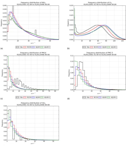
Figure 4a shows a frequency distribution of hourly ob-served concentrations of NO2with corresponding frequency
distributions for modelled concentrations from the RCCM, AQUM, and AQUM-h configurations. It is clear that the AQUM-h model distribution more closely matches the ob-served distribution than the other model configurations, il-lustrating the importance of increased spatial resolution and emissions for this pollutant. Corresponding statistical mea-sures of model skill are given in Table 2. The bias in RCCM and AQUM against AURN observations is−4.76 and
−5.47 µg m−3, respectively, but is reduced to−0.80 µg m−3 in AQUM-h. In Table 2 a comparison of the percentage of ob-servations/model values greater than the 65.0 µg m−3 thresh-old is also included; it illustrates that AQUM-h simulates ob-served frequencies of higher NO2concentrations well,
mak-ing it better suited to calculatmak-ing health burdens due to el-evated levels of NO2(e.g. Pannullo et al., 2017). However,
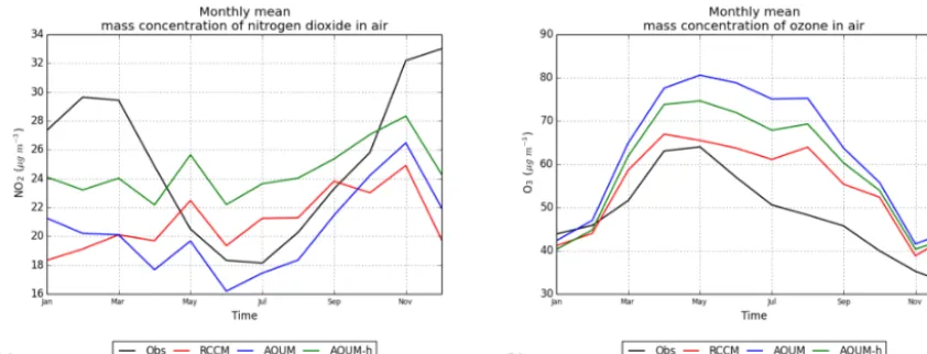
shown in Fig. 5a is a comparison of the seasonal cycle of ob-served and modelled NO2concentrations, averaged over all
AURN sites considered. This shows that none of the mod-els is able to fully capture the seasonal cycle of NO2, with
wintertime modelled concentrations biased low, while the RCCM and AQUM straddle the observed concentrations dur-ing summer. This is possibly due to the poor representation of the monthly variation of emissions over the UK in the global model which is then inherited by the higher resolution mod-els. However, other processes such as boundary layer mixing or chemistry could equally contribute. Further work would be required to elucidate this clearly.
4.2.2 O3
Relevant statistics are given in Table 2, while a frequency dis-tribution plot, showing the disdis-tribution of hourly O3
concen-trations over the entire period for models and observations, is shown in Fig. 4b and the seasonal cycle is given in Fig. 5b. The latter plot illustrates that the pattern of the seasonal cy-cle of O3 is captured reasonably well; however, the
mod-elled spring–summer maximum persists too long and does not replicate the gradual decline in monthly mean concen-trations as indicated by observations. This has implications for the use of modelled O3to quantify health impacts from
long-term exposure to O3 during warmer months, as
indi-cated by studies in North America (WHO, 2013b; COMEAP, 2015). In the frequency distribution plots in Fig. 4b, it can be seen that all models are able to reproduce the shape of the observed distribution quite well but differ in their most fre-quent concentration, corresponding to different model biases. The RCCM exhibits the smallest bias against observations of+6.23 µg m−3, and AQUM the greatest at+9.96 µg m−3 (see Table 2). However, the RCCM used an offline photol-ysis scheme (O’Connor et al., 2014), whilst both configu-rations of AQUM used the interactive Fast-J scheme (Wild et al., 2000). Given the different photolysis schemes used, a sensitivity experiment for a single month of July was carried out, in which AQUM-h was re-run with offline photolysis. The O3 bias for this month is 7.33 µg m−3 for the RCCM,
22.48 µg m−3 for AQUM, and 13.95 µg m−3 for AQUM-h. Although the photolysis rates relevant to O3,j(NO2)→NO,
and j(O3)→O1D are known to be biased low in the
of-fline photolysis scheme relative to both observations and online photolysis (Telford et al., 2013), the modelled O3
bias in AQUM-h is reduced to +6.99 µg m−3 with the
of-fline scheme, which is marginally better than the RCCM. However, the sensitivity of surface O3to the choice of
pho-tolysis scheme found here differs from two previous stud-ies (O’Connor et al., 2014; Telford et al., 2013). Both of these studies found that O3decreased in the Northern
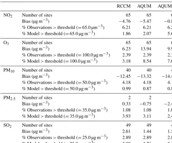
Table 2.Statistics comparing modelled air pollutant concentrations to AURN observations, for the period of the observational record 1 Jan-uary 2001–31 December 2005 (for the correlation between model years and the observational record compare the discussion in the text).
RCCM AQUM AQUM-h NO2 Number of sites 65 65 65
Bias (µg m−3) −4.76 −5.47 −0.80 % Observations>threshold (=65.0 µm−3) 6.21 6.21 6.21 % Model>threshold (=65.0 µg m−3) 1.86 2.07 5.64 O3 Number of sites 65 65 65
Bias (µg m−3) 6.23 13.94 9.96 % Observations>threshold (=100.0 µg m−3) 2.39 2.39 2.39 % Model>threshold (=100.0 µg m−3) 3.18 8.54 7.07 PM10 Number of sites 40 40 40
Bias (µg m−3) −12.45 −13.32 −14.41 % Observations>threshold (=50.0 µg m−3) 4.18 4.18 4.18 % Model>threshold (=50.0 µg m−3) 0.99 0.87 0.85 PM2.5 Number of sites 2 2 2
Bias (µg m−3) 0.33 −0.75 −2.46 % Observations>threshold (=35.0 µg m−3) 1.08 1.08 1.08 % Model>threshold (=35.0 µg m−3) 3.93 3.11 2.40 SO2 Number of sites 49 49 49 Bias (µg m−3) 2.61 1.44 1.59 % Observations>threshold (=25.0 µg m−3) 2.89 2.89 2.89 % Model>threshold (=25.0 µg m−3) 3.98 3.71 5.31
O3 budget were consistent between the two studies. In
ad-dition, O’Connor et al. (2014) found no significant change in modelled O3evident at NH mid-latitude sites (e.g. Mace
Head). However, both O’Connor et al. (2014) and Telford et al. (2013) were global studies rather than the regional scale considered here. Another conflicting factor is the cal-ibration which has been applied to the RCCM for the O3dry
deposition, which would have an impact on the O3
concen-trations, although this would have impacted AQUM through the LBCs. This calibration was not included in the papers de-scribed above, which may help to explain the conflicting re-sults. Consequently, these factors make it difficult to isolate and quantify the impact of the higher resolution third nest on model performance.
4.2.3 PM10
Relevant statistics are given in Table 2, while a frequency dis-tribution plot, showing the disdis-tribution of hourly PM10values
over the entire period for models and observations, is shown in Fig. 4c.
For PM10, none of the models are able to reproduce the
shape of the observed distribution, and there is a significant negative bias across all the model configurations (between
−12.45 and −14.41 µg m−3), with AQUM-h exhibiting the poorest performance. Poor modelling performance for PM10
is a common feature of many global composition and
re-gional air quality models (e.g. Colette et al., 2011; Im et al., 2015) and is often attributed to the unreliability of primary emissions of coarse component aerosol, both from anthro-pogenic and biogenic sources. In our simulations the lack of sea salt in modelled values over land points plays a signif-icant role in this underprediction. Putaud et al. (2010) esti-mate that over north-western Europe sea salt contributes on average between 7 % (kerbside sites) and 12 % (rural sites) of the observed annual mean PM10. In periods of strong winds
and at sites close to the coast downwind of the sea, values may be considerably higher. A related consequence of our lack of inclusion of sea salt is that our aerosol modelling does not include sodium nitrate, and so this coarse component of secondary aerosol is also missing from our estimates. These underpredictions could potentially affect the quantification of health effects due to short-term and long-term exposure of PM10, as documented by the WHO (2013b).
4.2.4 PM2.5
Relevant statistics are given in Table 2, while a frequency distribution plot, showing the distribution of hourly PM2.5
values over the entire period for models and observations, is shown in Fig. 4d.
For the finer PM2.5 component of aerosol, the
Figure 4.Frequency distribution of the main pollutants:(a)NO2,(b)O3,(c)PM10,(d)PM2.5, and(e)SO2. Observations are shown in black, RCCM in red, AQUM in blue, and AQUM-h in green.
positive bias for PM2.5 in the RCCM (+0.33 µg m−3),
whereas AQUM becomes slightly negative (−0.75 µg m−3)
and AQUM-h more negative still (−2.46 µg m−3).
However, the observed frequency distribution is only based on two background observational sites available for PM2.5 in the UK for the 2001–2005 time period. The
in-troduction of PM2.5monitoring stations in the UK increased
significantly from 2009 and we explored the possibility of
us-ing observations from 2011 to 2015 to generate a proxy for the 2001–2005 frequency distribution. However, we found that the PM10distribution changed significantly over the 10
years and concluded that it was not valid to use the more re-cent PM2.5observations in place of 2001–2005 observations.
Consequently, due to the paucity of PM2.5 observations for
Figure 5. Monthly mean concentrations of(a)NO2 and(b) O3. Observations are shown in black, RCCM in red, AQUM in blue, and
AQUM-h in green.
remainder of this paper, we shall no longer consider PM2.5
results.
4.2.5 SO2
Relevant statistics are given in Table 2, while a frequency dis-tribution plot, showing the disdis-tribution of hourly SO2values
over the entire period for models and observations, is shown in Fig. 4e.
For SO2, the model configurations exhibit similar
distri-butions to the observed distribution, with generally positive biases of between+1.44 and+2.61 µg m−3, with AQUM-h exhibiting the best performance.
4.3 Comparison against PCM
In order to assess the variation in the quality of modelled air pollutant concentrations between the different model config-urations, it is necessary to consider full spatial fields rather than the site comparison afforded by in situ observations de-scribed in the preceding section. Therefore, it is essential to compare the models against a realistic spatial field and, for this purpose, we use fields derived from the PCM model, as described in Brookes et al. (2013). This sophisticated model combines information from a variety of sources, including emission inventories and observation datasets, to produce es-timated annual mean surface pollutant concentrations on a 1 km×1 km grid over the entire UK for NO2, SO2, PM10,
and PM2.5. The data are freely available at https://uk-air.
defra.gov.uk/data/pcm-data. These results are widely used in the UK to provide the background pollutant concentrations for local air quality modelling studies and new site impact assessment studies. O3is also modelled by PCM, but the
out-put available is the number of days exceeding 120 µg m−3 (as required by the European Union ambient air quality directives (http://eur-lex.europa.eu/LexUriServ/LexUriServ. do?uri=OJ:L:2008:152:0001:0044:EN:PDF) rather than
pol-lutant concentrations, and so cannot be used in our analysis. In view of the lack of AURN PM2.5observations (also used
in deriving the PCM maps) during the period 2001–2005 (as described in Sect. 4.2.4), we have not considered PM2.5in
the following analysis.
PCM data for NO2 and PM10 are available for 2001–
2005, while SO2data are only available from 2002 onwards.
A comparison (not shown) of the PCM against the in situ AURN observations as done for the models in Sect. 4.2 proved the PCM verifies better than any of the other mod-els. PCM data from the available years were processed to produce 5-year means (4 years for SO2) for comparison with
the similarly averaged model fields.
Comparisons between MetUM modelled annual mean concentrations and PCM annual mean concentrations are shown for NO2, SO2, and PM10 in Fig. 6. In these plots
nearest neighbour regridding is used to interpolate the model fields and the PCM fields onto the 12 km AQUM grid. Spa-tial correlations have been calculated between the regridded model and PCM fields (only at valid PCM data points, i.e. UK land points) and are shown at the top of each figure.
For the primary pollutants of NO2 (Fig. 6a) and SO2
(Fig. 6b), there is an improvement in correlation with the PCM as we move from the RCCM to AQUM and finally AQUM-h: for NO2 the correlations are 0.822, 0.824, and
0.836, respectively, while for SO2the correlations are 0.664,
0.743, and 0.761, respectively. For SO2, the introduction or
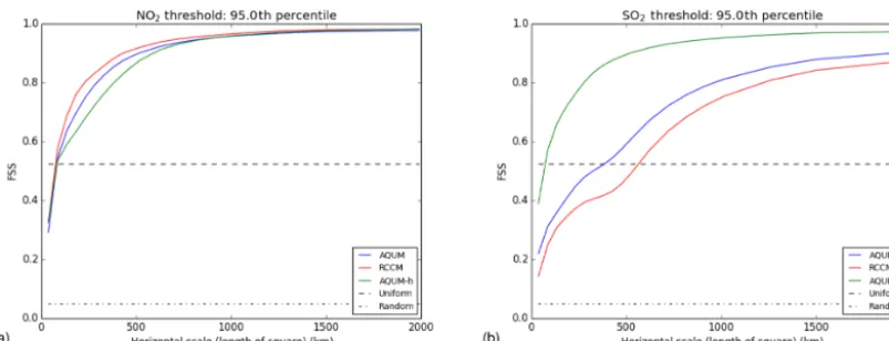
Figure 7.Fractional skill score for the 95th percentile for(a)NO2and(b)SO2. The RCCM is shown in red, AQUM in blue, and AQUM-h in
green. The “Random” (dot-dashed) line represents the FSS for a random forecast with the same fraction of points over the domain exceeding the percentile threshold as the truth field. The “Uniform” (dashed) line represents a forecast with the same fraction of points above the percentile threshold in the neighbourhood surrounding each grid point as the truth field for every grid point. Above this line the forecast is considered skilful.
the strongly inhomogeneous spatial distribution of these pol-lutants.
For PM10, however (Fig. 6c), this improvement in
correla-tion with higher resolucorrela-tion is not as clear. The correlacorrela-tion values with the PCM are 0.841 for the RCCM, 0.912 for AQUM, and 0.883 for AQUM-h. PM10has a large secondary
contribution which contributes a relatively smoothly varying background to the PCM maps in Fig. 6c. This is likely to be the reason for the lack of a clear improvement in PM10
modelling with the high-resolution AQUM-h model. Beyond the figures shown above, we also investigated the correlation scores by just considering data above fixed threshold concentration values (plots not shown). However, these results were very variable, depending on the thresh-old values considered, partly due to the biases (as given in Sect. 4.2).
4.4 Analyses based on neighbourhood comparisons: the fractional skill score
In evaluating a comparison of modelled air pollutant centrations against some gridded representation of true con-centrations (such as the PCM fields described above), small offsets in the spatial location of elevated values can give an exaggerated contribution to simple metrics such as bias and root mean square error evaluated at each grid point. This is commonly referred to as the “double penalty” problem. The resulting analysis may then give a misleading indica-tion of the comparison between the two fields. So-called “neighbourhood” verification techniques (Ebert, 2008; Mit-termaier, 2014) have been developed to avoid these prob-lems. Here, we consider the use of the fractional skill score (FSS) (explained in detail in Roberts and Lean, 2008) to analyse the variation in model skill in representing spatial patterns. This statistic has mainly been employed in
evalu-ating the improvements offered by high-resolution precipita-tion forecasts, where a “double penalty” problem occurs if rain is forecast in a neighbouring grid box to where it was actually observed (hence an incorrect forecast in both grid boxes). A lower resolution forecast might place the forecast and observed shower in the same grid box, resulting in an ap-parently improved forecast. Similar issues are found in pol-lution modelling due to the high degree of inhomogeneity of air pollutant concentrations and evaluation of the FSS may offer improved comparisons.
The FSS is calculated by computing, for each grid box, the fraction of neighbouring grid boxes which exceed a given threshold value (or percentile). This is done both for the grid-ded model fields that are to be evaluated and a gridgrid-ded bench-mark field representative of the “truth”, which in this case is the PCM fields, as described in Sect. 4.3. This can be re-peated for varying neighbourhood sizes. As the size of the neighbourhood increases, the fractional skill score should in-crease towards unity. A forecast may be considered “skilful” at the grid scale where the model has the correct fraction of points above the percentile threshold in the neighbourhood surrounding each grid point as the truth field for every grid point.
We have calculated the FSS using output from the three model configurations (RCCM, AQUM, and AQUM-h) and compared it to the PCM for various threshold values, based on both fixed thresholds and percentile values. An example set of results is shown in Fig. 7. In these plots, the varia-tion of FSS against the spatial scale is shown for the RCCM, AQUM, and AQUM-h, using a 95th percentile threshold. For NO2, there is little difference between the three model
con-figurations, and the same is found for PM10 (not shown).
SO2, AQUM-h shows the best performance, crossing the
threshold value of 0.5 at the shortest spatial scale, and reflects the strong point sources of SO2in contrast to NO2emissions.
The use of neighbourhood verification techniques to compare our different nests has therefore not offered any obvious in-creased insight into the differences between the models and the consequent impacts on improved predictions across the spatial scales. This may be an indication that the resolution differences between the models may not be the key factor in determining performance, particularly for NO2and PM10.
5 Summary and conclusions
This study describes the initial development of a more con-sistent framework for dynamic downscaling of climate and air quality from a global composition-climate model to the national scale, via a regional composition-climate model and thence to a higher-resolution regional air quality forecast model. In this attempt, some of the difficulties in presenting a clear-cut, quantitative demonstration of the value of higher resolution modelling have been made apparent. All three models use a single modelling framework – the MetUM – but some differences between the models do remain. The most notable of these are the different chemistry mechanisms, pho-tolysis schemes, and the calibration factor that have been used in the GCCM and RCCM compared to AQUM. AQUM has been developed with forecasting air quality over the UK as its primary aim, and performance has been optimized for predicting in situ UK observations on an hourly timescale with a focus on high impact, more extreme events. By con-trast, the GCCM and RCCM have been developed to predict global and regional climatologies, giving a faithful represen-tation of seasonal and annual means across the entire globe. These differences have resulted in some of the inconsisten-cies highlighted in this paper. This has led to a challenge in determining the benefits of a three-level nest for downscaling to the regional scale, but has highlighted important areas for consideration in future work.
The comparison of modelled air pollutant concentrations against in situ UK observations was conducted initially by a traditional site-specific analysis, with standard metrics such as bias. In addition, the impacts of model resolution on pollu-tant spatial patterns were assessed via comparison to the grid-ded PCM annual average pollution maps. In order to guard against the susceptibility of the traditional verification meth-ods to the double penalty problem, an analysis was also car-ried out using a neighbourhood approach, utilizing the frac-tional skill score (FSS), although the results from this were generally inconclusive.
For NO2, significantly improved modelled concentrations
can be quantitatively demonstrated for the higher-resolution models, using higher resolution emissions (biases of−4.76,
−5.47, and−0.80 µg m−3for RCCM, AQUM, and AQUM-h, respectively). This is readily understood, given the
depen-dence of surface concentrations of this primary pollutant on local emissions. For another primary pollutant, SO2, a
mod-est benefit of high-resolution modelling is demonstrated by the small increase in spatial correlation of AQUM-h with the PCM climatology maps (correlations compared to the PCM of 0.664, 0.743, and 0.761 for RCCM, AQUM, and AQUM-h). However, the benefit is less pronounced for SO2than for
NO2. The main reason for this is likely to be that in the UK,
SO2levels have fallen dramatically over the last 25 years and
ambient concentrations are now generally the result of rel-atively low magnitude traffic emissions and much stronger emissions from a small number of industrial point sources. This results in an annually averaged mean concentration map over the UK which shows relatively little spatial structure, but with a small number of locations having much higher concentrations due to strong local emission sources (see the PCM 1 km plot in Fig. 6b). This low level background with little overall spatial structure limits the quantitative increases in spatial correlation with the PCM climatologies. Another reason may be the impact of the introduction and removal of strong point emissions sources affecting the comparison, as noted in Sect. 4.3.
Conclusions regarding the benefits of high-resolution modelling for PM2.5have been hampered in the present study
due to the lack of observations over the study period. This pollutant has both primary and secondary contributions and one might expect improvements in the modelling of the pri-mary component by higher-resolution modelling. However, the magnitude of the improvement will depend on the relative sizes of primary and secondary components and it may well be that the contribution of the large secondary component masks any improvement in the representation of the primary component. For PM10, model performance remains poor
re-gardless of model resolution, with all three regional models (RCCM, AQUM, and AQUM-h) failing to capture the ob-served frequency distribution and having negative biases in the range−14.41 to−12.45 µg m−3. Based on the observed PM values analysed by Putaud et al. (2010), it is estimated that the lack of sea salt lowers the modelled PM10 annual
mean values by around 12 %. Additional important factors in the underprediction of PM10 magnitudes include the
ab-sence of coarse component sodium nitrate aerosol, the poor representation of other coarse component primary emissions, and poor modelling of the growth of aerosols to sizes in the coarse range.
For O3, all regional models were able to reproduce the
shape of the observation distribution well, but the offset of the modelled from the observed central location varied. Tests showed that the differences are likely to be largely due to differences in the photolysis schemes employed. However, given the modest benefits of higher-resolution modelling found for the other secondary pollutants, it seems unlikely that high-resolution modelling with AQUM would offer sig-nificantly improved performance for O3predictions beyond
The model simulations described in this paper have been evaluated in their air quality performance under present-day climate. However, the same techniques can be applied for projecting future climate and air quality from the global scale to the UK national scale (Folberth et al., 2017a). The ability to model air quality at the regional scale will be particularly important for health impact modelling where high spatial res-olution is important to allow the concentration variations to be matched to population locations. Indeed, the techniques in this paper have already been applied to 2050s climate and air quality in Pannullo et al. (2017) for assessing potential changes in UK hospital admissions.
Appendix A
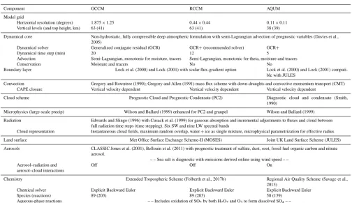
In Table A1 a summary of the parametrization schemes using the three model configurations is presented. Summaries of emission totals are given in Tables A2, A3, and A4.
Table A1.Summary of model configuration settings used in the GCCM, RCCM, and AQUM models.
Component GCCM RCCM AQUM
Model grid
Horizontal resolution (degrees) 1.875×1.25 0.44×0.44 0.11×0.11 Vertical levels (and top height, km) 63 (41) 63 (41) 38 (39)
Dynamical core Non-hydrostatic, fully compressible deep atmospheric formulation with semi-Lagrangian advection of prognostic variables (Davies et al., 2005)
Dynamical solver Generalized conjugate residual (GCR) GCR+(recommended solver) GCR+
Dynamical time step (min) 20 12 5
Advection Semi-Lagrangian, monotonic for moisture, tracers Semi-Lagrangian, monotonic for theta, moisture and tracers
Conservation Moisture and tracers No No
Boundary layer Lock et al. (2000) and Lock (2001) with scalar flux-gradient option Lock et al. (2000) and Lock (2001) compati-ble with JULES
Convection Gregory and Rowntree (1990); Gregory and Allen (1991) mass flux scheme with down-draughts and convective momentum transport (CMT) CAPE closure Vertical velocity dependent Vertical velocity dependent Vertical velocity dependent
Cloud scheme Prognostic Cloud and Prognostic Condensate (PC2) Diagnostic cloud and condensate (Smith, 1990)
Microphysics (large-scale precip) Wilson and Ballard (1999) enhanced for PC2 and graupel Wilson and Ballard (1999)
Radiation Edwards and Slingo (1996) with Cusack et al. (1999) for gaseous absorption and incremental adjustments to fluxes and cloud between full radiation time steps (time stepping). Six SW and nine LW spectral bands
Cloud representation Instantaneous cloud fields, maximum random overlap, water+ice as single mixture, microphysical parametrization for effective radius
Land surface Met Office Surface Exchange Scheme-II (MOSES) Joint UK Land Surface Scheme (JULES)
Aerosols CLASSIC Jones et al. (2001), Bellouin et al. (2011) with prognostic treatment of sulfate, dust, soot, fossil fuel organic carbon and nitrate aerosol.
– – Sea salt is diagnostic with emissions derived online using wind speed – – Aerosol–radiation and
aerosol–cloud interactions
Off Off On
Chemistry Extended Tropospheric Scheme (Folberth et al., 2017b) Regional Air Quality Scheme (Savage et al., 2013)
Chemical solver Explicit Backward Euler Explicit Backward Euler Explicit Backward Euler
Species (reactions) 89 (203) 89 (203) 58 (139)
Aqueous-phase reactions – – Includes oxidation of SO2by both H2O2and O3to form dissolved SO4– –
Photolysis scheme Offline, 2-Dimensional model with prescribed cloud and aerosol Fast-J, uses online cloud and aerosol
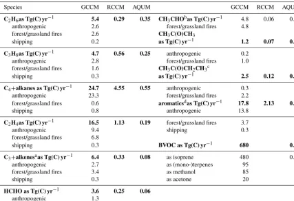
Table A2.Summary of the annual total emissions of trace gases used in the GCCM, RCCM, and AQUM models. Bold type shows the annual total for each species.
Species GCCM RCCM AQUM
NOxas Tg(N) yr−1 49.4 8.10 2.31
anthropogenic 26.5 forest/grassland fires 4.3 shipping 5.5
soil 5.6
lightning 7.5
CO as Tg(CO) yr−1 1112.8 83.93 20.23
anthropogenic 607.5 forest/grassland fires 459.1 shipping 1.2 oceanic 45.0
CH4as ppbv∗ 1760 1760 1760
H2as Tg(H2)yr−1 28.9 0.61 0.055
forest/grassland fires 28.9
∗ACH
Table A3.Summary of the annual total emissions of volatile organic compounds used in the GCCM, RCCM, and AQUM models. Bold type shows the annual total for each species.
Species GCCM RCCM AQUM GCCM RCCM AQUM
C2H6as Tg(C) yr−1 5.4 0.29 0.35 CH3CHObas Tg(C) yr−1 4.8 0.06 0.02
anthropogenic 2.6 forest/grassland fires 4.8
forest/grassland fires 2.6 CH3C(O)CH3
shipping 0.2 as Tg(C) yr−1 1.2 0.07 0.14
C3H8as Tg(C) yr−1 4.7 0.56 0.25 anthropogenic 0.2
anthropogenic 2.8 forest/grassland fires 1.0
forest/grassland fires 1.6 CH3C(O)CH2CH3c
shipping 0.3 as Tg(C) yr−1 2.5 0.12 0.00
C4+alkanes as Tg(C) yr−1 24.7 4.55 0.55 anthropogenic 0.3
anthropogenic 23.3 forest/grassland fires 2.2
forest/grassland fires 0.6 aromaticsdas Tg(C) yr−1 17.8 2.13 0.30
shipping 0.8 anthropogenic 13.8
C2H4as Tg(C) yr−1 16.5 1.13 0.19 forest/grassland fires 3.7
anthropogenic 9.4 shipping 0.3
forest/grassland fires 6.8
shipping 0.3 BVOC as Tg(C) yr−1 680 0.87
C3+alkenesaas Tg(C) yr−1 6.4 0.33 0.08 as isoprene 480 0.87
anthropogenic 2.7 as (mono-)terpenes 95 0
forest/grassland fires 3.4 as methanol 85 0
shipping 0.3 as acetone 20 0
HCHO as Tg(C) yr−1 3.6 0.25 0.06
anthropogenic 1.3
forest/grassland fires 2.3
The method for deriving AQUM emissions of VOCs from RCCM emissions is described in Sect. 3.2 and involves partitioning the total VOC in the RCCM amongst the different VOC species in AQUM according to Table 1. As a consequence it is possible for emissions of some individual species in the smaller AQUM domain to exceed those in the larger RCCM domain, but the total VOC emitted is conserved.
aIncludes C
3plus higher alkenes and all volatile alkynes;bincludes higher aldehydes;cincludes methyl ethyl ketone (MEK) plus higher ketones;dincludes
benzene, toluene, and xylenes.
Table A4.Summary of the annual total emissions of aerosols used in the GCCM, RCCM, and AQUM models. Bold type shows the annual total for each species.
Species GCCM RCCM AQUM
black carbon (BC) as Tg(BC) yr−1 6.4 0.87 0.23
anthropogenic 6.4
shipping 0.03
organic carbon (OC) as Tg(OC) yr−1 24.3 1.84 0.23
anthropogenic 23.6
shipping 0.7
NH3as Tg(N) yr−1 35.4 6.98 1.67
anthropogenic 32.8 forest/grassland fires 2.6
SO2as Tg(SO2) yr−1 107.3 22.61 1.90
anthropogenic 87.6 forest/grassland fires 12.2
Competing interests. The authors declare that they have no conflict of interest.
Acknowledgements. The development of HadGEM3, UKCA, and the work of Mohit Dalvi, Gerd Folberth, and Fiona M. O’Connor were supported by the Joint UK BEIS/Defra Met Office Hadley Centre Climate Programme (GA01101). Lucy S. Nea, Mohit Dalvi, Gerd Folberth, Rachel N. McInnes, and Paul Agnew also acknowl-edge the Engineering and Physical Sciences Research Council (EPSRC) for additional funding through the UK Engineering and Physical Sciences research council grant number EP/J017485/1: “A rigorous statistical framework for estimating the long-term health effects of air pollution”. In addition, this work and its contributors (GF and FMO’C) were partly supported by the UK-China Research & Innovation Partnership Fund through the Met Office Climate Science for Service Partnership (CSSP) China as part of the Newton Fund.
Edited by: Olaf Morgenstern
Reviewed by: two anonymous referees
References
Allen, R. J., Landuyt, W., and Rumbold, S. T.: An in-crease in aerosol burden and radiative effects in a warmer world, Nat. Clim. Chang., 6, 269–274, https://doi.org/10.1038/NCLIMATE2827, 2016.
Arneth, A., Niinemets, Ü., Pressley, S., Bäck, J., Hari, P., Karl, T., Noe, S., Prentice, I. C., Serça, D., Hickler, T., Wolf, A., and Smith, B.: Process-based estimates of terrestrial ecosys-tem isoprene emissions: incorporating the effects of a di-rect CO2-isoprene interaction, Atmos. Chem. Phys., 7, 31–53, https://doi.org/10.5194/acp-7-31-2007, 2007.
Arneth, A., Monson, R. K., Schurgers, G., Niinemets, Ü., and Palmer, P. I.: Why are estimates of global terrestrial isoprene emissions so similar (and why is this not so for monoterpenes)?, Atmos. Chem. Phys., 8, 4605–4620, https://doi.org/10.5194/acp-8-4605-2008, 2008.
Ashworth, K., Folberth, G., Hewitt, C. N., and Wild, O.: Impacts of near-future cultivation of biofuel feedstocks on atmospheric composition and local air quality, Atmos. Chem. Phys., 12, 919– 939, https://doi.org/10.5194/acp-12-919-2012, 2012.
Baklanov, A., Schlünzen, K., Suppan, P., Baldasano, J., Brunner, D., Aksoyoglu, S., Carmichael, G., Douros, J., Flemming, J., Forkel, R., Galmarini, S., Gauss, M., Grell, G., Hirtl, M., Joffre, S., Jorba, O., Kaas, E., Kaasik, M., Kallos, G., Kong, X., Ko-rsholm, U., Kurganskiy, A., Kushta, J., Lohmann, U., Mahura, A., Manders-Groot, A., Maurizi, A., Moussiopoulos, N., Rao, S. T., Savage, N., Seigneur, C., Sokhi, R. S., Solazzo, E., Solomos, S., Sørensen, B., Tsegas, G., Vignati, E., Vogel, B., and Zhang, Y.: Online coupled regional meteorology chemistry models in Europe: current status and prospects, Atmos. Chem. Phys., 14, 317–398, https://doi.org/10.5194/acp-14-317-2014, 2014. Bellouin, N., Rae, J., Jones, A., Johnson, C., Haywood, J., and
Boucher, O.: Aerosol forcing in the Climate Model Intercompar-ison Project (CMIP5) simulations by HadGEM2-ES and the role
of ammonium nitrate, J. Geophys. Res.-Atmos., 116, D20206, https://doi.org/10.1029/2011JD016074, 2011.
Best, M. J., Pryor, M., Clark, D. B., Rooney, G. G., Essery, R. L. H., Ménard, C. B., Edwards, J. M., Hendry, M. A., Porson, A., Gedney, N., Mercado, L. M., Sitch, S., Blyth, E., Boucher, O., Cox, P. M., Grimmond, C. S. B., and Harding, R. J.: The Joint UK Land Environment Simulator (JULES), model description – Part 1: Energy and water fluxes, Geosci. Model Dev., 4, 677–699, https://doi.org/10.5194/gmd-4-677-2011, 2011.
Boucher, O., Randall, D., Artaxo, P., Bretherton, C., Feingold, G., Forster, P., Kerminen, V.-M., Kondo, Y., Liao, H., Lohmann, U., Rasch, P., Satheesh, S., Sherwood, S., Stevens, B., and Zhang, X.: Clouds and Aerosols, book section 7, 571–658, Cambridge University Press, Cambridge, UK and New York, NY, USA, https://doi.org/10.1017/CBO9781107415324.016, 2013. Brookes, M. D., Stedman, J. R., Kent, A. J., Morris, R. J., Cooke,
S. L., Lingard, J. J. N., Rose, R. A., Vincent, K. J., Bush, T. J., and Abbott, J.: Technical report on UK supplementary assessment under the Air Quality Directive(2008/50/EC), the Air Quality Framework Directive(96/62/EC) and Fourth Daughter Directive(2004/107/EC) for 2012, Tech. rep., The Department for Environment, Food and Rural Affairs, Welsh Government, the Scottish Government and the De-partment of the Environment for Northern Ireland, available at: http://uk-air.defra.gov.uk/assets/documents/reports/cat09/ 1312231525_AQD_DD4_2012mapsrepv0.pdf (last access: 23 October 2017), 2013.
Brown, A., Milton, S., Cullen, M., Golding, B., Mitchell, J., and Shelly, A.: Unified Modeling And Prediction Of Weather And Climate A 25-Year Journey, B. Am. Meteorol. Soc., 93, 1865– 1877, 2012.
Chemel, C., Fisher, B., Kong, X., Francis, X., Sokhi, R., Good, N., Collins, W., and Folberth, G.: Application of chemical transport model CMAQ to policy decisions re-garding PM2.5 in the UK, Atmos. Environ., 82, 410–417, https://doi.org/10.1016/j.atmosenv.2013.10.001, 2014.
Colette, A., Granier, C., Hodnebrog, Ø., Jakobs, H., Maurizi, A., Nyiri, A., Bessagnet, B., D’Angiola, A., D’Isidoro, M., Gauss, M., Meleux, F., Memmesheimer, M., Mieville, A., Rouïl, L., Russo, F., Solberg, S., Stordal, F., and Tampieri, F.: Air quality trends in Europe over the past decade: a first multi-model assessment, Atmos. Chem. Phys., 11, 11657–11678, https://doi.org/10.5194/acp-11-11657-2011, 2011.
Collins, W. J., Bellouin, N., Doutriaux-Boucher, M., Gedney, N., Halloran, P., Hinton, T., Hughes, J., Jones, C. D., Joshi, M., Lid-dicoat, S., Martin, G., O’Connor, F., Rae, J., Senior, C., Sitch, S., Totterdell, I., Wiltshire, A., and Woodward, S.: Development and evaluation of an Earth-System model – HadGEM2, Geosci. Model Dev., 4, 1051–1075, https://doi.org/10.5194/gmd-4-1051-2011, 2011.
COMEAP: Quantification of mortality and hospital admissions as-sociated with ground-level ozone, Committee on the Medical Effects of Air Pollutants, UK, available at: https://www.gov. uk/government/collections/comeap-reports (last access: 23 Oc-tober 2017), 2015.
Davies, T., Cullen, M. J. P., Malcolm, A. J., Mawson, M. H., Staniforth, A., White, A. A., and Wood, N.: A new dynam-ical core for the Met Office’s global and regional modelling of the atmosphere, Q. J. Roy. Meteor. Soc., 131, 1759–1782, https://doi.org/10.1256/qj.04.101, 2005.
Dore, C. J., Murrells, T. P., Passant, N. R., Hobson, M. M., Thistlethwaite, G., Wagner, A., Li, Y., Bush, T., King, K. R., Norris, J., Coleman, P. J., Walker, C., Stewart, R. A., Tsagatakis, I., Conolly, C., Brophy, N. C. J., and Hann, M. R.: UK Emissions of Air Pollutants 1970 to 2006, Tech. rep., AEA, available at: http://uk-air.defra.gov.uk/reports/cat07/ 0810291043_NAEI_2006_Report_Final_Version(3).pdf (last ac-cess: 23 October 2017), 2008.
Ebert, E. E.: Fuzzy verification of high-resolution gridded forecasts: a review and proposed framework, Meteorol. Appl., 15, 51–64, https://doi.org/10.1002/met.25, 2008.
Edwards, J. M. and Slingo, A.: Studies with a flexible new radiation code. I: Choosing a configuration for a large-scale model, Q. J. Roy. Meteor. Soc., 122, 689–719, https://doi.org/10.1002/qj.49712253107, 1996.
Eyring, V., Arblaster, J. M., Cionni, I., Sedlacek, J., Perliwitz, J., Young, P. J., Bekki, S., Bergmann, D., Cameron-Smith, P., Collins, W. J., Faluvegi, G., Gottschaldt, K. D., Horowitz, L. W., Kinnison, D. E., Lamarque, J. F., Marsh, D. R., Saint-Martin, D., Shindell, D. T., Sudo, K., Szopa, S., and Watanabe, S.: Long-term ozone changes and associated climate impacts in CMIP5 simulations, J. Geophys. Res.-Atmos., 118, 5029–5060, https://doi.org/10.1002/jgrd.50316, 2013.
Fiore, A. M., Naik, V., Spracklen, D. V., Steiner, A., Unger, N., Prather, M., Bergmann, D., Cameron-Smith, P. J., Cionni, I., Collins, W. J., Dalsoren, S., Eyring, V., Folberth, G. A., Ginoux, P., Horowitz, L. W., Josse, B., Lamarque, J.-F., MacKenzie, I. A., Nagashima, T., O’Connor, F. M., Righi, M., Rumbold, S. T., Shindell, D. T., Skeie, R. B., Sudo, K., Szopa, S., Takemura, T., and Zeng, G.: Global air quality and climate, Chem. Soc. Rev., 41, 6663–6683, https://doi.org/10.1039/c2cs35095e, 2012. Folberth, G., McInnes, R. N., Dalvi, M., Neal, L. S., Agnew, P.,
Clewlow, Y., Hemming, D., O’Connor, F., and Sarran, C.: Fu-ture projections of UK air quality and potential implications for health, in preparation, 2017a.
Folberth, G. A., Abraham, N. L., Johnson, C. E., Morgenstern, O., O’Connor, F. M., Pacifico, F., Young, P. A., Collins, W. J., and Pyle, J. A.: Evaluation of the new UKCA climate-composition model. Part III. Extension to tropospheric chemistry and biogeo-chemical coupling between atmosphere and biosphere, in prepa-ration, 2017b.
Forkel, R. and Knoche, R.: Regional climate change and its impact on photooxidant concentrations in southern Germany: Simulations with a coupled regional climate-chemistry model, J. Geophys. Res.-Atmos., 111, D12302, https://doi.org/10.1029/2005JD006748, 2006.
Gregory, D. and Allen, S.: The effect of convective downdraughts upon NWP and climate simulations, 122–123, Nineth conference on numerical weather prediction, Denver, Co1orado, 1991. Gregory, D. and Rowntree, P. R.: A mass flux convection
scheme with representation of cloud ensemble charac-teristics and stability-dependent closure, Mon. Weather Rev., 118, 1483–1506, https://doi.org/10.1175/1520-0493(1990)118<1483:AMFCSW>2.0.CO;2, 1990.
Grell, G., Peckham, S., Schmitz, R., McKeen, S., Frost, G., Skamarock, W., and Eder, B.: Fully coupled “online” chem-istry within the WRF model, Atmos. Environ., 39, 6957–6975, https://doi.org/10.1016/j.atmosenv.2005.04.027, 2005.
Guenther, A., Hewitt, C. N., Erickson, D., Fall, R., Geron, C., Graedel, T., Harley, P., Klinger, L., Lerdau, M., Mckay, W. A., Pierce, T., Scholes, B., Steinbrecher, R., Tallamraju, R., Taylor, J., and Zimmermann, P.: A global model of natural volatile or-ganic compound emissions, J. Geophys. Res., 100, 8873–8892, 1995.
Guenther, A., Karl, T., Harley, P., Wiedinmyer, C., Palmer, P. I., and Geron, C.: Estimates of global terrestrial isoprene emissions using MEGAN (Model of Emissions of Gases and Aerosols from Nature), Atmos. Chem. Phys., 6, 3181–3210, https://doi.org/10.5194/acp-6-3181-2006, 2006.
He, J., Zhang, Y., Glotfelty, T., He, R., Bennartz, R., Rausch, J., and Sartelet, K.: Decadal simulation and comprehensive evalua-tion of CESM/CAM5.1 with advanced chemistry, aerosol micro-physics, and aerosol-cloud interactions, J. Adv. Model. Earth Sy., 7, 110–141, https://doi.org/10.1002/2014MS000360, 2015. Heal, M. R., Heaviside, C., Doherty, R. M., Vieno, M., Stevenson,
D. S., and Vardoulakis, S.: Health burdens of surface ozone in the UK for a range of future scenarios, Environ. Int., 61, 36–44, https://doi.org/10.1016/j.envint.2013.09.010, 2013.
Hoerling, M. P., Schaack, T. K., and Lenzen, A. J.: A Global Analysis of Stratospheric–Tropospheric Exchange during Northern Winter, Mon. Weather Rev., 121, 162–172, https://doi.org/10.1175/1520-0493(1993)121<0162:AGAOSE>2.0.CO;2, 1993.
Hong, C., Zhang, Q., Zhang, Y., Tang, Y., Tong, D., and He, K.: Multi-year downscaling application of two-way cou-pled WRF v3.4 and CMAQ v5.0.2 over east Asia for re-gional climate and air quality modeling: model evaluation and aerosol direct effects, Geosci. Model Dev., 10, 2447–2470, https://doi.org/10.5194/gmd-10-2447-2017, 2017.
Hough, A.: The calculation of photolysis rates for use in global tro-pospheric modelling studies, Tech. Rep. 13259, Atomic Energy Research Establishment, Harvel, UK, 1988.
Hurrell, J. W., Holland, M. M., Gent, P. R., Ghan, S., Kay, J. E., Kushner, P. J., Lamarque, J.-F., Large, W. G., Lawrence, D., Lindsay, K., Lipscomb, W. H., Long, M. C., Mahowald, N., Marsh, D. R., Neale, R. B., Rasch, P., Vavrus, S., Vertenstein, M., Bader, D., Collins, W. D., Hack, J. J., Kiehl, J., and Mar-shall, S.: The Community Earth System Model: a framework for collaborative research, B. Am. Meteorol. Soc., 94, 1339–1360, https://doi.org/10.1175/BAMS-D-12-00121.1, 2013.