Homogenization of Portuguese long-term temperature data series: Lisbon, Coimbra and Porto

Earth Syst. Sci. Data, 4, 187–213, 2012 www.earth-syst-sci-data.net/4/187/2012/ doi:10.5194/essd-4-187-2012

©Author(s) 2012. CC Attribution 3.0 License.

History

Geo- and Space

Sciences

Open

Access

Advances

Science & Research

Open Access Proceedings

Open Access Earth System

Science

Data

Science

Data

Drinking Water

Open Access

Drinking Water

Discussions O pen Acc es s

Social

Geography

Social

Geography

Homogenization of Portuguese long-term temperature

data series: Lisbon, Coimbra and Porto

A. L. Morozova1and M. A. Valente2

1_{Centro de Geof´ısica da Universidade de Coimbra, University of Coimbra, Portugal} 2_{Instituto Dom Luiz, University of Lisbon, Portugal}

Correspondence to: A. L. Morozova (anna m@teor.fis.uc.pt)

Received: 21 June 2012 – Published in Earth Syst. Sci. Data Discuss.: 25 July 2012 Revised: 13 November 2012 – Accepted: 14 November 2012 – Published: 14 December 2012

Abstract. Three long-term temperature data series measured in Portugal were studied to detect and correct

non-climatic homogeneity breaks and are now available for future studies of climate variability.

Series of monthly minimum (Tmin) and maximum (Tmax) temperatures measured in the three Portuguese

mete-orological stations of Lisbon (from 1856 to 2008), Coimbra (from 1865 to 2005) and Porto (from 1888 to 2001) were studied to detect and correct non-climatic breaks. These series, together with monthly series of average temperature (Taver) and temperature range (DTR) derived from them, were tested in order to detect breaks,

using firstly metadata, secondly a visual analysis, and thirdly four widely used homogeneity tests: von Neu-mann ratio test, Buishand test, standard normal homogeneity test, and Pettitt test. The homogeneity tests were used in absolute (using temperature series themselves) and relative (using sea-surface temperature anomalies series obtained from HadISST2.0.0.0 close to the Portuguese coast or already corrected temperature series as reference series) modes. We considered the Tmin, Tmaxand DTR series as most informative for the detection of

breaks due to the fact that Tminand Tmaxcould respond differently to changes in position of a thermometer or

other changes in the instrument’s environment; Taverseries have been used mainly as control.

The homogeneity tests showed strong inhomogeneity of the original data series, which could have both in-ternal climatic and non-climatic origins. Breaks that were identified by the last three mentioned homogeneity tests were compared with available metadata containing data such as instrument changes, changes in station location and environment, observation procedures, etc. Significant breaks (significance 95 % or more) that coincided with known dates of instrumental changes were corrected using standard procedures. It was also noted that some significant breaks, which could not be connected to known dates of any changes in the park of instruments or stations location and environment, were probably caused by large volcanic eruptions. The corrected series were again tested for homogeneity; the corrected series were considered free of non-climatic breaks when the tests of most of monthly series showed no significant (significance 95 % or more) breaks that coincide with dates of known instrument changes. Corrected series are now available within the framework of ERA-CLIM FP7 project for future studies of climate variability (doi:10.1594/PANGAEA.785377).

1 Introduction

Long instrumental climatological records assume a paramount role in the studies of variation of the atmo-spheric conditions. They provide vital information about climate variability, trends and cycles. Unfortunately, long-term series often contain inhomogeneities caused by a

detected and corrected beforehand, and only after that could the data series be used in any kind of climate studies.

The problem of identification and correction of non-climatic inhomogeneities has been studied thoroughly (see, e.g. review in Peterson et al., 1998). The simplest way to de-tect the shift-like inhomogeneities is a visual analysis, prefer-ably by an experienced meteorologist (Peterson et al., 1998). It is clear that this method is very subjective and could be used as an initial part of the analysis, providing information about “doubtful” periods that have to be studied thoroughly with other objective methods.

At the moment, there exist a lot of objective statistical methods accepted by the scientific community that can detect the presence and probable date of inhomogeneities, and new methods continue to be developed (see e.g. Venema et al., 2012). Most of these methods belong to one of three groups: likelihood-based methods, linear-regression based methods, and non-parametric methods (Wang et al., 2007). In cli-mate studies, the most commonly used methods are the stan-dard normal homogeneity test (SNHT; Alexandersson and Moberg, 1997) and its variations, the Buishand cumulative deviation test (Buishand, 1982), the non-parametric rank Pet-titt test (PetPet-titt, 1979), the two-phase regression methods (e.g. Solow, 1987) and others. These methods estimate not only the level of inhomogeneity of the tested series, but also de-tect the highly probable homogeneity break points (hereafter: breaks). The other tests, like the von Neumann ratio test (von Neumann, 1941), do not give any information about the date of the break, but estimate the overall level of inhomogeneity in the data.

The tasks of non-climatic breaks correction are compli-cated by the fact that not all inhomogeneities existing in data series are of non-climatic origin. There are breaks that origi-nate from “real” climate changes, like volcanic aerosol ejec-tions or abrupt changes of atmospheric and/or oceanic circu-lation. The non-climatic inhomogeneities have to be some-how separated from the others, and this task could be done using the metadata – a record of station relocations, changes in station environment, changes in the instrument park, ob-servation routines, applications of new formulae to calcu-late means, etc. The metadata could provide precise infor-mation about the dates and reasons for non-climatic changes and consequently ideal for use in any homogenization proce-dure. Moreover, all available information about stations’ his-tory should be preferred over statistical methods, especially in the tasks of detection of the breaks dates (Venema et al., 2012). Any break detected by statistical methods had to be checked against metadata, and if there is a written note that some intervention took place in the station setup at the break date, this break should be considered as non-climatic and (in most cases) be corrected (Peterson et al., 1998; Aguilar et al., 2003).

The analysis of the separate monthly series could provide different break points for each month, both due to the ran-domness of the meteorological time series and to the fact

that some inhomogeneities could have larger effect during the warm part of the year than during the cold part. Therefore, not only annual but also monthly (or seasonal) means have to be analysed in the process of homogenization (Aguilar et al., 2003).

The detected non-climatic inhomogeneities required cor-rection. The correction procedure was constructed so that all data were corrected in line with the conditions of the last ho-mogeneous part of the data series: a period ranging from the last break to the end of the series. In this case, all future peri-ods of the incoming data would not damage the homogeneity of the data series (Aguilar et al., 2003). The procedure of cor-rection is applied to the data series backward in time, start-ing from the most recent break. The most usual way to cor-rect non-climatic breaks is to calculate the means of the stud-ied parameter during some time before and after each of the breaks. The adjustment value is then a difference (or ratio in case of parameters like precipitation) between these means. Accordingly, the adjustment value is applied to the inhomo-geneous part (part before the break) of the series (Aguilar et al., 2003).

2 Methods for detection and correction of

non-climatic breaks

2.1 Homogeneity tests

Despite the fact that the main role in the detection of the breaks was assigned in this study to the metadata, four sim-ple, widely used statistical homogeneity tests were applied to the data (Klein Tank, 2007): von Neumann ratio test, Buis-hand test, standard normal homogeneity test (SNHT), and Pettitt test. The first test allows one to estimate only the pres-ence of breaks in the dataset, whereas the last three tests also give information about the possible dates of such breaks. The use of tests of different types (parametric, non-parametric, likelihood), which also have different sensitivities in diff er-ent parts of the series, could help to obtain more significant results.

Table 1.The 90 %, 95 % and 99 % critical values for the following homogeneity test statistics: N of the von Neumann ratio test, T0of the SNHT, XKof the Pettitt test and Q of the Buishand partial sum tests, for data sets with different lengths (114, 141 and 153 elements).

Test 114 141 153

90 % 95 % 99 % 90 % 95 % 99 % 90 % 95 % 99 %

von Neumann (N) 1.76 1.7 1.57 1.79 1.72 1.61 1.79 1.74 1.63

SNHT (T0) 7.9 9.3 12.4 8.0 9.5 12.6 8.1 9.5 12.7

Pettitt (XK) 757 864 1071 1041 1187 1472 1176 1341 1663

Buishand (Q) 12.5 13.8 16.5 14.0 15.3 18.3 14.6 15.9 19.0

2.1.1 Von Neumann ratio test – non-parametric test

In this test the null hypothesis is that the data are indepen-dent iindepen-dentically distributed random values; the alternative hy-pothesis is that the values in the series are not randomly dis-tributed. The von Neumann ratio N is defined as the ratio of the mean square successive (year to year) difference to the variance (von Neumann, 1941):

N=Xn−1

i=1(Yi−Yi+1) 2Xn

i=1

Yi−Y 2

. (1)

Hereafter, for each of the test descriptions, n is the data set length, Yiis i-th element of the data set, Y is the mean value of

the data set. When the sample is homogeneous the expected value is N=2. If the sample contains a break, then the value of N tends to be lower than this expected value (Buishand, 1981). If the sample has rapid variations in the mean, then values of N may rise above two (Klein Tank, 2007). This test gives no information about the location of the shift. The critical values for N (for n≥20), with probability levelα, are defined as

Nα≈2−2uα

s

n−2

(n−1) (n+1), (2) where uα is the α-th percentile of a standard normal

vari-ate from the standard normal table (Buishand, 1981). Crit-ical values for N for different data set lengths are given in Table 1. It should be mentioned that in case of a number of data sets with similar breaks and similar level of variations of the mean, the data set with smaller standard deviation has smaller N as well (see eq. 3 in Buishand, 1981). This means that annually averaged parameters should have smaller N val-ues than monthly averaged ones.

2.1.2 Buishand test – parametric test

This test supposes that tested values are independent and identically normally distributed (null hypothesis). The alter-native hypothesis assumes that the series has a jump-like shift (break). This test is more sensitive to breaks in the middle of time series (Costa and Soares, 2009). The test statistics, which are the adjusted partial sums (Buishand, 1982), are

defined as

S∗_k=nXk

i=1

Yi−Y Xn

i=1

Yi−Y 2

, k=1. . .n (3)

S∗₀=0 (4) When series are homogeneous, the values of S∗

kwill fluctuate

around zero because no systematic deviations of the Yivalues

with respect to their mean will appear.

Q-statistics: if a break is present in year K, then S∗ kreaches

a maximum (negative shift) or minimum (positive shift) near the year k=K.

Q=max

0≤k≤nS ∗

k (5)

R-statistics (range statistics) are

R=max

0≤k≤nS ∗

k−₀min_≤k≤nS ∗

k. (6)

Buishand (1982) gives critical values for Q and R for diff er-ent data set lengths (see Table 1).

2.1.3 Standard normal homogeneity test – likelihood ratio test

SNHT is one of the most popular homogeneity tests in cli-mate studies. The null and alternative hypotheses in this test are the same as in the Buishand test; however, unlike the Buishand test, SNHT is more sensitive to the breaks near the beginning and the end of the series (Costa and Soares, 2009). Alexandersson and Moberg (1997) proposed a statistic T (k) to compare the mean of the first k years of the record with that of the last (n−k) years:

T (k)=kz2₁+(n−k)z2₂, k=1...n (7) where

z1=

1

k

Pk i₌1

Yi−Y

s (8)

z2=

1

n−k

Pn i=k+1

Yi−Y

Original data series

Metadata Climatic forcings Visual analysis break

dates Homogeneity tests break dates Analysis

there are non-climatic

breaks Correction procedure

Corrected data series all breaks are

climatic

Homogenized data series

breaks: n = N ... 1 time scale: tfirst year, tbreak 1 ... tbreak n ... tbreak N, tlast year

t breakn

∆t (interval

around break)

<T>before

(tbreak n-∆t)

<T>after

(tbreak n+∆t)

dT (for each of 12 months)

3 month adj. smoothing

if dT≤0.1 then dT=0

correction for period (tbreak n-1 ... tbreak n)

Figure 1.Homogenization procedure. Top – main procedure. Bottom – correction procedure for known non-climatic breaks.

s=1 n

n X

i=1

Yi−Y 2

(10) If a break is located at the year K, then T (k) reaches a max-imum near the year k=K. The test statistic T0is defined as T0=max

1≤k≤nT (k). (11)

The null hypothesis is rejected if T0is above a certain level,

which is dependent on the sample size. Critical values for dif-ferent data set lengths are given in Khaliq and Ouarda (2007) – see Table 1.

2.1.4 Pettitt test – non-parametric rank test

The null and alternative hypotheses in this test are the same as in the Buishand test, and this test is also more sensitive to the breaks in the middle of the series (Costa and Soares, 2009). The ranks r1...rn of the Y1...Yn are used to calculate

the statistics (Pettitt, 1979):

Xk=2 k X

i=1

ri−k(n+1), k=1. . .n. (12)

If a break occurs in year K, then the statistic is maximal or minimal near the year k=K:

XK=max

1≤k≤n|Xk|. (13)

The statistical significance (for probability levelα) is given as

XKα=h−lnαn3+n2.6i 1/2

. (14)

Critical values for XKfor different data set lengths are given

in Table 1.

2.2 Homogenization procedure

At first, the series were inspected for outliers that could ap-pear due to typing and/or OCR procedures. This manual and visual inspection was applied to the data both in tabular and in graphical form.

Afterward the following procedure was used for homoge-nizing the temperature data (see also Fig. 1):

1. Detection of possible breaks in the original data series using visual analysis and aforementioned homogeneity tests (absolute and relative).

2. Comparison of the break dates with available metadata and climatic forcing data (like volcanoes eruptions, an-thropogenic landscape changes, etc.). It is possible that metadata do not list all changes in the stations’ environ-ments that occurred during the measureenviron-ments periods; however, in this study we found no significant (as esti-mated by the statistical tests) breaks that could not be associated to metadata records or other sources. 3. Selection of non-climatic breaks in the data series for

4. Correction of non-climatic breaks:

1. For each break (tbreak) starting from the latest in

time to the first,

a. selection of a time interval (∆t) around the

cur-rent break taking in consideration the length of homogeneous periods before and after the cur-rent break;

b. calculation of the mean values of the tempera-ture parameters (<T>(time period)) for each month separately during two time intervals, be-fore the break (time period=tbreak−∆t) and

af-ter the break (time period=tbreak+ ∆t);

c. calculation of the corrections (dT) for each month separately as the difference of these means, dT=<T>(tbreak+ ∆t) –<T>(tbreak –

∆t);

d. smoothing of 12 monthly correction values dT by 3-month adjacent averaging to achieve a rea-sonable variation of dT throughout the year; e. ignoring all dT that are smaller than

instrumen-tal errors (0.1◦_C);

f. correction of the data for the periods before cur-rent breaks using dT for each month.

2. Proceed to the previous (earlier) break (starting from step 4.1).

3. Visual analysis and homogeneity tests of the cor-rected data sets (see step 1).

4. In addition, to estimate the “quality” of the correc-tion (Venema et al., 2012), the centered root mean square errors (CRMSE, see e.g. Taylor, 2001 and Gleckler et al., 2008) were calculated as well, us-ing SST (see Sect. 2.4) series or already corrected temperature series for other stations as reference se-ries. The final number of corrected breaks and time intervals for corrections (∆t) were chosen in a way

that minimizes not only breaks detected by homo-geneity tests statistics but also minimizes the num-ber of months (for each station and each tempera-ture parameter) for which CRMSEs of the corrected data are greater than corresponding CRMSEs for original series.

In case the analysis of corrected series shows the absence of non-climatic breaks (with 95 % significance), the cor-rected data series are considered to be homogenized for non-climatic breaks with significance of at least 95 %.

2.3 Volcanic eruptions and their effect on temperature variations

Some inhomogeneities detected in the meteorological data do not correspond to known dates of the instrumental or en-vironmental changes. It is possible that these breaks could

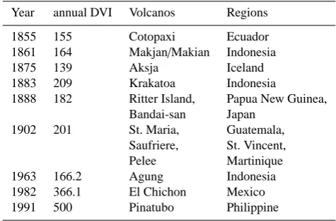
Table 2.Major volcanic eruptions from 1850 to 2000. DVI values

taken from the NCDC database.

Year annual DVI Volcanos Regions

1855 155 Cotopaxi Ecuador

1861 164 Makjan/Makian Indonesia

1875 139 Aksja Iceland

1883 209 Krakatoa Indonesia

1888 182 Ritter Island, Papua New Guinea,

Bandai-san Japan

1902 201 St. Maria, Guatemala,

Saufriere, St. Vincent,

Pelee Martinique

1963 166.2 Agung Indonesia

1982 366.1 El Chichon Mexico

1991 500 Pinatubo Philippine

be caused by some sudden but natural forcings, e.g. vol-canic eruptions (Mart´ınez et al., 2010). The eruptions are ac-companied by the injection of SO2and dust into the

strato-sphere. The increase of the dust and aerosol load in the stratosphere causes a reduction of the solar radiation in the lower atmosphere and leads to changes in the lower atmo-sphere circulation patterns during 2–4 yr after the eruptions (Robock, 2000). Table 2 shows major volcanic eruptions with the dust volcanic index (DVI) reaching more than 100 (from Mann et al., 2000 and NCDC database) from 1850 to 2000. The inhomogeneities that coincide with periods of strong eruptions (1855–1856, 1861–1862, 1875, 1883–1904, 1963– 1964, 1982–1984, and 1991–1994) could be of natural (vol-canic) origin, provided there were no records of instrumental changes for such epochs. In case some instrumental changes did take place during these periods, it would be difficult to make reasonable corrections only for the non-climatic part of these particular breaks.

2.4 Sea-surface temperature anomalies series

Monthly SST anomalies series (relative to the 1961–1990 pe-riod), obtained with HadISST2.0.0.0 (Rayner et al., 2012) in 2 grid points near the Portuguese coast during the period from 1899 to 2010, have been used as reference series to per-form relative homogeneity tests and calculate CRMSE val-ues. These series (comprised of a combination of 10 ensem-ble members) were extracted for the grid cells located be-tween 8–9◦_{W and 41–42}◦_{N in the case of the Porto nearest}

grid point and between 9–10◦_{W and 38–39}◦_{N for Lisbon.}

Table 3.Known dates of changes in thermometer heights (ht) and locations for the three Portuguese stations of Lisbon, Coimbra and Porto.

Station years Character of changes Correction

Lisbon 1864 Moved to a new building (distance is about 1 km) yes

Lat. 38◦

430

N 1918 Thermometer height change (+4.1 m) no

Long. 9◦₀₉0_{W 1920 Thermometer height change (−4.1 m) no}

Alt. 77 m 1929 Thermometer height change (+4.1 m) no

ht=1.6 m 1937 Thermometer height change (+0.7 m) no

1941 Thermometer height change (−22.2 m) yes

1977 Changes in the observation periodicity no

1980 Minor changes in the location (within the same garden) no

Coimbra 1922 Relocation of instrument park; installation of standard shelter yes Lat. 40◦

120

N 1933 Minor relocation yes

Long. 8◦

250

W 1950 Thermometer height change (from 1.15 m to 1.45 m) no

Alt. 141 m

ht=1.5 m

Porto Lat. 41◦

080

N

1916 Moved to new location; thermometer height change (from 10.3 m to 1.3 m above the ground)

yes

Long. 8◦₃₆0_W

Alt. 93 m

Sep 1920–Feb 1922 No measurements,

Probable change in instrument

no

ht=1.3 m 1947 Changes in the measurement times no

1984 Changes in the measurement times no

Table 4.Correlation coefficients between the temperature series from Porto and Lisbon (rL) and Coimbra (rC) calculated for the period

1910–1932 (±10 yr around the gap). Significances of the correlation coefficients (p) are smaller than 0.02 with only one exception: p=0.37 for correlation coefficients between Tminof Porto and Lisbon in June (m6). Regression coefficients (A, L, C) for regression models (Porto Tmin/max=A+L×Tmin/max(Lisbon)+C×Tmin/max(Coimbra)) are chosen using the best subset procedure with maximization of adj.R2parameter and calculated using data for the period 1910–1932 (±10 yr around the gap). (adj.R2_{×100) values show the percent of the variability of the} dependent variables (Porto Tminand Tmaxseries) that has been accounted for by the model under consideration.

Tmin Tmax

rL rC A L C adj.R2_{×100 rL rC A L C adj.R}2_×100

m1 0.81 0.82 −1.84 0.54 0.53 67.2 0.66 0.86 1.04 0 0.92 70.7

m2 0.90 0.91 −3.89 0.73 0.56 83.7 0.86 0.97 0.36 −0.2 1.09 94.5

m3 0.82 0.89 1.31 0 0.78 79 0.89 0.96 −2.72 0.15 0.88 92

m4 0.56 0.72 0.9 0 0.87 52.9 0.88 0.92 0.07 0.1 0.81 84.3

m5 0.75 0.72 −2.55 1 0 59.6 0.92 0.85 −3.85 0.67 0.34 91

m6 0.21 0.58 9.14 −0.22 0.61 31.6 0.87 0.96 1.67 −0.17 0.97 90.8

m7 0.57 0.75 1.4 0 0.91 58.9 0.92 0.95 −0.67 0.33 0.54 90.2

m8 0.51 0.66 4.79 0 0.66 41.9 0.82 0.93 −1.28 −0.1 0.95 80.8

m9 0.75 0.83 0.55 0 0.94 68.6 0.84 0.92 0.15 0.19 0.67 80.7

m10 0.52 0.58 3.65 0 0.66 30 0.90 0.91 −2 0.63 0.33 83.3

m11 0.74 0.83 −0.13 0 1 67.2 0.76 0.56 −1.85 0.76 0.2 57.1

m12 0.76 0.77 1.14 0 0.85 58.2 0.51 0.54 8.17 0.12 0.26 21.8

In the current analysis the SST series measured near Porto (mean of 10 ensemble members, later on “SST Porto”) have been used as reference series for Porto temperature series ho-mogenization, and SST series measured near Lisbon (mean of 10 ensemble members, later on “SST Lisbon”) have been used in the homogenization of Lisbon temperature series.

3 Porto (Serra do Pilar) temperature series

3.1 Data description and metadata

The original data set contains monthly averages of daily min-imum (Tmin) and maximum (Tmax) temperature and their

114 yr. Measurement errors are ±0.2◦_{C (valid for all}

ob-served temperature series presented here).

The meteorological station of Porto has been in regular operation since 1888 when it was put under the jurisdiction of the Observat´orio Meteorol´ogico da Princesa D. Am´elia, now IGUP, on the south part of the river Douro. In 1916 the station location was changed slightly and the thermometer was moved from the tower (10.3 m above the ground) to the ground level (1.3 m above the ground). The data set has a gap from September 1920 to February 1922; there is also a pos-sibility that the thermometer was replaced in March 1922. In 1947 and again in 1984/1985, changes in the observa-tion times were made. Table 3 shows known dates of pos-sible non-climatic breaks due to instrument changes (Pinhal, 2008).

Changes in the location of the instruments could result in sudden jumps of the measured parameter values. Tmin

and Tmaxcould respond differently to changes in position of

the respective thermometers, depending on the character of the changes in the instrument’s environment (Aguilar et al., 2003). Therefore, the variations of DTR could be more im-portant for the detection of the breaks; breaks could be weak in the Tminor Tmaxseries, but clearly seen in DTR series

(Wi-jngaard et al., 2003). The following parameters have been analysed (valid for all temperature series presented here):

1. minimum temperature (Tmin);

2. maximum temperature (Tmax);

3. temperature range (DTR =Tmax−Tmin);

4. monthly average temperature (Taver=(Tmax+Tmin)/2).

All series contain monthly and annual means; Tminand Tmax

are measured values, DTR and Taverare calculated values. To

perform relative homogeneity tests, the differences between standardized Tmin, Tmaxand Taverseries and standardized SST

Porto series were calculated.

3.1.1 Interpolation of the gap from September 1920 to February 1922

The gap in the data from September 1920 to February 1922 should be filled before the data are subjected to the homo-geneity analysis. It is possible to fill the gap using the simple linear interpolation for the absent one or two values for each of the monthly data series. On the other hand, it is possible to build a mathematical regression model for a more realistic in-terpolation, using data from nearby meteorological stations, namely, Coimbra and Lisbon data series. All 12 monthly se-ries of Tmin and Tmaxwere interpolated separately. The time

period used for the regression models is 10 yr before the gap (1910–1919) plus 10 yr after the gap (1923–1932).

First, the correlation coefficients (r) between temperature parameters measured in Porto and Coimbra and Lisbon were

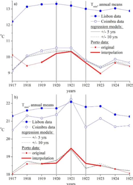
Figure 2.Variations of Tmin (a) and Tmax (b) measured in

Lis-bon, Coimbra and Porto-Serra do Pilar from 1917 to 1925 (annual means) and approximations by multiple regression models for time periods of±5 and±10 yr around the gap – annual sums. Grey ver-tical lines mark the period of absent data. The bold red lines show the accepted interpolation.

calculated (see Table 4). The significances (p) of the corre-lation coefficients are smaller than 0.02 with a single excep-tion. There are strong correlations (r=0.51...0.92) between the temperature variations in Porto and Lisbon and Coimbra for almost all months with only one exception – the corre-lation between Porto and Lisbon series of Tmin (June, m6): rL=0.21, p=0.37. Nevertheless, it is still possible to use the

data from Lisbon and Coimbra as regressors for Porto data in multiple regression models.

Multiple regression models for Porto Tmin and Tmax

se-ries were built using the Coimbra and Lisbon data as re-gressors. The models have been built using the “best subset” method, maximizing the adj.R2_{parameter. The regression}

co-efficients are shown in Table 4 alongside with (adj.R2_×100)

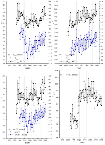
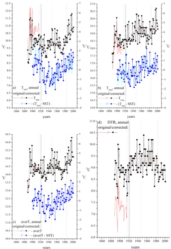
Figure 3.Porto: annual variations of Tmin(a), Tmax (b), Taver(c) and DTR (d); temperature series are shown in black, differences between temperature and SST Porto series are shown in blue. Grey vertical bands show dates of known instruments relocation (see Table 3).

data. Similar regression models have been calculated using a smaller time period:±5 yr around the gap (1915–1919 plus 1923–1927). However, the 5-yr-around-gap models give, in general, worse approximations for the real data than the 10-yr-around-gap models. Finally, the gap from September 1920 to February 1922 was interpolated using the 10-yr-around-gap multiple regression models for each parameter and for each month separately. Annual values of Tmin and Tmax for

1920–1922 have been calculated using both measured and

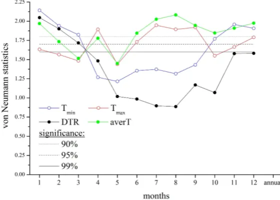
Figure 4.Porto: von Neumann ratio statistics for monthly series of Tmin, Tmax, DTR and Taver. Black straight lines show probability levels.

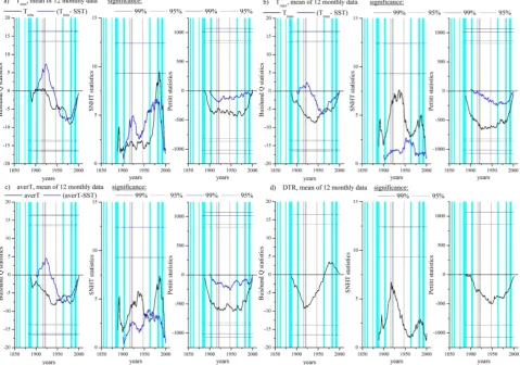
Figure 5.Porto: average of 12 monthly series of Buishand Q test (left panels), SNHT (middle panels) and Pettitt tests (right panels) statistics

of Tmin(a), Tmax(b), Taver(c) and DTR (d). Statistics of temperature series are shown in black, statistics of differences between temperature

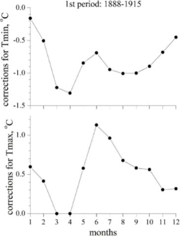
Figure 6.Porto: corrections (in◦

C) for Tmin(top panel) and Tmax (bottom panel) series for the period before the break, 1888–1915.

interpolation does not ignore the real variations of the tem-perature parameters that took place (according to the records from Lisbon and Coimbra) from September 1920 to February 1922. In particular, the interpolation using multiple regres-sion models allowed us to preserve the following features that were observed in monthly series variations (not shown):

– higher than estimated by the linear interpolations values

of Tmin during the periods of November to December

1920 and July to October 1921;

– lower than estimated by the linear interpolations values

of Tminin May 1921;

– higher than estimated by the linear interpolations values

of Tmax in December 1920, January 1921, and during

the period from March to December 1921;

– lower than estimated by the linear interpolations values

of Tmaxin October 1920 and in February and May 1921.

3.2 Homogenization 3.2.1 Visual analysis

Figure 3a–d show time variations of the annual series of Tmin, Tmax, Taver and DTR, respectively. The grey vertical lines

mark the dates of known changes in thermometer position. DTR variations (Fig. 3d) show at least one easily detectable break in 1916. This break corresponds to the most signifi-cant change in the instruments location: movement to a new

place and relocation of the instruments from the top of the tower to the ground level. The changes in the measurements times (in 1947 and 1984) and possible changes in the instru-ment park after the gap in 1922 could not be easily detected by the visual analysis. The break in 1916 has different ef-fects on the monthly Tmin and Tmaxvariations (not shown).

There are significant jumps in the monthly Tmin variations

clearly seen during warm months (from April to September). However, there are no jumps in the monthly Tmaxvariations

that could be easily detected by the visual analysis. This dif-ference could be explained by the different sensitivity of the

Tminand Tmaxto the change in location and in the instrument

height.

3.2.2 Homogeneity tests results

Figure 4 shows the von Neumann ratio for 12 monthly series of Tmin, Tmax, DTR and Taver. This test shows strong

inhomo-geneities in all four series and DTR in particular. As one can see, variations of the homogeneity of the data series strongly depend on the temperature parameter:

– Tmin – data series of warm months (from April to September) are more inhomogeneous than of cold ones;

– Tmax – data series of warm months (from April to

September) are less inhomogeneous than of cold ones with one exception – May;

– DTR – data series of two months only (January and

February) are apparently homogeneous;

– Taver– these data are more homogeneous than Tminand Tmax. They could be labelled as inhomogeneous with a

probability of 95 % only in March and May.

Figure 5a–d show test statistics (absolute and relative) for Buishand, SNHT and Pettitt test for Tmin, Tmax, Taver and

DTR, respectively. The average of 12 monthly statistics se-ries is plotted in these figures to emphasize the main fea-tures of each homogeneity test statistics and for better visu-alisation. From Fig. 5a–d it is possible to detect the strongest break in data homogeneity around 1916 – date of movement to a new location and change in the thermometers height. Also, for some months (not shown) there are breaks in the homogeneity around 1920s (gap and probable change of the thermometer), 1930s (unknown origin), 1947 (changes in the measurements time), 1963 (volcanic eruption), and 1984 (changes in the measurements time, which coincide with vol-canic eruptions).

Figure 7.Porto: original and corrected annual series of Tmin(a), Tmax(b), Taver(c) and DTR (d); temperature series are shown in black and red, differences between temperature and SST Porto series are shown in blue and cyan. Grey vertical bands show dates of known instruments relocation (see Table 3).

1984. This conclusion was confirmed later during the correc-tion procedure (Sect. 3.3.1) – correccorrec-tion of possible breaks in 1922 and 1947 makes the corrected series even more in-homogeneous.

3.2.3 Preliminary conclusions

Tmindata set shows inhomogeneities in 1916, near the 1920s,

1947, 1963 and 1984; Tmaxdata set showed inhomogeneities

in 1916, near the 1920s, 1930s, 1947, 1963 and, 1984; DTR data set showed strong inhomogeneity during the period 1916–1922 and, probably, a weak break in the 1940s; Taver

Figure 8.Porto: same as Fig. 4 but for the corrected series.

Figure 10.Porto: scatter plots of CRMSE before and after homogenization of 12 monthly and the annual series for Tmin(left) and Tmax (right). SST Porto anomalies data are used as reference series. Dots on or below the bisect indicate data sets with unchanged or improved (increased) homogeneity, while dots above the bisect indicate data sets with increased inhomogeneity.

1984; Tminduring warm months and Tmaxduring cold months

are more inhomogeneous than in other months. The inhomo-geneities that are not associated to known dates of instru-mental changes may be due to the internal climatic varia-tions caused, for example, by major volcanic erupvaria-tions. The most significant non-climatic break occurred in 1916 due to changes in the instruments location and height. This break requires correction. Other breaks detected by homogeneity tests have no statistically significant effect or could not be corrected due to the coincident influence of other (climatic) forces.

3.3 Correction for non-climatic breaks 3.3.1 Correction procedure

To correct the non-climatic breaks we used the procedure de-scribed in Sect. 2.2. The best corrections were obtained when

Tminand Tmaxdata sets were divided into two periods: 1888–

1915 and 1916–2001. For each month the means of tempera-ture parameters for certain time intervals (±5 yr for Tminand

±15 yr for Tmax) around 1916 were calculated. The data for

the 1888–1915 period were corrected using the correction values calculated as described above. All correction values are shown in Fig. 6. The corrections were applied to Tminand Tmaxdata sets. Afterwards, corrected values of DTR and Taver

were calculated. Results of the correction as well as original data are shown in Fig. 7a–d. Please note that due to the use of standardized values, the difference between temperature series and SST anomalies presented in Fig. 7 (and similar for

other stations) show differences between corrected and orig-inal series even for non-corrected periods – the series means and standard deviations that are used in the standardizing procedure change after correction.

3.3.2 Homogeneity of the corrected series

All four corrected data sets were subjected to the same ho-mogeneity tests as the original data. The results of these tests for Tmin, Tmax, Taverand DTR are shown in Figs. 8 and 9a–

d (similarly to Figs. 4–5). As one can see from the com-parison of similar statistics for the original (Figs. 4–5) and corrected (Figs. 8–9) data, the latter data sets are less inho-mogeneous but still contain inhomogeneities coinciding with the volcanic eruptions that occurred in the end of the 19th and 20th centuries. Some absolute tests for some months (not shown) still show breaks of homogeneity in a period lasting from 1922 to 1947, although there is no consistency between the three homogeneity tests (Buishand and Pettitt tests and SNHT) in relation to the dates of the breaks. The relative ho-mogeneity tests showed an almost total absence of the breaks around dates of known instrument changes. Therefore, the corrections for these breaks were not necessary. The homo-geneity level given by the von Neumann ratio of the corrected data series (Fig. 8) still depends on the temperature parame-ter; among all parameters Tminis the least homogeneous. One

of the possible reasons for the remaining inhomogeneities in the Tmin data series is the volcanic effect. Figure 10 shows

Figure 11.Lisbon: annual variations of Tmin(a), Tmax(b), Taver(c) and DTR (d); temperature series are shown in black, differences between temperature and SST Lisbon series are shown in blue. Grey vertical bands show dates of known instruments relocation (see Table 3).

As one can see, the inhomogeneity level of both Tmin (left

panel) and Tmax(right panel) decreases or stays unchanged

for all monthly series.

Breaks detected in the corrected data sets by the different homogeneity tests are rarely coincident, except for the end of the 20th century (an epoch of El Chichon and Pinatubo erup-tions – see Table 2). Sometimes the tests still show breaks of homogeneity during different periods but there is no con-sistency between the three homogeneity tests (Buishand and

Pettitt tests and SNHT) in the dates of the breaks. In our opin-ion, these inhomogeneities are caused by the application of the correction values which are already smoothed by a 3-months adjacent average to maintain the annual cycle (see Sect. 2.2) and we believe that in these cases additional cor-rections are not necessary. Thus, we consider the data sets of Tminand Tmaxcorrected by the procedure described in the

Figure 12.Lisbon: von Neumann ratio statistics for monthly series of Tmin, Tmax, DTR and Taver. Black straight lines show probability levels.

Figure 13.Lisbon: average of 12 monthly series of Buishand Q test (left panels), SNHT (middle panels) and Pettitt tests (right panels)

Figure 14.Lisbon: corrections (in◦_{C) for T}

min(top panels) and Tmax(bottom panels) series for two periods between the breaks 1856–1863 (left panels) and 1864–1940 (right panels).

4 Lisbon IGIDL temperature series

4.1 Data description and metadata

The original data sets contain monthly averages of daily min-imum (Tmin) and maximum (Tmax) temperature and their

an-nual means measured at Instituto Geof´ısico do Infante D. Lu´ıs (IGIDL), Lisbon from 1856 to 2008. The data sets length is 153 yr.

The meteorological station of Lisbon/Geof´ısico has been in regular operation since October 1854. During the first ten years the thermometers were positioned in the terrace of the Observatory Tower of the old Escola Polit´ecnica, located in the Jardim Botˆanico. This three-storied tower was built in 1854, thus leading to the foundation of the Infante D. Luiz Observatory (now IGIDL). This building proved inadequate for systematic observations and a new 4-storied tower was inaugurated in October 1863 in the main central edifice of Escola Polit´ecnica, with the thermometers being reinstalled in the new terrace. This building still houses the IGIDL to-day and some of its meteorological instruments, but the park of instruments containing the thermometers (the Stephenson shelter), initially installed on the platform of the new ob-servatory tower, was transferred to the grounds in Jardim Botˆanico in 1941 (the distance between the two locations is about 120 m). In 1979 the Jardim Botˆanico’s instrumental park location was slightly changed. Additionally, in January 1977 changes in the times of observation have been made (Carvalho, 2001). Table 3 summarizes the information about possible non-climatic breaks that could appear in the Lis-bon/Geof´ısico temperature series.

To perform relative homogeneity tests, the differences be-tween standardized Tmin, Tmaxand Taverseries and

standard-ized SST Lisbon series were calculated.

4.2 Homogenization 4.2.1 Visual analysis

Figure 11a–d show the time variations of the annual series of Tmin, Tmax, Taverand DTR, respectively. As one can see,

DTR variations (Fig. 11d) show two easily visible breaks in 1863/1864 and 1940/1941. These breaks correspond to the two most significant changes in the instruments location: movement to a new place in 1864 and relocation of the in-struments from the top of the tower to the ground level in 1941. At first sight, it seems that the minor changes in the thermometers height that took place from 1917 to 1937 and minor changes in the instruments location in 1979 were too small to have a significant influence on the data homogeneity. These two breaks have different influences on the Tminand Tmax variations (see Fig. 11a and b). As one can see,

dur-ing the first break (1864) there are significant jumps both in

Tmin and Tmax. However, during the second break in 1941

there is a significant jump in Tmax but a very small one (if

any) in Tmin. On the contrary, the difference between Tmin

and SST (Fig. 11a, blue line) has a significant jump in 1941, whereas the difference between Tmaxand SST (Fig. 11a, blue

Figure 15.Lisbon: original and corrected annual series of Tmin(a), Tmax(b), Taver(c) and DTR (d); temperature series are shown in black and red, differences between temperature and SST Lisbon series are shown in blue and cyan. Grey vertical bands show dates of known instruments relocation (see Table 3).

4.2.2 Homogeneity tests results

The von Neumann test statistics for the 12 monthly series of

Tmin, Tmax, Taverand DTR are shown in Fig. 12. The

vari-ations of the homogeneity of monthly data series (given by the von Neumann ratio) strongly depend on the temperature parameter:

– Tmin– data series of warm months are more

inhomoge-neous than of cold ones;

– Tmax – all months show strong inhomogeneity except August (m8);

Figure 16.Lisbon: same as Fig. 12 but for the corrected series.

Figure 18.Lisbon: scatter plots of CRMSE before and after homogenization of 12 monthly and the annual series for Tmin(left) and Tmax (right). SST Lisbon anomalies data are used as reference series. Dots on or below the bisect indicate data sets with unchanged or improved (increased) homogeneity, while dots above the bisect indicate data sets with increased inhomogeneity.

– DTR – data series of warm months are more

inhomoge-neous than of cold ones.

The average of 12 monthly test statistics series (absolute and relative) for Buishand, SNHT and Pettitt test for Tmin, Tmax, Taverand DTR for annual series are shown in Fig. 13a–d,

re-spectively. The grey vertical lines mark the dates of known changes in thermometer position. As one can see, some of these dates (namely, 1864 and the period from 1916 to 1941) coincide with significant breaks depicted by the maxima (or minima) of the curves. It should be mentioned that for Tmin

the coincidences between the known instrumental changes dates and break years detected by the absolute tests are rare, whereas for Tmax, DTR and Taverthese coincidences are very

frequent. Also, there are two periods of possible break years detected by the homogeneity tests that do not coincide with known dates of instrument changes: one is at the end of the 19th century/beginning of 20th century (approx. from (1880) 1890 to 1900) and the second is at the end of the 20th cen-tury (approx. from 1970 to 1990). Relative homogeneity tests (blue lines) of Tmin show significant breaks around 1937

(small changes in the thermometer height) and homogeneity tests of Tmaxshow significant breaks around 1941.

4.2.3 Preliminary conclusions

Tmin data sets show inhomogeneities in the 1860s, near

1970s–1980s and, possibly, near 1880s–1890s; Tmaxis more

sensitive than Tminto the changes of the thermometer height

that took place in 1864 and from 1916 to 1941. Tmax data

sets show strong inhomogeneity during this period. There are also some inhomogeneities near 1880s–1890s and 1970s–

1980s; DTR and Taver show the same three periods of

in-homogeneity: near 1880s–1890s, 1910s–1940s and 1970s– 1980s. Temperature series of warm months contain more inhomogeneities than those of cold months. The inhomo-geneities that are not associated to known dates of instrumen-tal changes could appear due to the internal climatic varia-tions caused by, e.g. major volcanic erupvaria-tions. The most sig-nificant non-climatic breaks have occurred in 1864 and 1941 due to changes in the instruments location (1864) and height (1941). These breaks have to be corrected.

Small changes in the thermometer height took place from 1917 to 1936 and the short periods between the changes do not allow us to estimate statistically significant corrections. The dislocation of the station in 1979 does not significantly (with significance 95 % or more) affect the homogeneity of the data – the means of the temperature parameters for 1941– 1978 and 1979–2008 are the same within the instrumental and statistical errors.

4.3 Correction for non-climatic breaks 4.3.1 Correction procedure

The Tminand Tmaxdata sets were divided into three periods:

1856–1863, 1864–1940, and 1941–2008. We started from the most recent break – 1940/1941. For each month the means of temperature parameters for certain time intervals (±20 yr for Tmin and±45 yr for Tmax) around 1941 were calculated.

The second break (1863/1864) was corrected using means calculated for time intervals 1864±8 yr both for Tmin and Tmax. All correction values are shown in Fig. 14. As one can

Figure 19.Coimbra: annual variations of Tmin (a), Tmax (b), Taver (c) and DTR (d); Coimbra temperature series (black) and differences between Coimbra and Porto (blue) and Lisbon (green) temperature series. Grey vertical bands show dates of known instruments relocation (see Table 3).

Tmaxare non-zero for all months whereas the corrections for Tminare equal to zero for months from March to June (m3–

m6). Results of the correction as well as of the original data are shown in Fig. 15a–d for annual series.

4.3.2 Homogeneity of the corrected series

All four corrected data sets were subjected to the same ho-mogeneity tests as the original data. The results of these tests

of Tmin, Tmax, Taverand DTR are shown in Figs. 16 and 17a–d

Figure 20.Coimbra: von Neumann ratio statistics for monthly series of Tmin, Tmax, DTR and Taver. Black straight lines show probability levels.

Figure 21.Coimbra: average of 12 monthly series of Buishand Q test (left panels), SNHT (middle panels) and Pettitt tests (right panels)

Figure 22.Coimbra: corrections (in◦

C) for Tmin(top panels) and Tmax(bottom panels) series for two periods between the breaks; 1865–1921 (left panels) and 1922–1932 (right panels).

almost in all months. The possible reason for the remain-ing inhomogeneities in the Tmin series is the volcanic effect

clearly seen in Fig. 17a–d.

Figure 18 shows CRMSEs of corrected series (SST Lis-bon are used as reference series) plotted versus correspond-ing CRMSEs of the original series. As one can see, the inho-mogeneity level of Tmin(left panel) slightly decreases – dots

are lower than the bisect; on the contrary, the inhomogeneity level of Tmax(right panel) stays almost the same for 10 out of

12 monthly series but CRMSE of two monthly series slightly increases.

Sometimes the tests still show breaks of homogeneity in the period from 1917 to 1936 but there is no consistency be-tween the three homogeneity tests (Buishand and Pettitt tests and SNHT) in the dates of the breaks. In our opinion, these inhomogeneities are caused again by the application of the smoothed correction values and we believe that in these cases additional corrections are not necessary. Thus, we consider the data sets of Tminand Tmaxcorrected by the procedure

de-scribed in the paper as free of non-climatic changes with a significance of at least 95 %.

5 Coimbra IGUC temperature series

5.1 Data description and metadata

The original data set contains monthly averages of daily min-imum (Tmin) and maximum (Tmax) temperature and their

an-nual means measured at Instituto Geof´ısico da Universidade de Coimbra (IGUC), Coimbra from 1865 to 2005. The data set length is 141 yr.

Accordingly to IGUC logbooks, during the entire period (1865–2005) the meteorological station remained in the same

location – the park of IGUC. However, the park of instru-ments has undergone some changes in position and envi-ronment described in Table 3. There were two more or less significant changes in the instruments location in 1922 and 1933; besides that, the standard (Stephenson’s) shelter was installed in 1922 and in 1950 the thermometer height in-creased slightly (from 1.15 m to 1.45 m). Since Coimbra is not a coastal station, the already corrected temperature series for Porto and Lisbon were used as reference series; the diff er-ences between Tmin, Tmaxand Taverseries and corresponding

series for Porto and Lisbon were calculated to perform rela-tive homogeneity tests.

5.2 Homogenization 5.2.1 Visual analysis

Figure 19a–d show time variations of the annual series of

Tmin, Tmax, Taverand DTR, respectively. The DTR variations

show easily a visible break in 1921/1922 (relocation of the instruments and installation of the shelter) coinciding with a significant jump in Tmin(Fig. 19a), but not in Tmax(Fig. 19b).

Another break probably appears in 1949/1950 (changes in thermometer height); it can be seen both in Tmin and Tmax

data. This break is however absent in DTR data (probably, due to almost equal shifts in Tminand Tmax). There is also a

small break in 1932/1933 (small relocation).

5.2.2 Homogeneity tests results

Figure 23.Coimbra: original and corrected annual series of Tmin(a), Tmax(b), Taver(c) and DTR (d); Coimbra temperature series (red and black) and differences between Coimbra and Porto (cyan and blue) and Lisbon (dark green and green) temperature series. Grey vertical bands show dates of known instruments relocation (see Table 3).

– Tmin – data for months from February to June (m2 to

m6) are more inhomogeneous than others;

– Tmax– all months show strong inhomogeneity;

– DTR – data for months of the second half of the year

are more inhomogeneous than others;

– Taver– data from February to June and October (from

Figure 24.Coimbra: same as Fig. 20 but for the corrected series.

Figure 26.Coimbra: scatter plots of CRMSE before and after homogenization of 12 monthly and the annual series for Tmin (left) and Tmax(right). Corrected Porto (top panels) and Lisbon (bottom panels) temperature series are used as reference series. Dots on or below the bisect indicate data sets with unchanged or improved (increased) homogeneity, while dots above the bisect indicate data sets with increased inhomogeneity.

series of Tmin, Tmax, Taverand DTR are shown in Fig. 21a–

d, respectively. It should be mentioned that SNHT statistics, both for annual and monthly Tmax, show an unexpected

be-haviour: despite the absence of any jumps in the temperature data, the SNHT statistic shows strong inhomogeneities at the end of the data set (2002–2005). These inhomogeneities do not correlate with inhomogeneities detected on the same data by other tests. This unexpected behaviour could be explained by the known tendency of the SNHT to generate false alarm results close to the start and the end of data sets (Wang, et al., 2007). Therefore, to disambiguate the interpretation, Fig. 21b does not show SNHT statistics for Tmaxduring 2002–2005 yr.

The analysis of the homogeneity tests statistics provides the most probable time periods of the breaks in the data ho-mogeneity: around 1885–1890, around 1905, around 1916, around 1920, around 1930–1936, in the 1940s, 1960s and 1980s. Many inhomogeneities, which are detected by the tests but could not be associated with known instrumental changes, correspond to volcanic effects.

The comparison between homogeneity test statistics of Coimbra and Lisbon data shows more or less a similar character of the annual inhomogeneities variations for both places. These similarities arise from the relative proximity of Lisbon and Coimbra and likeliness in the character of their climatic variation as well as from the volcanic origin of a number of inhomogeneities of the data.

5.2.3 Preliminary conclusions

Tmaxdata showed more inhomogeneities than other

tempera-ture parameters; Tmindata sets showed inhomogeneities near

1880s, 1900s, 1920s, 1960s and 1980–1990s; DTR and Taver

showed strong inhomogeneities around 1885–1890, around 1905, around 1916, 1922, around 1930–1936, around 1941, in the 1960s and 1980s; and Tmin and Taver data had more

inhomogeneities during warm months. The inhomogeneity levels of Tmax and DTR data were more or less constant

throughout the year. The most significant non-climatic break occurred in 1922 due to changes in the instruments loca-tion. This break is clearly seen in relative homogeneity tests statistics both for Tmin and Tmax. Another break was

asso-ciated with the small relocation of the instruments park in 1933. This break is seen only in relative homogeneity tests statistics for Tmax. These two breaks required correction. The

change in the thermometer height in 1950 showed no signif-icant (significance 95 % or more) effect on the homogeneity of the temperature data.

5.3 Correction for non-climatic breaks 5.3.1 Correction procedure

To correct the non-climatic breaks, Tmin and Tmax data sets

were divided into three periods: 1865–1921, 1922–1932, and 1933–2004. We started from the most recent break – 1932/1933. This break was corrected only in Tmaxseries. For

around 1933 were calculated. The second break (1921/1922) was corrected both in Tmaxand Tminseries using intervals of

±10 yr for Tmaxand±40 yr for Tmin. All correction values are

shown in Fig. 22. Results of the corrections as well as origi-nal data are shown in Fig. 23a–d for annual series.

5.3.2 Homogeneity of the corrected series

All four corrected data sets were subjected to the same homo-geneity tests as the original data. The results of these tests for

Tmin, Tmax, Taverand DTR are shown in Figs. 24 and 25a–d

(similarly to Fig. 21). As one can see from the comparison of homogeneity test statistics of original (Figs. 20–21) and cor-rected (Figs. 24–25) series, the corcor-rected data sets are less inhomogeneous. The statistics of the relative homogeneity tests show much less inhomogeneities in the corrected series than statistics of absolute homogeneity tests. The corrected series still contain inhomogeneities caused (probably) by the volcanic eruptions. It can be seen that, as a whole, the annual variations of the corrected data series homogeneity given by the von Neumann ratio still depends on the temperature pa-rameter; Tminis the less homogeneous among all parameters.

Despite the fact that annual series still contain non-climatic inhomogeneities, monthly series, in most cases, are free of them. For a couple of months homogeneity tests still show breaks in homogeneity in the period from 1922 to 1933, but there is no consistency between the three homogeneity tests (Buishand and Pettitt tests and SNHT) in the dates of breaks. Figure 26 shows CRMSEs of corrected series (cor-rected Porto and Lisbon temperature series are used as ref-erence series), plotted versus CRMSEs of the original series. As one can see, the inhomogeneity level of Tmin (left

pan-els) decreases slightly – dots are close to the bisect, whereas on the contrary the inhomogeneity level of Tmax (right

pan-els) significantly decreases for all monthly series when com-pared to Lisbon temperature series (low panel) and for 10 monthly series when compared to Porto temperature series (top panels). These homogeneity tests allow one to consider the corrected series of Tminand Tmaxas free of non-climatic

changes with a significance of at least 95 %.

6 Conclusions

Homogeneity tests show the presence of strong non-climatic breaks in all temperature series. Most of the detected breaks were corrected and the homogeneity tests of the corrected series show no significant (significance 95 % or more) breaks around dates of instrumental changes.

6.1 Porto

One strong non-climatic break was detected in the tem-perature series of Porto Serra do Pilar, IGUP. This break was caused by the changes in the instruments location and

height (1916). This break did not coincide with known vol-canic eruptions of significant strength and required correc-tion. Other breaks detected by the homogeneity tests either had low levels of significance (lower than 95 %) or coin-cided with (probably caused by) strong volcanic eruptions. Such was the case of the possible non-climatic break in 1984, which could not be corrected due to the aforementioned co-incidence. The break that took place in 1916 was corrected.

6.2 Lisbon

Two strong non-climatic breaks were detected in the tem-perature series of Lisbon, IGIDL. These breaks were caused by the changes in the instruments location (1864) and height (1941). These breaks were corrected. Other breaks detected by the homogeneity tests had low levels of significance (lower than 95 %).

6.3 Coimbra

Two strong non-climatic breaks were detected in the temper-ature series of Coimbra, IGUC. These breaks were caused by the changes in the instruments location (1922 and 1933). These breaks were corrected.

Acknowledgements. The authoresses would like to thank

IGIDL, IGUC and IGUP for supplying the temperature data up to 1940. Also Instituto de Meteorologia, I.P. for supplying the post 1940 data and the UK Meteorological Office Hadley Centre for giv-ing us the HadISST2.0.0.0 data.

We would like to thank personally Alexandra Pais, Jo˜ao Fernandes and Ivo Alves from Centro de Geof´ısica da Universidade de Coim-bra and Maria Jos´e Neves Chorro currently from Universidade de Aveiro for supplying the data and for their helpful scientific discus-sions. We are indebted to Leopold Haimberger of the University of Vienna for reading the first draft and suggesting the use of reference series.

Anna Morozova was supported by a Post-Doc FCT scholarship (ref.: SFRH/BPD/74812/2010). This work was developed in the context of FP7 project ERA-CLIM (Grant Agreement Nr. 265229).

Edited by: G. K¨onig-Langlo

References

Aguilar, E., Auer, I., Brunet, M., Peterson, T. C., and Wieringa, J.: Guidance on metadata and homogenization, WMO-TD No. M.1186, (WCDMP-No. 53), 1–55, 2003.

Alexandersson, H. and Moberg, A: Homogenization of swedish temperature data. Part I: Homogeneity test for linear trends, Int. J. Climatol., 17, 25–34, 1997.

Buishand, T. A.: The analysis of homogeneity of long-term rainfall records in The Netherlands, R. Neth. Meteorol. Inst. (K.N.M.I.), De Bilt, Sci. Rep. No. 81-7, 77 pp., 1981.

Carvalho, A. C. F. J.: Tendˆencias da m´edia e variabilidade clim´atica em algumas estac¸˜oes meteorol´ogicas de Portugal continental, Li-cenciatura Dissertation, Faculdade de Ciˆencias da Universidade de Lisboa, 59 pp., 2001.

Costa, A. C. and Soares, A.: Homogenization of climate data: re-view and new perspectives using geostatistics, Math. Geosci., 41, 291–305, 2009.

Gleckler, P. J., Taylor, K. E., and Doutriaux, C.: Performance metrics for climate models, J. Geophys. Res., 113, D06104, doi:10.1029/2007JD008972, 2008.

Khaliq, M. N. and Ouarda, T. B. M. J.: On the critical values of the standard normal homogeneity test (SNHT), Int. J. Climatol., 27, 681–687, 2007.

Klein Tank, A. M. G.: Algorithm Theoretical Basis Document (ATBD), European Climate Assessment & Dataset (ECA&D) project document, KNMI, 38 pp., 2007.

Mann, M. E., Gille, E. P., Bradley, R. S., Hughes, M. K., Over-peck, J. T., Keimig, F. T., and Gross, W. S.: Global Temperature Patterns in Past Centuries: An Interactive Presentation, Earth In-teract., 4, 1–29, 2000.

Mart´ınez, M. D., Serra, C., Burgue˜no, A., and Lana, X.: Time trends of daily maximum and minimum temperatures in Catalonia (ne Spain) for the period 1975–2004, Int. J. Climatol., 30, 267–290, doi:10.1002/joc.1884, 2010.

NCDC database: http://www.ncdc.noaa.gov/paleo/ei/ei data/ volcanic.dat, last access: 19 September 2011.

Peterson, T. C., Easterling, D. R., Karl, T. R., Groisman, P., Nicholls, N., Plummer, N., Torok, S., Auer, I., Boehm, R., Gul-lett, D., Vincent, L., Heino, R., Tuomenvirta, H., Mestre, O., Szentimrey, T., Salinger, J., Førland, E. J., Hanssen-Bauer, I., Alexandersson, H., Jones, P., and Parker, D.: Homogeneity ad-justments of in situ atmospheric climate data: a review, Int. J. Climatol., 18, 1493–1517, 1998.

Pettitt, A. N.: A Non-Parametric Approach to the Change-Point Problem, Appl. Stat.-J. Roy. St. C., 28, 126–135, 1979.

Pinhal, E. O. S.: Variabilidade interdecadal da temperatura, press˜ao e precipitac¸˜ao do Observat´orio da Serra do Pilar, Teses de mestrado, Universidade de Lisboa, Lisboa, 96 pp., 2008. Rayner, N. A., Kennedy, J. J., Titchner, H. A., Saunby, M., and

Saunders, R. W.: The development of the new Hadley Centre Sea Ice and Sea-surface temperature dataset, HadISST2, to ex-plore uncertainty in boundary forcing for reanalysis, Poster Pre-sentation, 4th World Climate Research Programme International Conference on Reanalyses, Silver Spring, Maryland, USA, 7–11 May 2012.

Robock, A.: Volcanic eruptions and climate, Rev. Geophys., 38, 191–220, 2000.

Solow, A.: Testing for climatic change: an application of the two-phase regression model, J. Clim. Appl. Meteorol., 26, 1401– 1405, 1987.

Taylor, K. E.: Summarizing multiple aspects of model performance in a single diagram, J. Geophys. Res., 106, 7183–7192, 2001. Venema, V. K. C., Mestre, O., Aguilar, E., Auer, I., Guijarro, J.

A., Domonkos, P., Vertacnik, G., Szentimrey, T., Stepanek, P., Zahradnicek, P., Viarre, J., M¨uller-Westermeier, G., Lakatos, M., Williams, C. N., Menne, M. J., Lindau, R., Rasol, D., Rustemeier, E., Kolokythas, K., Marinova, T., Andresen, L., Acquaotta, F., Fratianni, S., Cheval, S., Klancar, M., Brunetti, M., Gruber, C., Prohom Duran, M., Likso, T., Esteban, P., and Brandsma, T.: Benchmarking homogenization algorithms for monthly data, Clim. Past, 8, 89–115, doi:10.5194/cp-8-89-2012, 2012. von Neumann, J.: Distribution of the Ratio of the Mean Square

Suc-cessive Difference to the Variance, Ann. Math. Stat., 12, 367– 395, 1941.

Wang, X. L., Wen, Q. H., and Wu, Y.: Penalized Maximal t Test for Detecting Undocumented Mean Change in Climate Data Series, J. Appl. Meteorol. Clim., 46, 916–931, 2007.