https://doi.org/10.5194/gmd-11-2541-2018 © Author(s) 2018. This work is distributed under the Creative Commons Attribution 4.0 License.
Geodynamic diagnostics, scientific visualisation and StagLab 3.0
Fabio Crameri
Centre for Earth Evolution and Dynamics (CEED), University of Oslo, P.O. Box 1028 Blindern, 0315 Oslo, Norway Correspondence:Fabio Crameri ([email protected])
Received: 31 December 2017 – Discussion started: 20 February 2018 Revised: 24 May 2018 – Accepted: 7 June 2018 – Published: 29 June 2018
Abstract. Today’s geodynamic models can, often do and sometimes have to become very complex. Their underlying, increasingly elaborate numerical codes produce a growing amount of raw data. Post-processing such data is therefore becoming more and more important, but also more challeng-ing and time-consumchalleng-ing. In addition, visualischalleng-ing processed data and results has, in times of coloured figures and a wealth of half-scientific software, become one of the weakest pillars of science, widely mistreated and ignored. Efficient and au-tomated geodynamic diagnostics and sensible scientific vi-sualisation preventing common pitfalls is thus more impor-tant than ever. Here, a collection of numerous diagnostics for plate tectonics and mantle dynamics is provided and a case for truly scientific visualisation is made. Amongst other diag-nostics are a most accurate and robust plate-boundary identi-fication, slab-polarity recognition, plate-bending derivation, surface-topography component splitting and mantle-plume detection. Thanks to powerful image processing tools and other elaborate algorithms, these and many other insight-ful diagnostics are conveniently derived from only a subset of the most basic parameter fields. A brand new set of sci-entific quality, perceptually uniform colour maps including
devon,davos,osloandbrocis introduced and made freely available (http://www.fabiocrameri.ch/colourmaps, last ac-cess: 25 June 2018). These novel colour maps bring a signif-icant advantage over misleading, non-scientific colour maps likerainbow, which is shown to introduce a visual error to the underlying data of up to 7.5 %. Finally, STAGLAB(http: //www.fabiocrameri.ch/StagLab, last access: 25 June 2018) is introduced, a software package that incorporates the whole suite of automated geodynamic diagnostics and, on top of that, applies state-of-the-art scientific visualisation to pro-duce publication-ready figures and movies, all in the blink of an eye and all fully reproducible. STAGLAB, a simple, flexible, efficient and reliable tool made freely available to
everyone, is written in MATLAB and adjustable for use with geodynamic mantle convection codes.
1 Overview
The first basic numerical geodynamic models were devel-oped in the early 1970s (e.g. Minear and Toksöz, 1970; Tor-rance and Turcotte, 1971). Since then they have become more powerful and often more complex (see e.g. King, 2001; Gerya, 2011; Lowman, 2011; Coltice et al., 2017). Indeed, dynamically self-consistent geodynamic models used to re-produce the first-order characteristics of the complex plate– mantle system, like mobile surface plates, single-sided sub-duction and mantle plumes, that need a certain complexity (e.g. Crameri and Tackley, 2015). However, this complex-ity often inhibits a simple understanding of the full inter-play between all individual physical aspects of these models: the models become too complicated to be easily explained or even fully understood. In addition, the more elaborate numerical codes powering these models (e.g. Zhong et al., 2000; Gerya and Yuen, 2007; Moresi et al., 2007; Tackley, 2008; Davies et al., 2011; Thieulot, 2014; Kaus et al., 2016; Heister et al., 2017) and the still increasing computational power available for their execution produce more and more raw data. The resulting amount of data to be processed easily exceeds the capability of a human scientist. Today, efficient, automated and intelligent geodynamic diagnostics are thus more important than ever to keep up with the advances made in numerical models.
of models (e.g. high-resolution and 3-D geometry) and new and improved visualisation techniques (e.g. coloured figures and movies). Worrisome visualisation pitfalls arise that make figures confusing, unreadable or even misleading and hence unscientific. Therainbowcolour map strongly deteriorates, for example, the underlying scientific data (Pizer and Zim-merman, 1983; Ware, 1988; Tufte, 1997) due to the inhomo-geneous colour sensitivity of the human retina (Thomson and Wright, 1947). On top of that, it is confusing to people with some of the most common colour-vision deficiencies. Even though all this has been known for awhile (see Rogowitz and Treinish, 1996, 1998; Light and Bartlein, 2004; Borland and Ii, 2007, and #endrainbow), therainbowcolour map is still commonly used by scientists and commonly accepted by sci-entific journals. In addition to the current need for more ad-vanced geodynamic diagnostics, it is thus clear that, today, efficient scientific quality visualisation has also become more important than ever.
Nevertheless, there is currently no tool available to per-form key geodynamic diagnostics and scientific visualisation efficiently and reliably. STAGLAB(http://www.fabiocrameri. ch/StagLab, last access: 25 June 2018) is the post-processing and visualisation software that aims to fill this gap and ful-fil all the necessities mentioned above. Previous versions of STAGLAB(Crameri, 2013, 2017a) were designed to specif-ically handle the raw data produced by the finite-difference, finite-volume multi-grid mantle convection code StagYY (Tackley, 2008). STAGLAB 3.0 (Crameri, 2017b), however, offers potential compatibility with other geodynamic codes as well and has, for example, already been tested successfully with output from the finite-element code Fluidity (Davies et al., 2011).
In the following, I will present key geodynamic diagnos-tics and how to automate them, discuss scientific and non-scientific colour schemes and visualisation approaches, and introduce STAGLAB, the all-in-one software package that makes powerful geodynamic diagnostics and state-of-the-art scientific visualisation easily accessible to everyone.
2 Geodynamic diagnostics
In science, it is desirable to rely on quantitative measures rather than on visual impression, also for reasons outlined in Sect. 3. Here, I list a variety of key diagnostics for the dynam-ics of the plate–mantle system that all can be automatised and applied to digital data. While some of these diagnostics are already well known, others are significantly improved or newly introduced here. The geodynamic diagnostics covered here are listed in Table 2 and explained in detail below and can be predominantly applied to 2-D data or vertical slices of Cartesian 3-D data. All of the diagnostics are tested and implemented in the software STAGLAB3.0 (see Sect. 4).
2.1 Generic flow diagnostics
A suite of generic flow diagnostics is often calculated and exported to file directly by fluid-dynamics codes (see e.g. Zhong et al., 1998; Tackley, 2000). These include, for exam-ple, root mean square (RMS) flow velocity, the Nusselt num-ber, which is the ratio of the total heat flux across a fluid layer to its conductive value (Chandrasekhar, 1961), heat flow and mean temperature. These are often either given as a func-tion of depth or as depth-average values. Other generic flow diagnostics like plateness and mobility, both characterising the surface boundary layer of mantle convection, are men-tioned below in more detail in addition to a list of different approaches to derive residual mantle temperatures.
2.1.1 Plateness
One of the key characteristics of ocean-plate tectonics is wide, almost rigid plate interiors bounded by localised, weak plate boundaries (Crameri et al., 2018). Plateness is a mea-sure of how localised the surface deformation is and thus for how well a surface represents ocean-plate tectonics (Wein-stein and Olson, 1992; Tackley, 2000). Plateness is derived from the second invariant of the strain rate on anxy plane spanning the surface
˙ εsurf=
q ˙ ε2
xx+ ˙εyy2 +2ε˙2xy, (1)
from which the total integrated ε˙surf and the surface-area fraction f80, in which the highest 80 % of that deforma-tion occurs, can be calculated (Tackley, 2000). For perfect plates, f80 would be zero, with deformation only taking place within infinitely narrow zones, while for uniformly dis-tributed plates,f80 would be 0.8. A non-dimensional plate-ness parameter,P, is finally derived by
P =1−f80 fc
, (2)
wherefcis the characteristic surface-area fraction for a flow with given vigour and heating mode, and is, for example,
fc=0.6 for internally heated convection with a Rayleigh number ofRaH=106(Tackley, 2000).
2.1.2 Mobility
Another key characteristic of ocean-plate tectonics is the mo-tion of the surface plate. Mobility is a measure of this momo-tion across a specified surface. It is simply defined by
M= vrms,surf vrms,global
, (3)
Table 1.Regional topographic characteristics.
Geometric characteristic Abbreviation Measurement methoda,b,c
Viscous fore-bulge FB FB=FB0−z2
Subduction trench TR TR=TR0
Island arc IA IA=IA0−z4
Back-arc depression depth BAD BAD=BAD0−z4 Back-arc depression extent BADextent BADextent=xTR−x3 Back-arc depression area BADarea BADarea=Rxx4
3z3−z(x)dx ax
1=0,x2=400 km,x3=x(z=z3)andx4=xTR.bz1=0 kmis the sea level,
z2=zmin(x > xFB),z4=zmean(x < x2)andz3=z4−2(zmax−zmin)forx < x2.cSee graphical representation in Fig. 2.
2.1.3 Residual mantle temperature
Extracting the residual temperature in a given domain is of-ten very insightful, as geodynamic flows are ofof-ten strongly temperature dependent and hence driven by the temperature anomalies. The residual mantle temperature can be defined in different ways. Most commonly, residual mantle tempera-ture is defined as the temperatempera-ture anomaly after normalising the temperature at each depth to the corresponding global horizontal mean (e.g. Labrosse, 2002). This definition is, however, less useful to distinguish local anomalies in global wide-aspect-ratio models. To distinguish a local anomaly, the field has to be normed to a regional instead of a global mean. Therefore, I outline here different ways of defining a residual mantle temperature.
1. Horizontal residual: the field is normalised to the hori-zontal mean at each depth.
2. Global residual: the field is normalised to the global mean.
3. Horizontal-band residual: the field is normalised to the mean across a finitely thick, horizontal band at each depth.
4. Regional residual: the field is normalised to the regional mean surrounding each point in space.
The different definitions of mantle temperature anomalies can further be used to diagnose upwellings and downwellings and track mantle plumes (see Sect. 2.3.1 and 2.3.2).
2.2 Surface-plate and slab diagnostics
A first suite of more specific diagnostics focuses on the struc-ture and dynamics of the top boundary layer that forms at and mostly operates within the uppermost part of a planet’s con-vecting mantle. A variety of simple, general diagnostics, such as mean plate thickness, maximum plate stress and strain rate, upper-mantle temperature, density and viscosity, are ex-tracted from only a few key parameter fields. Major and more complex diagnostics are outlined below and focus on
long-wavelength surface topography as well as plate, plate-boundary and slab dynamics.
2.2.1 Regional subduction topography
In the case of ongoing ocean-plate tectonics, the topography above a subduction zone typically displays a suite of teristic regional features. These regional topographic charac-teristics can be individually measured using automated diag-nostic algorithms as explained in Fig. 2 and Table 1. Specific algorithms are available for the following regional character-istics.
1. The viscous fore-bulge (or outer rise) is the upward de-flection of the subducting plate outboard of the sub-duction trench. This transient, viscous uplift is mainly caused and controlled by the downward bending of the plate at the subduction zone into the low-viscosity man-tle (de Bremaecker, 1977; Crameri et al., 2017). Here, the fore-bulge height, FB, is defined as the difference between its maximum elevation, FB0, and the minimum plate surface elevation,z2, at its side away from the sub-duction trench (see Fig. 2).
2. The subduction trench is the downward deflection that is located at the plate boundary precisely indicating the interface at Earth’s surface between the upper and lower plate. Studies like Zhong and Gurnis (1994) and Crameri et al. (2017) suggest that it is likely of dynamic origin and continuously controlled by a multitude of factors. Here, the trench depth, TR, is defined by the maximum depth of the depression (TR0) relative to the model’s sea level (z1=0 km).
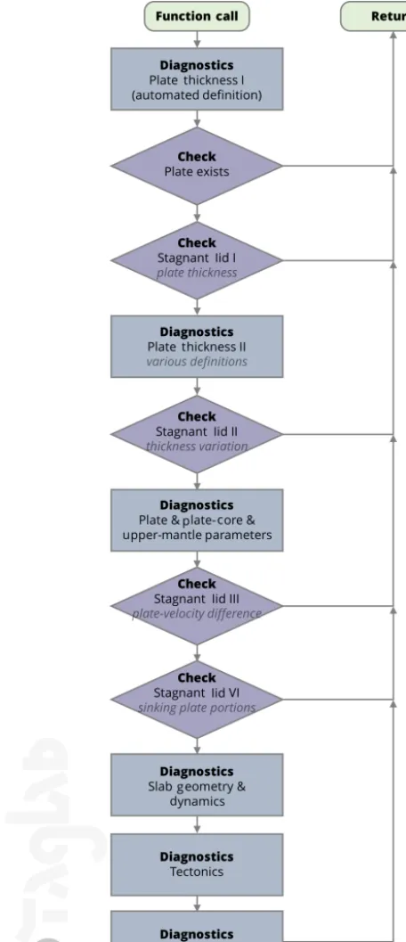
Figure 1.Flow chart outlining STAGLAB’s plate-tectonics diagnos-tic procedure.
4. The back-arc depression (or basin) is the upper-plate depression following the island arc further away from the trench. The depression’s origin is often likely two-fold and a combination of upper-plate extension or even spreading (Karig, 1971) and dynamic coupling (via the
mantle wedge) with the sinking slab below (Crameri et al., 2017). Here, the back-arc depression depth, BAD, is defined as the difference of the maximum depres-sion on the upper plate, BAD0, with the characteristic undeflected upper-plate elevation,z4, outboard of the back arc. This is necessary due to variable, isostati-cally induced elevation differences between the upper and lower plate.
Additional diagnostics of regional surface topography at sub-duction zones can be measured. The maximum horizontal ex-tent of the back-arc depression, BADexex-tent, can, for example, be defined by the distance between the trench (x5) and the far end of the back-arc deflection,x3, away from the trench. The latter point can be approximated by scanning the deflec-tion for the one point that is still lower than twice the maxi-mum vertical variation occurring in the undeflected reference upper-plate portion. Another diagnostic is given by the vol-ume of the back-arc depression, which on a 2-D plane corre-sponds to a vertical area. It can be approximated by the area constructed by the maximum basin horizontal (x3–x4) and vertical extent (z4–BAD0). Yet another useful diagnostic is the tilt of the upper plate towards the subduction trench, as it has been shown to vary significantly during subduction evo-lution (Crameri and Lithgow-Bertelloni, 2017). The tilt can be tracked by a measure taken at a certain critical distance away from the trench. The tilt angle measurement is signifi-cantly improved (i.e. made more robust and less fluctuating) by taking a mean of multiple measurements taken just next to each other.
It is generally good practice to normalise the vertical am-plitude of the characteristic topographic points mentioned above to a characteristic plate thickness defined, for example, by the thermal lithosphere thickness. This allows for scaling the obtained results to systems with different Rayleigh num-bers and hence different plate thicknesses.
2.2.2 Topography components
In addition to the absolute surface topography, itsisostatic and the remaining, non-isostatic residual components are useful to understand the various and diverse sources of long-wavelength surface elevation. To derive these two topogra-phy components, the plate thickness,dp, has to be tracked along the horizontal extent of the model (see Sect. 2.2.3). As introduced in Crameri et al. (2017), theisostatic topography componentfor each vertical column along the model extent can be calculated using the base of the plate (e.g. as defined by a 1700 K isotherm) as compensation depth. Depending on whether the plate is denser or lighter than the mantle, it is then given by
ztopo,iso(ρp)=
(ρm−ρp)dLAB
ρp−ρair , if ρp ≤ρm
(ρm−ρp)dp
ρm−ρair , if ρp> ρm,
Table 2.STAGLAB’s main 2-D geodynamic diagnostics.
Availabilitya
Diagnostics 2-D Cartesian 2-D cylindrical 3-D Cartesian (2-D modeb)
Topography
Regional characteristics X X X
Isostatic topography component X X X
Residual topography component X X X
Plate
Convergent-boundary tracking X X X
Divergent-boundary tracking X X X
Plate thickness X X X
Plate-core stress X X X
Plate-core strain rate X X X
Max. depth of plastic failure X X X
Subduction kinematics X X X
Subduction polarity X X X
Subducting plate age at trench X X X
Subducting plate bending X X X
Subduction flow rate X X X
Plate bending dissipation X X X
Overriding plate tilt X X X
Spreading kinematics X X X
Slab
Slab viscosity X X X
Slab–mantle viscosity contrast X X X
Slab-tip depth X X X
Shallow-depth slab dip angle X X X
Slab-sinking velocity X X X
Slab water retention X X X
Mantle
Mantle transit time X X X
Upper-mantle viscosity X X X
Mantle-plume tracking X X X
Active vs. passive upwelling–downwelling X X X
Total upwelling–downwelling volume X X X
aAt the time of submission.bDiagnostics performed on a vertical cross section through a Cartesian 3-D model.
withρpas the vertically averaged plate density at each hor-izontal point in space,ρmthe horizontal mean upper-mantle density just below the plate and away from any sinking slab,
ρair the air density,dLAB the variable thermal lithosphere– asthenosphere boundary (LAB) depth as defined, for exam-ple, by a 1700 K isotherm along the model, anddpthe vari-able plate thickness at each horizontal point in space that in-cludes surface topography and so is the thickness between the rock–air interface and the base of the plate.
Crucially, the resulting isostatic topography component has to be normalised throughout the model to produce a mean topography that corresponds to the sea level according to
ztopo,iso,0(x)=ztopo,iso(x)−
ztopo,iso
, (5)
withztopo,iso
as the mean of the model-wide isostatic topog-raphy component andx as the horizontal coordinate. This therefore ensures that both the conservation of volume in an incompressible mantle and the coherence of the surface plate are accounted for.
The residual topography component corresponds then simply to the non-isostatic part of the topography and is given by
iso-Table 3.Necessary fields for STAGLAB’s core geodynamic diagnostics∗.
Necessary parameter fields∗
Diagnostics Temperature Velocity Density Viscosity Composition Stress Strain rate Topography
Topography components
Plate-boundary tracking
Plate viscous dissipation
Subducting plate age at trench
Plate-bending dissipation
Slab tracking
Slab water retention
Mantle-plume tracking Active vs. passive upwelling–downwelling
– Necessity for diagnostics.– Improves the diagnostics without being a necessity.∗– At the time of submission.
static dynamics. It is important to point out that it can, how-ever, be caused not only by dynamic sources from within the convecting mantle below, but also from sources (e.g. hori-zontal tectonic forces) within the plate itself.
2.2.3 Plate thickness and plate-core depth
An estimate of the plate thickness can be derived using tem-perature isotherms (generally the 1600 K isotherm) accord-ing to the thermal-lithosphere definition. A maximum depth limits the derived plate thickness at subduction zones, where the plate and hence the isotherms bend downward into the mantle. By definition, this approach simultaneously allows us to track the lithosphere–asthenosphere boundary and its topography.
Another more widely applicable option is to derive the plate thickness automatically from individual radial profiles of temperature (or viscosity). Since a typical plate cools via diffusion, the local temperature profile (nearly) linearly de-creases throughout the boundary layer (from top to bottom) and becomes (nearly) isothermal in the convecting mantle be-low. The transition from diffusion-dominated to convection-dominated cooling is marked by a characteristic sharp bend in the profile. The bend in the profile can be tracked automat-ically by scanning for it from top to bottom. This gives an estimate of the local plate thickness, or a mean plate thick-ness, when performed on a horizontal mean (i.e. root mean square) temperature profile. The plate-core depth lies then simply about half-way down between the surface and the plate base. This depth is particularly useful to robustly track plate velocities and other similar characteristics.
2.2.4 Stagnant-lid diagnostics
Checking for a stagnant lid (i.e. the absence of subduction) can be done using a combination of tests. Key indicators for a stagnant lid are a low overall plate-thickness variation, a low maximum plate thickness throughout the model domain (i.e. no incipient subduction zone), the lack of cold lithosphere in the upper mantle (i.e. no mature subduction zone) and a
low relative motion within the surface plate (a stagnant lid is mostly rigid).
If a stagnant lid is present, various diagnostics can be performed. Stagnant-lid diagnostics include, for example, the maximum plate stress, the maximum depth of plastic failure (i.e. brittle or ductile yielding) and the lithosphere– asthenosphere boundary topography. The two latter physical complexities have been shown to be a reliable indicator of subduction initiation (Crameri and Tackley, 2016).
2.2.5 Plate-boundary tracking
Using advanced routines, converging and diverging plate boundaries can be tracked robustly and fully automatically. A basic, first-order plate-boundary tracking can already be achieved by diagnosing temperature and velocity fields only. A plate-boundary tracking routine can, however, be im-proved when additional parameter fields are considered (see Table 3).
To robustly find converging and diverging plate boundaries (i.e. subduction trenches and spreading ridges) within a 2-D model at a given point in time, a quite elaborated procedure is necessary (see Fig. 1). Several checks need to be performed initially to exclude the presence of a stagnant lid and thus the absence of subduction or spreading zones (see Sect. 2.2.4). If a stagnant lid is ruled out, potential plate boundaries can be located. Finding plate boundaries robustly necessitates find-ing all sharp and diffuse plate boundaries, findfind-ing the exact location at the very plate surface (e.g. the outcropping of the subduction fault) while accounting for plate topography and preventing multiple tracking of one and the same plate boundary.
Figure 2.Deriving the regional topographic characteristics at a subduction zone, which are from the subducting plate (right) towards the overriding plate (left) viscous fore-bulge (FB), subduction trench (TR), island arc (IA) and back-arc depression (BAD). Additional diagnostics explained here are the shallow-depth slab dip,θ, taken at the depthz5, and the bending radiusRBderived by fitting a circle to the point of maximal plate bending. See text and Table 1 for more details (figure reproduced from Crameri et al., 2017).
sharp boundaries accurately and not miss diffuse boundaries, critical values for the velocity change across plates and the horizontal distance between the measurement points need to be quite conservative (i.e. a low-velocity change measured far apart from the boundary). To not lose accuracy on the lo-cation, best practice is to start with a conservative check and gradually make critical values more restrictive to the point shortly before the boundary is not detected any longer.
The plate velocity at different depth levels inside the plate (e.g. at the plate surface and plate core; see Sect. 2.2.3) can be used to distinguish between shallow and deep plate bound-aries, and their horizontal offset additionally serves as an in-dicator of the polarity of the subduction system.
2.2.6 Plate velocities
By knowing the location of plate boundaries, the velocities of the converging plates can be diagnosed. Plate velocity is best measured in the cold, strong core of the plate(s) (see Sect. 2.2.3). Thesurface-plate RMS velocityis, for example, measured along the plate core. The individual plate velocities at convergent and divergent boundaries are then additionally most representative when measured close but not too close to the trench and ridge, respectively. These measurements then yield convergence and divergence rates. Once the subduction polarity is found (see Sect. 2.2.8), the upper and lower plate can be distinguished, and the trench velocity can be mea-sured simply by the velocity of the upper plate just next to the trench. For comparison to the effective trench retreat, a the-oretical trench velocitycan be calculated during any given subduction phase. Assuming a non-deformable slab (which is not always the case), the current trench velocity can be
approximated by
vTR,theoretic=
vStokes
tanθ , (7)
wherevStokesis the vertical sinking velocity of the slab and
θ is the shallow-depth slab dip angle (e.g. Capitanio et al., 2007).
2.2.7 Plate age
A theoretical subducting plate age,aPlate,theoretic, at the
sub-duction trench can be derived by making use of the theory of the half-space cooling model as
aPlate,theoretic=
hLP 2.32
2
κ , (8)
where hLP is the thickness of the subducting plate at the trench andκ is the thermal diffusivity (Turcotte and Schu-bert, 2014).
2.2.8 Slab-dynamics diagnostics
The currentslab-tip depthcan simply be tracked using the deepest point in a temperature contour outlining the cold ma-terial of the sinking plate. It can be refined by taking not the deepest point within the contour, but the point inside the con-tour that is the farthest away from the trench, as the slab tip usually is.
If the subduction polarity is found, theshallow-depth slab dip,θ, can additionally be measured between these two depth levels,z5A=1.25dpandz5B=7/4z2, wheredpis the mean lithosphere thickness away from the subduction zone. This results in a measuring depth,z5, for the slab dip angle located just below the lithosphere (see Fig. 2) according to
z5=z5A+
z5B−z5A
2 . (9)
The minimum, maximum and meanslab viscositycan be automatically derived using a specified area inside the slab. This area can be set in such a way that it spans the points out-lining the sinking plate that lie within a square box around the point of maximal slab bending (see Sect. 2.2.9). If for some reason this method fails, the slab viscosity can instead be de-rived by spotting the coldest portion inside a sinking slab at a depth level below the surface plate. There, a small region surrounding the coldest spot is checked for the mean, the minimum and maximum viscosity. Depending on the task, either the mean value (e.g. for the indication of absolute slab viscosity) or the minimum value is more useful (e.g. for the calculation of bending dissipation; see Sect. 2.2.10).
Theslab–mantle viscosity differencecan be derived from the minimum viscosity found in the slab (as outlined above) and the viscosity found in the surrounding upper mantle. The upper-mantle viscositycan be approximated by the horizon-tal median of viscosity found in the upper mantle below the plate. As such the anomalously high viscosity of the few cold regions (i.e. the sinking slabs) are weighted much less than the viscosity of the more common hot mantle surrounding them. The slab–mantle viscosity difference, 1ηLA, is then the difference between slab and mantle viscosity.
The slab sinking rate,vSlab, is simply extracted using the vertical velocity measured atz5B. An approximation of the total amount of water transported to the mantle can be cal-culated using the scaling law of Magni et al. (2014). The theoretical total water retention,W (kg m−2), of the slab is then
W =(1.06vSlab+0.14aSlab−0.023TMantle+17)105, (10) where vSlab (cm a−1) is the sinking velocity of the slab,
aSlab=aPlate,theoretic (Ma) is the age of the slab andTMantle (◦C) is the potential mantle temperature.
2.2.9 Plate bending
The subduction bending radius,RB, can be fully automati-cally calculated using the current plate geometry. A spline method with temperature contours can be used to outline the subducting plate shape (see Petersen et al., 2017, for other methods). A certain temperature threshold thereby ex-tracts cold plate portions including a sinking slab if present. Extracting the lowermost points in every horizontal column along the numerical grid then marks the down-going plate
and simultaneously removes any non-subducting plate por-tions. The resulting band of points then needs to be fitted using a smoothing spline. This provides a line to represent the down-going plate geometry. The local curvature,Rcurv, along the line over its whole width is given by
Rcurv(x)=
1+dz dx
23/2
d2z dx2
, (11)
with dx and dyas the incremental spatial change in the line at the horizontal location,x, in thexandzdirection, respec-tively. The minimum plate-bending radius at the kink of the subduction zone,RB (see Fig. 2), corresponds then simply to the maximum bending found along the considered plate portion and is thus
RB=min [Rcurv]. (12)
2.2.10 Viscous bending dissipation
Theviscous bending dissipationwithin the lithosphere at a subduction zone can be calculated using the above definition of the subduction bending radius. Conrad and Hager (1999) provide an approximation for the viscous bending dissipation for the case of a purely viscous plate. Including the additions outlined in Buffett (2006) to consider a visco-plastic plate and neglecting dissipation in the subduction channel, the vis-cous dissipation is finally given by
φLvd=Clvpσy,p d2
s
RB
, (13)
withCl=1/6 as a constant,vpas the lower-plate velocity,
ds the slab thickness andσy,pas the maximum yield stress within the bending portion of the plate. The lithospheric bending dissipation,φLvd, can be normalised using a certain value,φLvd,charin W m−1, to a normed value
φLvd,norm= φ
vd
L
φLvd,char. (14)
2.3 Mantle-flow diagnostics
This second suite of more specific diagnostics focuses on the mantle dynamics operating in a planet’s interior. The ma-jor diagnostics are outlined below and focus on the discrim-ination between active and passive upwellings and down-wellings and the tracking of active mantle plumes.
2.3.1 Upwellings and downwellings
Figure 3.STAGLAB’s plots showing a mantle convection model in 2-D cylindrical geometry for(a)temperature and(b)diagnosed active and passive upwellings and downwellings.
regional flow is thermally self-driven (i.e. active) or induced (i.e. passive). This task can be achieved using the actual flow field (i.e. velocity) and one kind of regional mantle residual temperature (see Sect. 2.1.3). The latter provides information on whether a patch of material is more or less buoyant than its direct surroundings.
2.3.2 Mantle-plume tracking
Mantle plumes can be tracked using the information out-lined above about active upwellings and downwellings and a plume-tracking algorithm based on the one described in Labrosse (2002). Mantle plumes are here defined (and tracked) as hot or cold upwellings or downwellings that emerge and are connected to either of the two (hot or cold) boundary layers of the convecting flow (i.e. mantle). Hot and cold temperatures are marked as anomalies when the tem-perature at a given location exceeds a certain threshold (fhot orfcold) in the range between the horizontally averaged tem-perature (Tmean) and the maximum (Tmax) or minimum (Tmin) temperature at a given depth level (z) according to
TA,hot(z)=Tmean(z)+fhot[Tmax(z)−Tmean(z)], (15)
TA,cold(z)=Tmean(z)+fcold[Tmin(z)−Tmean(z)], (16) where for hot anomalies, a threshold offhot=1 (orfhot=0) defines anomalies that are 100 % (or 0 %) hotter than the hor-izontal average in the possible range between the mean and the maximum temperature. Once all the anomalies are lo-cated, they are checked for their connection to their respec-tive boundary layer by a classical image processing proce-dure searching for connected pixels in a matrix (e.g. Kovesi, 2000). The hot and cold thresholds can thereby be chosen separately.
2.4 Field-variation diagnostics
Histogram plots of the variation in a specific field along a specified horizontal surface can prove very useful to get in-sight into the statistical physical behaviour of the state of a geodynamic system like the Earth’s mantle (e.g. Fig. S1 in the Supplement). These statistics can provide mean and median values as well as the standard deviation of the pa-rameter field under consideration. This kind of diagnostic can not only be applied to a perfectly horizontal surface, but also along a vertically slightly variable surface like along the surface-plate core. This enables, for example, the diagnostics of the strain-rate distribution within the surface plate(s).
3 Scientific visualisation
It is important to note that the key purpose of scientific visu-alisation is not about making data look pretty or entertaining; it is about creating comprehension and about delivering in-sight (e.g. Tufte et al., 1998). Unfortunately, there is not one single right way of visualising scientific data, but there are certain important ways to improve the presentation of scien-tific data and – crucially – there are several severe pitfalls that have to be prevented when doing so (e.g. Rougier et al., 2014). Here, I outline the unpleasant implications when us-ing a non-scientific colour map (likerainbow), introduce a novel set of reliable, scientifically tested colour maps and outline additional ways to improve the positive impact of sci-entific figures.
3.1 Colours
phys-ically based colour schemes that disregard the human eye’s uneven colour perception (or its most-common mutations) most likely have multiple serious drawbacks. Therefore, they should be fully avoided by the science community (includ-ing authors and journals). Unfortunately, such colour maps are still widely and frequently used, even in high-impact sci-entific publications. I will therefore outline the most severe problems of unscientific colour schemes below and provide a novel set of ready-to-use, scientific quality alternatives. 3.1.1 Unscientific colour schemes
Using fancy colour schemes incorporating the whole colour range is appealing: they look peppy and have a lively appear-ance with their varying contrasts and multiple colours. Ad-ditionally, their main representative, therainbow(a.k.a.jet) colour map, was and in some visualisation programs still is the default. These unscientific colour maps are thus widely blindly applied by authors while rarely criticised by review-ers and editors.
A colour scheme is unscientific as soon as it features one of the following aspects.
1. Both red and green colours: various forms of colour de-ficiencies can exist in human eyes, some of which make, for example, green and red undistinguishable.
2. Multiple different colours with similar lightness: colours like red, green and blue with similar lightness cannot be readily ordered against one another (e.g. from low to high values).
3. No gradual lightness gradient: a lack of a constant light-ness gradient (from light to dark or vice versa) makes a colour map unreadable when printed in black and white. 4. No perceptual uniformity: perceptually non-uniform colour maps cause different parts of the data to be weighted differently (see Fig. 5). The green–cyan part of the colour spectrum has a lower contrast to the hu-man eye than the yellow–red part. The greenish colours therefore hide low-amplitude data variation compared to reddish colours that amplify them.
Whether colours make a figure confusing or even unread-able to colour-blind people or whether colours introduce dra-matic visual artefacts (see e.g. Light and Bartlein, 2004; Bor-land and Ii, 2007, and Fig. 5), the figure surely cannot be considered suitable for science any longer. In fact, apply-ing the most moderate form of the commonly usedrainbow colour map introduces an estimated error (calculated from the change in CIE76 lightness along the colour map) to the represented underlying data of up to the staggering amount of 7.5 % (see Fig. 5).
The misleading widespread view that visualisation is not an important part of science and thus also not worth spending time and money on (e.g. for external visualisation expertise) is therefore fundamentally wrong.
Figure 4. The novel set of scientific colour maps (Crameri, 2018) used in STAGLAB is freely available online (http://www. fabiocrameri.ch/colourmaps, last access: 25 June 2018) in all ma-jor data formats and including the individual colour-map diagnos-tics that are performed using MATLAB software by Peter Kovesi (Kovesi, 2017). The colour maps, includingdevon,davos, oslo andbroc, are all perceptually uniform and prevent distorting the data visually. The suite additionally includeslapazandroma, sci-entific versions to replace the widely used unscisci-entificrainbowand seiscolour maps, andoleron, a scientific Earth-topography colour map to be used zero centred at sea level.
3.1.2 Scientific colour schemes
Useful and clear guidelines on what colour schemes to use and how to judge a given colour map have already been pro-vided elsewhere in detail (e.g. Healey, 1996; Kelleher and Wagener, 2011; Silva et al., 2011). The most important points for choosing a suitable colour scheme can be summarised as follows.
1. Perceptual order: the different colours of a colour bar should be perceived as having the same order as the rep-resented numerical values. A temperature scale should, for example, be represented by using the notions of cold and warm colours (and their proportional mixtures). 2. Uniformity and representative distance: two colours
dis-Figure 5.The visually introduced error to the underlying data. A commonrainbow(a.k.a.j et) colour map hides low-contrast variations in the cyan–green part and amplifies it unnaturally elsewhere as highlighted by low-amplitude ripples in the two large colour bars (after Kovesi, 2015). CIE76 lightness variations along the standardrainbowcolour bar (Kovesi, 2017) introduce a significant error of 7.5 % across the colour bar range to the underlying data, while the error of the perceptually uniform colour mapdavos(Crameri, 2018) is only 1.6 % locally. The impact of the much higher visual error is dramatic and can be seen by a slight shift of colour bar limits: while the same data look factually the same with the scientificdavoscolour map, the unscientificrainbowcolour map introduces strong artificial boundaries and distortion to the underlying data.
tinguishable colours, and closer values must be repre-sented by colours perceived to be closer.
3. No artificial boundaries: if there are no boundaries in the represented numerical values, the colour scale should not create boundaries, but should rather look continuous.
4. Separation of bivariate information: two (or more) pa-rameter fields represented in the same figure should be clearly separated by two clearly different colour schemes with no repeated colours.
A suitable scientific colour map makes a figure more in-tuitive and easier to understand and does not distort the un-derlying data. This can be done by adjusting a colour map to the parameter’s nature and/or to the kind of parameter vi-sualisation. Adjustment to a parameter’s nature might be to plot temperature with a blue to red colour scheme as it is in-tuitively linked to a human’s conception of hot (red) and cold (blue) as mentioned above. Adjustment to the kind of visual-isation means, for example, that low to high values might be represented by varying the colours from white (low) to red (high), while a variation between two similar colours (e.g. blue and green) might clarify displaying positive and nega-tive values around a given zero level (e.g. white).
Here, I introduce a novel set of fully scientific, percep-tually uniform colour schemes (Crameri, 2018). Crucially, these intuitive colour schemes do not distort the data; they are readable even by people with a colour-vision
deficiency; they are readable after being printed in black and white; they add no significant error to the underlying data; the scientific diagnosis of each individual colour map is provided alongside the colour map; they are available in all of the most common data formats; and they are freely available. Included in the perceptually uniform and visually appealing suite of novel colour maps shown in Fig. 4 are devon (http://www.fabiocrameri.ch/devon, last access: 25 June 2018), davos (http://www. fabiocrameri.ch/davos, last access: 25 June 2018), oslo
(http://www.fabiocrameri.ch/oslo, last access: 25 June 2018),
bilbao (http://www.fabiocrameri.ch/bilbao, last access: 25 June 2018),laj olla(http://www.fabiocrameri.ch/lajolla, last access: 25 June 2018) and a perceptually uniform ver-sion of the commongraycolour map, namedgrayC (http: //www.fabiocrameri.ch/grayC, last access: 25 June 2018). A subset of additionally included colour maps likebroc(http: //www.fabiocrameri.ch/broc, last access: 25 June 2018),
cork (http://www.fabiocrameri.ch/cork, last access: 25 June 2018) andvik(http://www.fabiocrameri.ch/vik, last access: 25 June 2018) are zero centred and hence particularly well suited for bipolar plots. The suite additionally includes
lapaz (http://www.fabiocrameri.ch/lapaz, last access: 25 June 2018) androma(http://www.fabiocrameri.ch/roma, last access: 25 June 2018), two scientific ver-sions to replace the widely used but unscientific
rainbow and seis colour maps, respectively, and
that needs to be used zero centred at sea level. All of these colour maps perform significantly better in scientific tests for, for example, uniform perception and local variations in colour contrast (Kovesi, 2015, 2017). The full suite of these novel perceptually uniform colour maps including their individual scientific test results is freely available from http://www.fabiocrameri.ch/colourmaps (last access: 25 June 2018).
3.2 Figure design
Good scientific visualisation is accurate and clear. Plots need to show all, and only, the relevant aspects like the data itself, axis ticks and labelling, clear colour bars and instructive ti-tles. Removing unnecessary clutter like duplicated labelling or unnecessary graphical forms and choosing a clear sans-serif font and a lighter (e.g. grey) colouring of axis labels does shift the visual focus onto the most important part of the plot: the data.
A visual focus is especially useful when plotting multiple subplots next to each other. Subtle visual guides (that for ex-ample group subplots or relate them to each other) can addi-tionally help the reader to understand the figure by improving its clarity. Magnifying panels can be added to provide a view on the details while not losing the big picture. Adjusting the background colour is useful to adjust the figure to fit seam-lessly into its surroundings whether this is a white conference poster or a dark presentation slide. Such visual refinements improve scientific figures and allow them to convey the pre-cious scientific data accurately in an easily understandable and visually appealing manner.
4 StagLab: the software
STAGLAB is the all-in-one, easy-to-use software that com-bines all geodynamic diagnostics (see Sect. 2) and the state-of-the-art scientific visualisation (see Sect. 3) outlined above and makes them accessible to everyone, including students and inexperienced modellers. Here, I provide an overview of various aspects of the software, including some of the power-ful features, its thoughtpower-ful code design and the helppower-ful exter-nal contributions to it, and outline how easily it can be used. 4.1 Supported model data
STAGLABis optimised for the geodynamic finite-difference code StagYY (Tackley, 2008) but is easily made compatible with other codes. STAGLABhas, for example, already been used with 2-D output from the finite-element code Fluidity (Davies et al., 2011) that, in contrast, employs an unstruc-tured numerical discretisation (see Supplement Fig. S2).
The data input for parameter fields simply has to be im-ported to MATLAB and subsequently needs to be adjusted to match the format outlined in STAGLAB’s input routine
f_readOt her.
4.2 StagLab features
The STAGLAB user receives constant support from a built-in, friendly artificially intelligent operator,fAIo. It facilitates finding input data across unspecified folders and file num-bers, facilitates saving figures and movies while preventing overwrites of existing files, prevents unnecessary errors dur-ing execution, ensures unbroken forward compatibility of previously used parameter files and keeps STAGLAB itself up to date. In the following, I list the key features that lie at the feet of such a streamlined user experience that make STAGLAB truly boost existing geodynamic models and the research behind them.
4.2.1 Dimensional scaling
For performance reasons, numerical models are often run using non-dimensional numbers. If a geodynamic code can be run in both dimensional and non-dimensional mode, STAGLAB will account for that by checking if the data files are dimensional or not and adjusts the di-mensions fully automatically. Moreover, STAGLAB offers the possibility to convert non-dimensional values into sen-sible dimensional numbers using its Dimensional mode (SWITCH.DimensionalMode). A given set of dimen-sionalisation parameters can be defined in the function file
f_Dimensions and then referred to by setting the corre-sponding flag to the variableIN.Parameterin the param-eter files.
4.2.2 Automated geodynamic diagnostics
STAGLAB’s incredible diagnostic capabilities (see Sect. 2) decipher geodynamic models within a fleetingly brief time span. In fact, performing the whole suite of plate-tectonics diagnostics listed in Table 2 with STAGLAB3.0 within less than 2.2 s for a high-resolution (512×256) 2-D model on a power-efficient laptop (1.3 GHz processor; 8 GB RAM) is record breaking if not revolutionary. During this fleetingly short time period, real-time output is provided listing the most important model details and diagnostics and, in the case of problems, instructive warnings and error messages.
The real power of STAGLAB’s geodynamic diagnostics lies, however, not only in its speed itself, but rather in the combination of both speed and robustness. Given the enor-mous variety occurring in a geodynamic system and related numerical models, STAGLAB’s diagnostic routines have been trained excessively to become incredibly robust (see e.g. Fig. 6).
4.2.3 Plot and figure design
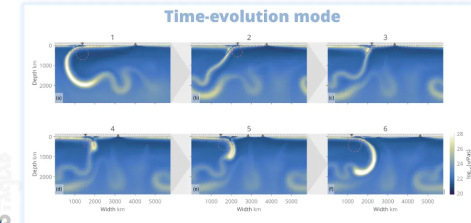
geome-Figure 6.Time evolution of 2-D Cartesian mantle convection using STAGLAB’sTime-evolution modehighlighting the accuracy and ro-bustness of the plate-boundary tracking algorithm even throughout a dramatic subduction-polarity reversal (figure adjusted from Crameri and Tackley, 2015).
tries. The 3-D data can be represented with both 2-D slices (in any direction normal to a side boundary) or with 3-D iso-surfaces. For Cartesian models these two methods can even be combined into one figure. For 3-D spherical model data, STAGLABadditionally offers a large variety of map projec-tions.
STAGLAB’s visualisation routine is trimmed for accu-racy, clarity and simplicity. Plots produced with STAGLAB show all the relevant data like axis ticks and labelling, clear colour bars and instructive titles. On top of that, STAGLAB offers two plotting modes, Analysis mode (SWITCH.AnalysisMode) to carefully examine the data and Publication mode (set as default) to clearly present the data (Fig. 9). Analysis mode offers detailed information and has refined axis ticks and more labels. Publication mode shifts the focus from the information surrounding the data to the data itself and labels subplots automatically to be eas-ily referred to. This is achieved by removing unnecessary (e.g. duplicated) labelling, the choice of a well-readable and larger sans-serif font and a less distracting grey colouring (see Sect. 3.2).
STAGLAB makes plotting multiple subplots straight-forward, while keeping the figure clear and focused. To compare different experiments, STAGLAB fully automatically adds subtle visual background guides (SWITCH.BackgroundGuides), areas that visually combine subplots of the same experiment, while sep-arating them visually from the other experiments (e.g. Fig. 10). A similar example is the Time-evolution mode
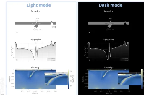
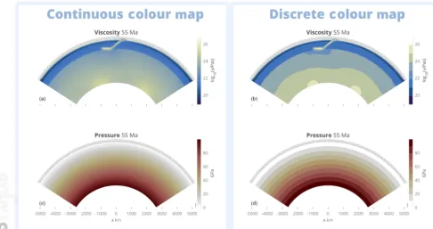
(SWITCH.TimeEvolutionMode) that adds time arrows to highlight the temporal evolution from one sub-plot to another (Fig. 6). To highlight smaller areas in a subplot and enlarge important details, magnifier panels (SWITCH.Magnifier) can be added to plots (e.g. Fig. 7c). STAGLABhas a convenient option to use a discrete colour map (SWITCH.DescreteColormap) that can help to outline regions of similar values more clearly (Fig. 8). Finally, a stunning Dark mode (SWITCH.ColorMode) can be switched on, which inverts relevant colours of the figure to be presented on a black background (Fig. 7). Dark mode is particularly useful to display STAGLABfigures on screens and via projectors. It is worth mentioning that all of these options and modes can be individually put into action with one single, simple switch. Moreover, options like these crucially enable STAGLAB figures to convey scientific data accurately and clearly, while still being visually appealing to the reader.
4.2.4 Plot types
Figure 7. STAGLAB’sDark modeand geodynamic diagnostics. While the defaultLight modeis intended for publications and poster presentations, Dark mode is particularly useful for digital presentations on screens. STAGLAB’s diagnostics highlighted here include slab-tip depth (red cross), isostatic and residual topography components (dashed and dotted grey lines, respectively), plate-boundary tracking (white and grey rectangles), minimum plate-bending radius (red–white dashed circle) and resulting plate-bending dissipation. Geodynamic diagnostics like these foster a better understanding of complex models.
saved geodynamic diagnostics against each other or time (e.g. trench location, plate velocities, etc.; see Sect. 4.2.5). Moreover, STAGLABproduces a variety of additional useful plot types that are listed below.
1. Grid(PLOT.Grid): the grid can be plotted separately or as an addition to a parameter field. This is particularly useful to check physical features against grid resolution or to highlight the grid’s spatial variation. The grid lines can be plotted in actual resolution or coarser if the grid is too fine to be resolved with the given figure resolu-tion.
2. Tracers(PLOT.Tracers): individual tracer informa-tion, like the tracer position and type, can be visualised in a separate plot.
3. Streamfunction (PLOT.Streamfunction): there is an option to visualise the flow field in a separate plot or on top of any other field in the form of flow contours. This is a useful way to show the pattern and spatial ex-tent of mantle flow cells.
4. Streamlines (PLOT.Streamline): instantaneous streamlines can be plotted on top of another parameter field or as a separate plot to highlight the flow pattern of individual particles.
5. Quiver(PLOT.Quiver): the option to plot distributed velocity arrows on top of any parameter field adds the possibility to highlight the flow direction and relative strength. The amount and scaling of velocity arrows can be adjusted manually if needed.
6. Surface-field variation
(PLOT.SurfaceFieldVariation): any field vari-ation across a horizontal surface can be plotted sepa-rately as a histogram plot (see Supplement Fig. S1). 7. Plate sketch (PLOT.PlateSketch): STAGLAB has
Figure 8.STAGLAB’s continuous(a, b)versus its discrete(c, d)colour-map option that is useful to better convey the actual field value in a certain region shown for a model in partial-cylinder geometry.
specified other diagnostics like lithospheric bending dis-sipation or slab dip.
8. Parameter table (PLOT.ParameterTable): the possibility to add a table to the figure is helpful to high-light a specified selection of the numerous diagnostic variables obtained in STAGLAB.
4.2.5 Output files
STAGLABproduces publication-ready figure files in a variety of data formats. The available options include .jpg, .png, .eps and .pdf file formats, whereas the .png format is most rec-ommended and hence the default: high-resolution .png files are a good option for publication because .png is a commonly used and accepted figure file format and has a relatively small file size. True vector graphics such as .eps are limited to sim-ple graph plots as contour plots would lead to an excessively large file size. The resolution of an output figure file can be adjusted in the parameter file if necessary.
STAGLAB produces publication-ready movie files in a variety of data formats. Movies of, for example, time-dependent numerical models are increasingly published alongside the publication paper as most scientific journals of-fer the option to add online supplementary files. Movies are particularly helpful to investigate the temporal behaviour of a system. STAGLAB can therefore also produce movie files created of multiple MATLAB figure frames. Available file formats are .avi, .mj2, .mp4 and .m4v.
STAGLABproduces post-processed data files in a variety of data formats. This might be useful to save a post-processed parameter field or simply to convert a field from one format to another. Available file formats are here .mat, .dat and .txt. Particularly useful is the option to save a large variety of geo-dynamic diagnostics to data files. The diagnostics that can currently be saved are listed in Supplement Table S1. Hav-ing these data files is particularly useful to plot temporal (or other) graphs including some of the diagnostic data using the option to plot this STAGLABdata (see Sect. 4.2.4).
4.3 Software design
vari-ables (e.g. Supplement Fig. S3) and time-evolution graphs of globally averaged variables (e.g. Supplement Fig. S4), re-spectively. The parameter file allows users to change chosen parameters and switches to be different from the default set-ting. As such, a STAGLAB procedure is fully reproducible by saving a used parameter file, even after updates to the core routines as the parameter files in STAGLABare forward com-patible. Moreover, STAGLABis extensively tested and heav-ily optimised for efficiency, which speeds up both computa-tion and, crucially, also the research process as a whole (see Sect. 4.3.6). It also makes elaborated diagnostics and state-of-the-art visualisation easily accessible to everyone (includ-ing students and inexperienced modellers). And, last but not least, the geodynamic post-processing routines are fully open source.
4.3.1 External contributions to StagLab 3.0
STAGLABcalls the routinef_readSt agY Y.mthat was orig-inally written by Boris Kaus to read StagYY’s binary output directly into MATLAB. The routine f_Y Y t oMap, which was originally written by Paul Tackley, is used to produce horizontal maps of fully spherical yin–yang data. The origi-nal routinef_readF luidity to read Fluidity data was pro-vided by Fanny Garel. It further uses the figure-saving rou-tine export_f ig, which was originally written by Oliver Woodford, the routine f lowf unoriginally written by Kir-ill K. Pankratov to derive the stream function, the rou-tineMinV olEllipseby Nima Moshtagh to fit a minimum-volume ellipse around a point cloud, the routineplot boxpos
by Kelly Kearney to derive the plot position more accurately, the routinehat chf ill2 originally developed by Neil Tandon to fill areas with a specific texture and a few routines includ-ing equalisecolourmap, sineramp2, normalise, show
andst rendswit hdeveloped by Peter Kovesi to provide the scientific colour-map diagnostics.
4.3.2 Accuracy
STAGLAB is built for accuracy. Its automated diagnostics (see Sect. 2) offer more accuracy than interpretations by hand as they are based on quantitative measures rather than on vi-sual impression. In order to maintain the high accuracy all the way into the data representation, perceptually uniform colour maps (see Sect. 3.1.2) are applied to additionally minimise the visually introduced error.
4.3.3 Flexibility
STAGLAB is built for flexibility. Its fully customisable pa-rameter files contain a wealth of options (i.e. switches) to ad-just post-processing and visualisation. Data from all model geometries, ranging from simple 2-D Cartesian to 3-D fully spherical, can be processed (see Sect. 4.2.4). Various plot ad-ditions like velocity arrows, streamlines or isolines can be added on top of other parameter fields (see Sect. 4.2.4). An
automatic subplot arrangement enables direct comparisons between outputs from different time steps or even experi-ments.
4.3.4 Reproducibility
STAGLABis built for reproducibility. The customised param-eter files, from which any STAGLABprocedure is executed, are forward compatible and can be stored in and run from any possible directory. Given that a previously used parame-ter file is safely stored, it can therefore be reused at any time with any forthcoming version of STAGLABand so reproduce previous geodynamic diagnostics and visualisations. There-fore, any work done with STAGLAB is and always will be fully reproducible.
4.3.5 Continuity
STAGLABis built for continuity. Old parameter files are, on the one hand, always updated to be compatible with the lat-est version of STAGLAB, fully automatically and fully ef-fortlessly. On the other hand, STAGLAB itself will be kept compatible with the latest versions of MATLAB.
4.3.6 Efficiency
STAGLABis built for efficiency. A wealth of most common post-processing and visualisation tasks are just a click (and a few seconds or less) away. Crucially, STAGLAB diagnos-tic and visualisation tasks can be quickly reproduced when going through the common, improving iterations during the research progress. This keeps the time-consuming coding ef-fort for producing, adjusting and updating the core software to a minimum.
In addition, STAGLABitself is trimmed towards efficient computation. Time-consuming parts of the software are op-timised by, for example, the vectorisation of loops as well as the efficient reading and transferring of large data structures. It can thus quickly handle the huge amount of data resulting from high-resolution 2-D and 3-D models. A useful perfor-mance switch is built in that allows users to reduce the file sizes of extremely large data files for quicker visualisation (SWITCH.ReduceSize). Another option, Quick mode (SWITCH.QuickMode), allows for an extra quick execu-tion to ensure efficient post-processing throughout multiple time steps and files.
4.3.7 Reliability
Figure 9.STAGLAB’sAnalysis mode(left) andPublication mode(right). While in Analysis mode as much detail as possible is provided to facilitate the examination of the data, the data (i.e. the key result) are put into focus and fully annotated in Publication mode.
Figure 10. STAGLAB’s figure design routine turns overloaded data representation (left) into clear and focused visualisation (right) using various figure simplifications, while subtle visual guides make comparisons between a large number of models or model time steps easily understandable (figure adjusted from Crameri and Lithgow-Bertelloni, 2017).
and should be sent to the author to ensure future reliable re-leases of STAGLAB. However, it has to be noted that since a fully bug-free software cannot be guaranteed, the scientific quality check always remains with the user.
4.3.8 Simplicity
parameter files combining all the important switches in one place. The parameter file is clearly structured and can be reduced to only the routinely used switches thanks to hav-ing defaults to every individual switch. Ushav-ing the parameter files ensures a streamlined usage even for complex figures. STAGLAB returns selected, clear and informative real-time output in MATLAB’s terminal window during its operations. The display messaging allows users to monitor STAGLAB’s progress, receive both scientific diagnostics and, in the case of problems, clear warnings thanks to its advanced error mes-saging system. The advanced error handling implemented in STAGLAB often prevents interruption during execution and displays warnings instead. An optional Verbose mode (SWITCH.Verbose) allows users to display more detailed information during the STAGLAB execution, which simpli-fies the debugging procedure. STAGLABcrucially simplifies the reading and saving of data files: an advanced file finder automatically checks for other possible file directories or the latest file number if the specified files are not found initially. Finally, STAGLAB itself is written carefully with a unified code structure and descriptive comments to simplify further code development.
4.3.9 Open source
STAGLAB is open access and currently only requires a valid MATLAB license. Apart from the design routines, all STAGLAB files are additionally fully open source. Free usage and redistribution of STAGLAB and its indi-vidual routines and colour schemes, however, fall under the Creative Commons Attribution 4.0 International Li-cense (https://creativecommons.org/liLi-censes/by/4.0/, last ac-cess: 25 June 2018).
4.4 Using StagLab
STAGLAB’s software design aims towards an effortless user experience (see the Supplement user guide). Its application is simple and hence accessible to experienced numerical mod-ellers as well as fresh beginners. Using STAGLAB is an in-credibly efficient and motivating way, for students especially, to enter the world of numerical modelling, but also opens up new exciting doors for more experienced scientists through its incredible flexibility.
4.4.1 Prerequisites
STAGLABis compatible with all three major operating sys-tems running on Mac, Linux and Windows PC. It has been updated to the latest graphical improvements made to MAT-LAB and therefore performs best with the latest MATMAT-LAB version. Although it can function with older versions, MAT-LAB version 8.4.0 (i.e. MATMAT-LAB 2014b) or higher is neces-sary for many core functions and thus highly recommended. Although a set of parameter-field data is necessary to use all the post-processing routines built into STAGLAB, it can
already function with just a temperature field or any other single field that has to be processed. To complete more de-manding tasks like plate-boundary tracking, more fields like temperature, velocity and topography are necessary.
STAGLABperforms a local directory search for the spec-ified input file in case the file cannot be found directly. It also checks for the specific folder structure (based on StagYY’s native folder structure) consisting of an image folder “.../<folder>/+im” containing the image files and an output folder “.../<folder>/+op” containing the (e.g. binary) output data files. Using default settings, STAGLAB will, in that case, look for binary data to import in “+op”, while it will save the figures to “+im”. This behaviour can, however, also be adjusted manually in the parameter file.
4.4.2 Download and installation
STAGLAB is available from http://www.fabiocrameri.ch/ StagLab (last access: 25 June 2018). An included README file (http://www.fabiocrameri.ch/resources/README.pdf, last access: 25 June 2018) provides up-to-date, detailed instructions on installing and running STAGLAB. Once downloaded, it can then be installed by adding all of its files to the MATLAB search path. This can conveniently be done by running the included installation routine,f_I N ST ALL
(Algorithm 1), which additionally checks for possible file duplications, or manually from within MATLAB (i.e. version 2014b or later).
Algorithm 1Installing command for StagLab.
>> cd <yourPath>/StagLab3 >> f_INSTALL
4.4.3 Testing
STAGLAB has a built-in testing routine, f_T EST (Algo-rithm 2), to make sure it performs as expected on the current system and to highlight some of its capabilities. It performs a suite of automated tests for STAGLAB’s core tasks and pro-duces a suite of test figures from some included data files. Algorithm 2Testing command for StagLab.
>> cd <yourPath>/StagLab3
>> f_TEST
4.4.4 Running StagLab
parame-ter files are P arSt agLab2D.m and P arSt agLab3D.m
for Cartesian two- and three-dimensional models, respec-tively, and P arSt agLabY Y.m for spherical models us-ing the yin–yang grid. The P arSt agLabRprof.m and
P arSt agLabT imedat.m are two additional example pa-rameter files to visualise either preprocessed radial profiles of horizontal mean values or the preprocessed temporal evo-lution of global mean values. The parameter files can con-veniently also only contain a few specific switches as the full set of options is included in one of the three correspond-ing files containcorrespond-ing the full default set-ups,f_Def ault s.m,
f_Def ault sRprof.morf_Def ault sT imedat.m. Old parameter files are automatically updated to be for-ward compatible with any upcoming STAGLABversion and are hence fully reusable. This ensures that any figure pro-duced with one specific parameter file remains fully repro-ducible given that a copy of the parameter file used is stored safely.
The simple STAGLABprocedure is then as follows: 0. downloading and installing STAGLABby adding all
in-cluded files to the MATLAB search path (e.g. running
f_I N ST ALL);
1. setting up a new STAGLAB parameter file with the output-data-specific settings like file name, directory, number and parameter set-up;
2. executing the STAGLAB parameter file with the user-specific switches to get publication-ready figures or movies;
3. and safe-keeping of the STAGLABparameter file to en-sure reproducibility.
4.4.5 Application examples
STAGLAB’s parameter files can consist of only a minimum number of switches despite the numerous potential switches and options. The minimal parameter file to produce a figure similar to Fig. 7 is outlined in Algorithm 3.
STAGLAB diagnostics and visualisations can be used in two ways. First, they give useful insights during the testing of potential models and set-ups. Running STAGLABin Analysis mode produces, for example, more detailed plots with more information. Secondly, STAGLABdiagnostics and visualisa-tions can be used to present and publish new scientific results in a clear and appealing manner. STAGLABhas already been used in a number of studies (Crameri, 2013; Crameri and Tackley, 2014, 2015, 2016; Crameri et al., 2017). Its fully automated diagnostics were pivotal for Crameri et al. (2017), in which it enabled a to-date unmatched extensive systematic testing of the numerous controlling subduction parameters and their impact on surface topography. Its visual represen-tation of plate diagnostics even unravelled the dramatic in-teraction of subduction-induced mantle currents and (upper-)
Algorithm 3Minimal parameter file example.
%% INPUT FILE(S)
IN.Name = { ’Case1’ };
IN.Number = [ 20 ];
IN.Parameter = [ 1 ];
IN.Folder = { ’../’ };
%% POST-PROCESSING
PLOT.indicateTrench = logical(1);
PLOT.indicateRidge = logical(1);
PLOT.indicateBending = logical(1);
PLOT.indicateSlabTip = logical(1);
%% PLOT STYLING
STYLE.ColorMode = ’dark’;
%% PLOT ADDITIONS
PLOT.Magnifier = logical(1);
%% SAVING FIGURE
SAVE.Figure = logical(1);
%% FIELDS TO PLOT
PLOT.Temperature = logical(0);
PLOT.Viscosity = logical(1);
PLOT.Topography = logical(1);
%% SPECIAL PLOTS
PLOT.PlateSketch = logical(1);
plate tilting during the short time interval when the sinking plate reaches the lower mantle (see Crameri and Lithgow-Bertelloni, 2017), a dynamic interaction that has been over-looked in numerous other similar studies for years.
5 Conclusions
Firstly, a compilation of automatised key geodynamic di-agnostics is given here. While most of these didi-agnostics have been previously established elsewhere, some others were improved here or even newly introduced. Covered are, amongst others, surface-topography component split-ting, plate-boundary identification, slab-polarity recognition, plate-bending characteristics derivation and mantle-plume detection. They all serve to offer a better understanding of complex geodynamic systems like the Earth’s mantle.
otherwise can mount up to a staggering 7.5 % across the dis-played data range, as is shown to be the case for the com-monly used rainbow colour map; this is an error that eas-ily dominates in most data sets. The novel suite of scientific colour maps, includingdevon(http://www.fabiocrameri.ch/ devon, last access: 25 June 2018), davos (http://www. fabiocrameri.ch/davos, last access: 25 June 2018),oslo(http: //www.fabiocrameri.ch/oslo, last access: 25 June 2018),broc
(http://www.fabiocrameri.ch/broc, last access: 25 June 2018) and others, presents the precious scientific data undistorted and without excluding certain readers. In an unprecedented manner, the whole suite is made freely available includ-ing all scientific diagnostics and in all major data for-mats (see http://www.fabiocrameri.ch/visualisation, last ac-cess: 25 June 2018).
Thirdly, all geodynamic diagnostics and the state-of-the-art scientific visualisation are packed into one single software package, STAGLAB, which is introduced here. STAGLABis an easy-to-use MATLAB software that significantly facili-tates post-processing and visualisation, the two crucially im-portant aspects of research. It provides a powerful, fully au-tomated and incredibly robust implementation of the geo-dynamic diagnostics outlined above. STAGLAB’s efficiency turns laborious days of post-processing towards revealing hidden model secrets into an exciting and effortless 2.2 s of pure revelation (according to the measurement outlined in Sect. 4.2.2). In the same breath, these revelations can be finely packed into a publication-ready figure or movie us-ing fully reproducible, forward-compatible parameter files, while applying state-of-the-art visualisation techniques like its unique suite of scientifically tested, perceptually uniform colour maps.
STAGLABis currently compatible with two of the widely used geodynamic codes, StagYY (Tackley, 2008) and Fluid-ity (Davies et al., 2011). In combination with StagYY out-put, it is capable of handling all different geometries (2-D and 3-(2-D Cartesian, 2-(2-D partial and full cylindrical, and 3-D spherical) and output (parameter fields, radial profiles and time-evolution data). With little effort, STAGLAB can also be adjusted to be compatible with additional mantle convection codes. The latest version of STAGLAB, freely available at http://www.fabiocrameri.ch/StagLab (last ac-cess: 25 June 2018), is a flexible, efficient, reliable and sim-ple software that produces state-of-the-art, reproducible di-agnostics and visualisation for upcoming and groundbreak-ing geodynamic models.
Code and data availability. The suite of scien-tific quality colour maps (v3.0.4) is reposited at https://doi.org/10.5281/zenodo.1287763 (Crameri, 2018). The specific full STAGLABpackage, STAGLAB3.0.3, that is discussed in this paper is reposited with example data sets included at https://doi.org/10.5281/zenodo.1287674 (Crameri, 2017b).
The Supplement related to this article is available online at https://doi.org/10.5194/gmd-11-2541-2018-supplement.
Competing interests. The author declares that he has no conflict of interest.
Acknowledgements. The author thanks Kiran Chotalia and Antoni-ette Grima for their help with debugging the code, Fanny Garel for sharing her post-processing routines for Fluidity output, Robert Pe-tersen for his help with deriving an appropriate radius of curvature for the plate bending, Tobias Rolf for his help with the histogram plot, Marcel Thielmann for his help with STAGLAB’s compatibility across different MATLAB versions and Paul Tackley for his helpful comments throughout the development of STAGLAB. The author thanks Scott King, an anonymous reviewer and Lutz Gross for their thoughtful comments and suggestions. The author acknowledges support from the Research Council of Norway through its Centres of Excellence funding scheme, project number 223272. Some of the models presented here were computed using a UNINETT Sigma2 computational resource allocation (Notur NN9283K and NorStore NS9029K).
Edited by: Thomas Poulet
Reviewed by: Scott King and one anonymous referee
References
Borland, D. and Ii, R. M. T.: Rainbow Color Map (Still) Considered Harmful, IEEE Comput. Graph., 27, 14–17, 2007.
Buffett, B. A.: Plate force due to bending at subduc-tion zones, J. Geophys. Res.-Sol. Ea., 111, b09405, https://doi.org/10.1029/2006JB004295, 2006.
Capitanio, F., Morra, G., and Goes, S.: Dynamic models of downgo-ing plate-buoyancy driven subduction: Subduction motions and energy dissipation, Earth Planet. Sc. Lett., 262, 284–297, 2007. Chandrasekhar, S.: Hydrodynamic and hydromagnetic stability,
In-ternational Series of Monographs on Physics, Oxford University Press, Oxford, 1961.
Coltice, N., Gérault, M., and Ulvrová, M.: A mantle convection perspective on global tectonics, Earth-Sci. Rev., 165, 120–150, https://doi.org/10.1016/j.earscirev.2016.11.006, 2017.
Conrad, C. P. and Hager, B. H.: Effects of plate bend-ing and fault strength at subduction zones on plate dy-namics, J. Geophys. Res.-Sol. Ea., 104, 17551–17571, https://doi.org/10.1029/1999JB900149, 1999.
Crameri, F.: The interaction between subduction-related man-tle currents and surface topography, PhD thesis, ETH Zurich, https://doi.org/10.3929/ethz-a-009954311, 2013.
Crameri, F.: StagLab: Post-Processing and Visualisation in Geody-namics, EGU General Assembly Abstracts, vol. 19, Vienna, Aus-tria, EGU2017–8528, 2017a.
Crameri, F.: StagLab 3.0.3, Zenodo,
https://doi.org/10.5281/zenodo.1287674, 2017b.