Modelling mid-Pliocene climate with COSMOS

(1)

www.geosci-model-dev.net/5/1221/2012/ doi:10.5194/gmd-5-1221-2012

Geoscientific

Model Development

Modelling mid-Pliocene climate with COSMOS

C. Stepanek1and G. Lohmann1,2

1_{Alfred Wegener Institute for Polar and Marine Research, Bremerhaven, Germany} 2_{Institute for Environmental Physics, University of Bremen, Bremen, Germany}

Correspondence to: C. Stepanek (christian.stepanek@awi.de)

Received: 19 March 2012 – Published in Geosci. Model Dev. Discuss.: 24 April 2012 Revised: 15 August 2012 – Accepted: 16 August 2012 – Published: 5 October 2012

Abstract. In this manuscript we describe the experimen-tal procedure employed at the Alfred Wegener Institute in Germany in the preparation of the simulations for the Pliocene Model Intercomparison Project (PlioMIP). We present a description of the utilized Community Earth Sys-tem Models (COSMOS, version: COSMOS-landveg r2413, 2009) and document the procedures that we applied to transfer the Pliocene Research, Interpretation and Synoptic Mapping (PRISM) Project mid-Pliocene reconstruction into model forcing fields. The model setup and spin-up proce-dure are described for both the paleo- and preindustrial (PI) time slices of PlioMIP experiments 1 and 2, and general re-sults that depict the performance of our model setup for mid-Pliocene conditions are presented. The mid-mid-Pliocene, as sim-ulated with our COSMOS setup and PRISM boundary condi-tions, is both warmer and wetter in the global mean than the PI. The globally averaged annual mean surface air tempera-ture in the mid-Pliocene standalone atmosphere (fully cou-pled atmosphere-ocean) simulation is 17.35◦C (17.82◦C), which implies a warming of 2.23◦C (3.40◦C) relative to the respective PI control simulation.

1 Introduction

General circulation models of the Earth System provide a suitable tool to understand past climates (e.g. Crowley and North, 1991). They are especially useful since they “can put numbers on ideas” (Ruddiman, 2008). Nowadays, general circulation models are commonly used for the development and testing of physical hypotheses on the quantitative func-tion of the climate system (e.g. Jansen et al., 2007). Their application allows the investigation of the climate’s reaction to changes in boundary conditions, e.g. of orbital forcing and

modifications in the distribution of ice sheets. This topic has been studied for the time slices of the mid-Holocene and the Last Glacial Maximum within the framework of the Paleo-climate Modelling Intercomparison Project (PMIP, e.g. Jous-saume and Taylor, 2000). Presently, the quantification of the amplitude of surface temperature change as a result of an-thropogenic emission of infrared-active trace gases has be-come an important field of research in climate sciences: Sim-ulations of climate scenarios for the Intergovernmental Panel on Climate Change (IPCC) with increased concentrations of atmospheric carbon dioxide are used to retrieve estimates of the changes in climate conditions, such as global mean sur-face temperature, that are to be expected in the future (e.g. Meehl et al., 2007). Particular focus is directed at the uncer-tainties in potential future temperature changes (e.g. Knutti et al., 2008).

The models are in a constant development process and have undergone major improvements since publication of the IPCC Third Assessment Report in 2001 (Randall et al., 2007). Since the design of the models is based on our knowl-edge about today’s climate, it is of particular interest with respect to the investigation of a warming climate to test the climate models on their ability to simulate climate states that differ from present-day conditions. Such quality controls for the reliability of climate simulations have been established in the form of model-data comparison studies (e.g. Lorenz et al., 2006) and model intercomparison projects (e.g. PMIP, Braconnot et al., 2007). The former type of study investigates whether models generally are capable of satisfactorily simu-lating the Earth’s climate. The latter address the question of to what extent simulations carried out with different climate models are comparable.

(2)

is undertaken in the Pliocene Model Intercomparison Project (PlioMIP, Haywood et al., 2009, 2010, 2011). Standard cli-mate models, which are widely used in clicli-mate research, are exposed to an extensive set of standardized boundary conditions of the mid-Pliocene, which have been retrieved within the framework of the Pliocene Research, Interpreta-tion and Synoptic Mapping (PRISM) Project (e.g. Dowsett et al., 1999). The mid-Pliocene is a geological epoch of the Earth’s recent history during which the continents had al-ready arrived at their present positions, but prevailing climate conditions were still warmer than today. It therefore has been suggested as a potential past analog for future warmer-than-present climates (Jansen et al., 2007), which makes it an ideal testbed for climate models in the context of a warming cli-mate.

This manuscript describes the implementation of the PlioMIP experiments that have been conducted at the Paleo-climate Dynamics section at the Alfred Wegener Institute in Germany. In Sect. 2 we present a description of the utilized climate model; Sect. 3 provides an overview of the setup of both the standalone atmosphere (experiment 1) and coupled atmosphere-ocean (experiment 2) simulations. This back-ground information serves as a prerequisite for the model intercomparison. General results retrieved from our simula-tions are presented in Sect. 4, and a brief discussion is given in Sect. 5.

2 Model description

The simulations described in this manuscript have been carried out using the Community Earth System Models (COSMOS, version: COSMOS-landveg r2413, 2009) which have been mainly developed by the Max Planck Institute for Meteorology (MPI) in Hamburg. Our version of COSMOS includes the ECHAM5 atmosphere model in T31-resolution with 19 levels, the MPI-OM ocean model in GR30 resolution with 40 levels, and the land-vegetation model JSBACH. Our setup is identical to the COSMOS-1.2.0 release, which has been developed in the Millennium project (Jungclaus et al., 2010), but additionally includes a dynamical vegetation mod-ule (Brovkin et al., 2009). In this version, COSMOS has been used for the preparation of various publications (Brovkin et al., 2009; Fischer and Jungclaus, 2010; Varma et al., 2012; Wei et al., 2012; Wei and Lohmann, 2012), but, in our ex-periment 1 and the mid-Pliocene simulation of exex-periment 2, the dynamic vegetation module has been switched off in or-der to be consistent with the PlioMIP protocol (Haywood et al., 2011).

2.1 The atmosphere model ECHAM5

The ECHAM5 model is described in detail by Roeckner et al. (2003). Based on their publication, we give here a summary of the model’s properties that might be helpful in the model intercomparison.

ECHAM5 was adapted for climate research from the weather forecasting model of the European Centre for Medium-Range Weather Forecasts (ECMWF). The model is based on a spectral dynamical core and simulates the tro-posphere and the lower stratosphere up to a pressure level of 10 hPa. The vertical dimension is organized on a hybrid sigma-/pressure-level system. In our model setup, we use ECHAM5 in T31/L19 resolution (i.e. there are 19 levels present and triangular truncation of the series of spherical harmonics is performed at wave number 31). The approx-imate horizontal resolution is 3.75◦_×₃_.₇₅◦_{, which}

corre-sponds to the setup used in the Millenium project (Jungclaus et al., 2010). The time step of the atmosphere simulation is 2400 s.

ECHAM5 uses a semi-implicit time scheme for solving the equations of divergence, surface pressure, and tempera-ture, and a semi-Lagrangian scheme (Lin and Rood, 1996) for passive tracer transport. The model employs a mass flux scheme to simulate cumulus convection. Stratiform clouds are diagnosed by means of schemes for statistical cloud cover and microphysics; also the prognostic equations for water in the fluid, gas and solid phases are considered (Roeckner et al., 2003). The orography as the lower boundary condition for atmospheric circulation in the spectral domain is defined via the surface geopotential. This quantity is calculated from a global distribution of orography and is transformed into the spectral space. Subgrid-scale orographic effects are con-sidered using a parameterization scheme, described by Lott and Miller (1997) and Lott (1999), that relies on the oro-graphic parameters mean and standard deviation of elevation, slope, anisotropy and orientation, as well as the height of oro-graphic peaks and valleys (Roeckner et al., 2003).

A high-resolution (0.5◦×0.5◦) hydrological discharge model (HD-model), described in detail by Hagemann and D¨umenil (1998a,b) and Hagemann and Gates (2003), closes the hydrological cycle. It simulates the translation and reten-tion of land-bound lateral water flows, which are separated into overland flow, base flow, and river flow. The sum over these quantities makes up the runoff at each grid cell (Hage-mann and D¨umenil, 1998b). The HD-model ensures that wa-ter flowing into wawa-ter-sinks over land is redistributed to the ocean. Land ice sheets are not simulated but prescribed in our model setup. Therefore, precipitation over glacier cells is transferred toward adjacent ocean points rather than be-ing accumulated as ice volume. Data exchange between the coarse atmosphere grid and the high-resolution HD-model is performed via an interpolation scheme.

(3)

Table 1. Plant functional types considered by JSBACH. These include different types of evergreen and deciduous forest, shrubs and grasses. The rightmost column indicates to which generalized vegetation type (forest or grass) a PFT contributes.

PFT index description type: forest (F) or grass (G)

1 tropical broadleaved evergreen forest F

2 tropical deciduous broadleaved forest F

3 temperate / boreal evergreen forest F

4 temperate / boreal deciduous forest F

5 raingreen shrubs G

6 cold shrubs (tundra) G

7 C3 perennial grass G

8 C4 perennial grass G

experiment 2). In standalone-mode the atmosphere is forced by climatological monthly means of sea surface tempera-ture (SST) and sea ice concentration. Energy input into the Earth system via top of the atmosphere (TOA) insolation is calculated taking into account the prescribed orbital pa-rameters eccentricity, obliquity, length of the perihelion, and the solar constant (e.g. Berger, 1978). The solar constant in our ECHAM5 setup is a fixed parameter. Its value is set to the standard preindustrial (PI) value of 1365 W m−2 if ECHAM5 runs in standalone-mode, and to 1367 W m−2 if the atmosphere is coupled to an ocean model. Calculation of radiative transfer toward the Earth’s surface is performed considering vertical profiles of liquid and solid forms of wa-ter. Cloud water and cloud ice as well as water vapour are prognostic variables of the atmospheric simulation, while the cloud cover is diagnosed (Roeckner et al., 2003). Adjustable trace gases include carbon dioxide, methane, nitrous diox-ide, ozone, and chlorofluorocarbons. Aerosols are prescribed according to a climatology described by Tanr´e et al. (1984). For the calculation of the energy budget at the surface, the albedo of each grid cell is retrieved by a superposition of pre-scribed present-day soil albedo and contributions from snow and vegetation. The coupling between land surface and at-mosphere is performed via an implicit scheme described by Schulz et al. (2001). This setup of the ECHAM5 model has been used by various authors (e.g. Fischer and Jungclaus, 2010; Wei and Lohmann, 2012).

2.2 The land surface and vegetation model JSBACH The JSBACH land surface and vegetation model, described by Raddatz et al. (2007), is an extension of the ECHAM5 model. It runs at the same horizontal resolution as the atmo-sphere model and inherits most of its boundary conditions, including a fixed soil type distribution and corresponding wa-ter storage capacity. Albedo values in the infrared and visible parts of the spectrum are defined separately for soil and veg-etation, which allows JSBACH to adjust the surface albedo in case of changes in the prescribed vegetation cover. The state of the land surface is initialised with global distribu-tions of leaf area index, soil wetness, and snow cover taken

from the setup of ECHAM5, and with a surface temperature climatology. In JSBACH, the leaf area index is not a bound-ary condition but an output of the simulation of land surface conditions.

JSBACH differentiates between thirteen different plant functional types (PFTs), of which eight have been in use for the model runs described here (Table 1). These include dif-ferent forms of deciduous and evergreen trees, shrubs and grasses. The model is capable of simulating dynamic changes in the vegetation distribution as a result of changes in ambi-ent climatic conditions (Brovkin et al., 2009). A fixed vege-tation distribution can be prescribed via the parameters land cover fraction (which defines the relative contribution of a PFT to the vegetated area) and the maximum vegetated cell area fraction. In case the dynamic vegetation module of JSBACH is used, both fields are simulated rather than being prescribed.

2.3 The ocean model MPI-OM

MPI-OM is a hydrostatic, Boussinesq, free surface, primi-tive equation ocean and sea ice model (Marsland et al., 2003; Jungclaus et al., 2006). The model dynamics are solved on an Arakawa C-grid (Arakawa and Lamb, 1977). In our model setup, which is identical to the one used by Jungclaus et al. (2010), MPI-OM is formulated on a bipolar, orthogo-nal, curvilinear GR30/L40-grid with poles over Greenland and Antarctica (see Fig. 1). The advantage of this setup is an increased resolution at many deep water formation sites, which facilitates a more realistic simulation of the physical processes operating in these regions. The formal horizontal resolution is 3.0◦_×₁_.₈◦_{, with the vertical dimension}

(4)

applied (Marsland et al., 2003). Overturning by convection is implemented via increased vertical diffusion (Jungclaus et al., 2006). MPI-OM includes a dynamic-thermodynamic sea ice model after Hibler (1979) that simulates the distribution and thickness of sea ice considering ambient climatic condi-tions.

The model is run at a time step of 8640 s; no flux adjust-ment is applied. Ocean and atmosphere are coupled via the Ocean-Atmosphere-Sea Ice-Soil OASIS3 coupler (Valcke et al., 2003). One time per model day, OASIS3 performs an ex-change of fluxes of energy, momentum and mass between atmosphere and ocean model. Details of the coupling are de-scribed by Jungclaus et al. (2006). This setup of the MPI-OM model has been the basis for various publications (e.g. Fischer and Jungclaus, 2010; Knorr et al., 2011; Wei et al., 2012; Wei and Lohmann, 2012; Xu et al., 2012; Zhang et al., 2012).

2.4 Studies evaluating the climate as simulated with COSMOS components

ECHAM5 and MPI-OM have been extensively used in the context of climate and paleoclimate research, including sim-ulations for the fourth assessment report of the IPCC. The performance of ECHAM5 and MPI-OM has been examined in various publications. The mean ocean circulation and the tropical variability of MPI-OM coupled to the ECHAM5 at-mosphere model are described by Jungclaus et al. (2006). Roeckner et al. (2006) investigate the sensitivity of the cli-mate, as simulated with ECHAM5, to horizontal and verti-cal model resolution. Wild and Roeckner (2006) describe the radiative fluxes in the ECHAM5 atmosphere model; Hage-mann et al. (2006) evaluate its hydrological cycle. JSBACH is described by Raddatz et al. (2007) in their study on the tropical land biosphere. Brovkin et al. (2009) investigate global biogeophysical interactions between forest and cli-mate using the dynamic vegetation module. Other paleocli-matological studies that employ a COSMOS setup compara-ble to the one used for preparing the PlioMIP simulations are documented for the Holocene (Fischer and Jungclaus, 2010; Wei et al., 2012; Wei and Lohmann, 2012; Varma et al., 2012), the Last Glacial Maximum (Zhang et al., 2012), and the Miocene (Knorr et al., 2011). The setups described in these publications are not identical to the one used in this study. In particular, none of them use JSBACH with the dy-namic vegetation module being switched off.

3 Experimental design

In this section we describe our experimental setup and the spin-up of the simulations of experiment 1 (standalone atmo-sphere simulation) and experiment 2 (coupled atmoatmo-sphere- atmosphere-ocean simulation). In general, our experimental design fol-lows the PlioMIP experimental guidelines (Haywood et al.,

2010, 2011). The PI control simulation of experiment 2 has also been used for PMIP Phase III (PMIP3). For experiment 1 it has been set up specifically for PlioMIP.

3.1 PI control simulations

In order to document our setup, we give here an overview on the boundary- and initial conditions used for the PI control simulation of COSMOS.

Initial climatological snow cover in ECHAM5 is taken from an earlier atmosphere simulation. Soil data flags are prescribed using a data set of Gildea and Moore, described by Henderson-Sellers et al. (1986). Global data sets of soil wetness and the contribution of orography to surface rough-ness length originate from input files for global forecast mod-els developed at the ECMWF (e.g. White, 2003). A data set of orography-related parameters, used in a parameterization scheme for the influence of subgrid-scale orographic effects on the surface roughness length, is described by Roeckner et al. (2003). The included parameters, standard deviation of orography, its orientation, slope, and anisotropy, have been derived from topographic gradients relationships (Baines and Palmer, 1990) applied to a highly resolved present-day orog-raphy.

Other boundary conditions are taken from a collection of land surface parameters retrieved from a global distri-bution of major ecosystems (Hagemann et al., 1999; Hage-mann, 2002). This data set includes global distributions of land ice, leaf area index, vegetation ratio, forest fraction, soil albedo, field capacity of soil, land-sea distribution, and the contribution of vegetation to the surface roughness length. Climatological monthly means of SST and sea ice concen-tration, which force ECHAM5 in the absence of a coupled ocean model in experiment 1, have been taken from the Atmosphere Model Intercomparison Project II. A descrip-tion of the procedure by which these boundary condidescrip-tions have been generated is given by Taylor et al. (2000). In the coupled atmosphere-ocean PI setup of COSMOS used in experiment 2, the ocean bathymetry and land-sea mask have been generated from the Earth Topography Five Minute Grid (ETOPO5, National Geophysical Data Center 1988; see Jungclaus et al., 2006).

(5)

the climatology of experiment 1 (for details refer to the dis-cussion of the experimental methodology in Sect. 5.1). The Earth’s orbit is prescribed by constant values of eccentricity (0.016724), obliquity (23.446◦), and length of the perihelion (282.04◦).

The vegetation in the PI control simulation of experiment 2 evolves freely as simulated by the dynamic vegetation mod-ule of JSBACH. For experiment 1 we prescribe a fixed PI vegetation retrieved from a 50-yr average of an equilibrium vegetation distribution, generated by the dynamic vegetation module of JSBACH in a fully coupled atmosphere-ocean-vegetation simulation (Wei et al., 2012). This experimental procedure guarantees that equilibrated (since fixed) vegeta-tion is present during the comparably short integravegeta-tion time.

3.2 Mid-Pliocene simulations

The setup of the mid-Pliocene simulations of experiments 1 and 2 is based on the preferred mid-Pliocene data set. Our modelling approach deviates from the protocol in that we in-clude major changes in the land-sea mask of the ocean model (i.e. a closure of the Hudson Bay, and adjustments in the West Antarctic), but neglect minor changes in the coastline related to sea level change. Therefore, the land-sea mask of the PI control simulations is preserved for the mid-Pliocene, with the exception of a closure of the Hudson Bay and ad-justments at the western Antarctic continent. The rationale behind this decision is that changes in the land-sea distri-bution of the mid-Pliocene with respect to present-day are rather small and difficult to be precisely implemented in the ocean model that runs on a rather coarse and irregular grid (Fig. 1). As a result of this approach, some areas in the west-ern Antarctic are flat (0 m elevation) but still belong to the land surface. In the ocean model, we add at some locations in the western Antarctic ocean points of a uniform depth of 500 m to include some more features of the reconstructed land-sea mask. The ocean gateway configuration of the PI setup is unaltered in the mid-Pliocene simulation; i.e. the Central American Seaway and the Eastern Tethys Seaway are closed, and the Bering Strait and the Drake Passage are open (Fig. 1a, b).

To generate a mid-Pliocene land elevation, we employ an anomaly method (e.g. Haywood et al., 2010): We cal-culate the difference between the mid-Pliocene elevation reconstruction (file topo v1.1.nc, Sohl et al., 2009) and the PRISM3 modern topography (modern topo.nc, Edwards, 1992). This mid-Pliocene elevation anomaly is interpolated to T31-resolution and added to the elevation of the PI con-trol setup. At some locations, this procedure generates arte-facts in the form of a resulting negative elevation over land. These artefacts are removed by prescribing at affected grid cells the mid-Pliocene elevation reconstruction rather than the elevation from the anomaly method. The actual topo-graphic boundary condition of ECHAM5, the surface geopo-tential, is calculated by multiplying the gravitational

accel-eration (9.81 m s−2_{) to the mid-Pliocene elevation, followed} by a smoothing to the spectral domain.

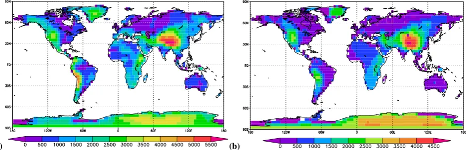
The parameterization of the subgrid-scale orography of ECHAM5 is adjusted to ensure consistency with the modi-fied mid-Pliocene elevation. For the PI setup of ECHAM5, the input parameters for the parameterization scheme have been retrieved using algorithms that rely on a highly resolved topography (see Sect. 3.1), which in general is not available from elevation reconstructions. We therefore interpolate the mid-Pliocene elevation of the atmosphere model to a higher resolution (0.5◦×0.5◦) prior to calculation of the subgrid-scale orography parameters. In Fig. 2 we show an examplary comparison of the hereby generated mid-Pliocene orographic peaks elevation to its PI counterpart. It is inevitable that the precision of the subgrid-scale orography parameterization is lower in the mid-Pliocene setup than in the PI setup.

As a boundary condition for the land-based mid-Pliocene cryosphere, we extract the ice sheet distribution from the vegetation reconstruction (file biome veg v1.3.nc, Salzmann et al., 2008a,b; Hill et al., 2007) and interpolate it to T31-resolution. To generate the mid-Pliocene SST forc-ing for experiment 1, we subtract from the monthly mid-Pliocene SST reconstruction (file PRISM3 SST v1.1.nc, Dowsett, 2007; Robinson et al., 2008; Dowsett and Robin-son, 2009; Dowsett et al., 2009) the modern SST distribution (file PRISM3 modern SST.nc), interpolate the resulting mid-Pliocene SST anomaly to T31-resolution (Fig. 3), and add it to the standard PI SST forcing of ECHAM5. At locations where the mid-Pliocene temperature reconstruction does not match to the ECHAM5 land-sea mask, the SST reconstruc-tion is extrapolated.

Mid-Pliocene sea ice forcing is generated considering the PRISM3 mid-Pliocene SST anomaly in T31-resolution and the PI ECHAM5 sea ice distribution. Our method assumes that at any location a warming of the PI ocean surface will fully remove the sea ice cover. We determine the sign of the mid-Pliocene SST anomaly, and at locations where this sign is positive we remove sea ice from the monthly PI sea ice forcing. By this method we retrieve a mid-Pliocene sea ice distribution that is consistent with the SST forcing. The mid-Pliocene Arctic Ocean is nearly ice-free in summer, maxi-mum sea ice cover is found in January (Fig. 3).

(6)

(a) 180˚ 180˚

240˚ 240˚

300˚ 300˚

0˚ 0˚

60˚ 60˚

120˚ 120˚

180˚ 180˚

−90˚ −90˚

−60˚ −60˚

−30˚ −30˚

0˚ 0˚

30˚ 30˚

60˚ 60˚

90˚ 90˚

(b) 180˚

180˚

240˚ 240˚

300˚ 300˚

0˚ 0˚

60˚ 60˚

120˚ 120˚

180˚ 180˚

−90˚ −90˚

−60˚ −60˚

−30˚ −30˚

0˚ 0˚

30˚ 30˚

60˚ 60˚

90˚ 90˚

Fig. 1. Land-sea distribution on the ocean model grid as used in the PMIP3 PI control simulation (a) and the PlioMIP mid-Pliocene simulation (b) of experiment 2. There are two grid poles (white areas) which are located over Greenland and Antarctica. The nominal grid resolution

of 3◦×1.8◦of the 122×101 grid varies; it is high in polar regions and highest around Greenland. Both land-sea distributions are identical

with the exception of the closure of the Hudson Bay and modifications in the West Antarctic in the case of the mid-Pliocene experiment. For clarity, only every second grid line is shown in the graph.

(a) (b)

Fig. 2. Comparison of the orographic peaks elevation in units of m as used in the PI control simulation (a) to its mid-Pliocene counterpart (b), which has been generated from a coarse mid-Pliocene topography.

anomalies and the PI temperature state of the MPI-OM model to 1◦×1◦ and 33 layers, and a subsequent interpo-lation to the GR30/L40 grid.

In the mid-Pliocene simulation of experiment 2, the HD-model is adjusted to the modified topography. This facilitates that the hydrological cycle is closed, and that runoff to the ocean is simulated realistically. The mid-Pliocene 0.5◦×0.5◦ elevation of the HD-model is generated using a topogra-phy anomaly procedure that is similar to the one applied for ECHAM5 as described above, i.e. by adding the 0.5◦×0.5◦ interpolated mid-Pliocene elevation anomaly to the PI eleva-tion of the HD-model. The high-resolueleva-tion glacier mask is generated by 0.5◦_×₀_.₅◦_{interpolation of the land ice}

recon-struction. The land-sea mask is taken from the HD-model’s PI setup, and the Hudson Bay is closed manually. Mid-Pliocene land-sea mask, elevation and glacier mask of the HD-model are used to calculate additional parameters. In Fig. 4a and b we show as an example the river direction data sets of the PI control and mid-Pliocene setup.

According to the PlioMIP protocol, a fixed vegetation re-construction has to be prescribed for mid-Pliocene simula-tions. In order to pin JSBACH to the vegetation reconstruc-tion, its dynamic vegetation module is disabled. The stan-dard PI vegetation is replaced by the mid-Pliocene vegetation reconstruction. Unfortunately, the treatment of vegetation in JSBACH is not directly comparable to the information pro-vided by the PRISM3 reconstruction data set. Generation of the mid-Pliocene vegetation forcing therefore is performed in a two-step approach. First, we apply a calibration method to transform each PRISM3 biome into a form that is compat-ible to JSBACH. Second, we use this information to produce the global mid-Pliocene vegetation forcing for JSBACH.

(7)

(a) (b)

Fig. 3. Anomaly between the climatological SST forcings of the mid-Pliocene and PI control simulations of experiment 1 in units of◦C. The

green contours indicate the 90 % isoline of the absolute sea ice cover prescribed for the mid-Pliocene simulation. Shown are the forcings for the months January (a) and August (b).

(a) (b)

Fig. 4. River directions on the hydrological model grid (0.5◦×0.5◦) of ECHAM5 for PI control (a) and adjusted to Pliocene topography (b).

The colours indicate the flow direction at each grid point; ocean is indicated by white. In addition to the four main and diagonal directions, dark blue (O) marks grid cells where the water flow is directly into the ocean (coastal gridpoints).

fraction of a grid cell; the second parameter provides infor-mation on the relative abundance of each PFT. For each grid cell of the land surface, the first parameter is a single rational number with a value in the range[0,1]. Since at every grid cell in principle several or even all of the eight PFTs may be present, the second parameter consists of a set of eight rational numbers in the range[0,1]that add up to 1.

The calibration procedure relies on the assumption that modern observed biome distribution and PI control JSBACH vegetation cover are compatible and represent similar in-formation. We generate global masks in T31-resolution that identify locations where a specific observed modern biome (file BAS Observ BIOME.nc) is present. These bi-nary masks are multiplied to a 50-yr average PI vegetation cover as simulated by JSBACH (Wei et al., 2012). The inten-tion is to retrieve a JSBACH vegetainten-tion distribuinten-tion that cor-responds to a specific biome. These vegetation distributions, consisting of relative PFT abundances and vegetation

densi-ties for all locations that coincide with the location of a spe-cific biome, are then averaged to retrieve a typical PFT com-bination and vegetation density that represents this biome.

This biome representation is used in a second step to cre-ate the mid-Pliocene vegetation forcing: We interpolcre-ate the PRISM3 vegetation reconstruction (file biome veg v1.3.nc, Salzmann et al., 2008a,b; Hill et al., 2007) to T31-resolution, and replace every biome by the corresponding PFT combina-tion and vegetacombina-tion density. Land areas in our mid-Pliocene setup, which have no counterpart in the vegetation recon-struction due to small inconsistencies between the land-sea masks, are forced with vegetation parameters of a nearby lo-cation.

(8)

(a)

Fig. 7. Vegetation forcing for PI control and Pliocene: Forest fractions for PI(a)and mid-Pliocene(b), grass fractions for PI(c)and mid-Pliocene(d). See text for details.

33

(b)

33

(c)

33

(d)

33

Fig. 5. Vegetation forcing for PI control and Pliocene: Forest fractions for PI (a) and Pliocene (b), grass fractions for PI (c) and mid-Pliocene (d). See text for details.

(a) gl ob al a vg . 2 m -t em p er at u re / °C 12 13 14 15 16 17 18

experiment simulation time / model year 0 2 4 6 8

experiment 1 mid-Pliocene experiment 1 PI control model time axis / year

800 810 820 830 840 850

experiment simulation time / model year

0 10 20 30 40 50

an n u al m ea n o f gl ob al a ve ra ge 2 m -t em p er at u re / °C 14.5 15.0 15.5 16.0 16.5 (b)

potential temperature @700 m potential temperature @2200 m salinity @700 m

salinity @2200 m model time axis / year

800 1000 1200 1400 1600

mid-Pliocene experiment simulation time / model year

0 200 400 600 800 1000

sa li n it y / p su 35.0 35.2 35.5 35.8 p ot en ti al t em p er at u re / °C 6.0 7.0 8.0 9.0 10.0 11.0 12.0

Fig. 6. (a) Evolution of yearly average 2-m temperature in experiment 1. The atmosphere adjusts to the change in climate forcing very fast (cf. the inset that shows a monthly resolved time series of the first 10 simulation years), and reaches an equilibrium state in less than ten years. (b) Annual mean North Atlantic Ocean temperature and salinity at 700 m and 2200 m in the mid-Pliocene simulation of experiment 2. Starting point of the simulation is a temperature-adjusted PI control state at year 800 of the model time axis (see text for details). Output between model years 600 and 749 is missing, as indicated by the straight progression of the graph.

grass fractions are calculated for each grid cell by summing over the relative abundances of the contributing PFTs in the JSBACH vegetation forcing and weighing this value by the vegetation density. The forest fraction incorporates JSBACH PFTs 1, 2, 3 and 4, which comprise different types of

for-est. The grass fraction includes shrubs, tundra, C3 and C4 grasses, i.e. JSBACH PFTs 5, 6, 7 and 8 (Table 1).

(9)

(a)

experiment 1 PI control experiment 1 mid-Pliocene experiment 1 anomaly experiment 2 PI control experiment 2 mid-Pliocene experiment 2 anomaly

latitude / °N

−75 −50 −25 0 25 50 75

zo n al a ve ra ge t em p er at u re a n om al y (l an d ) / ° C -20.0 -15.0 -10.0 -5.0 0.0 5.0 10.0 15.0 zo n al a ve ra ge t em p er at u re ( la n d ) / ° C -40.0 -30.0 -20.0 -10.0 0.0 10.0 20.0 30.0 (b) zo n al a ve ra ge t em p er at u re a n om al y (o ce an ) / ° C -10.0 -5.0 0.0 5.0 10.0 15.0

latitude / °N

−75 −50 −25 0 25 50 75

zo n al a ve ra ge t em p er at u re ( oc ea n ) / ° C -20.0 -10.0 0.0 10.0 20.0 30.0 (c)

zo n al a ve ra ge t em p er at u re a n om al y (l an d a n d o ce an ) / ° C -20.0 -15.0 -10.0 -5.0 0.0 5.0 10.0 15.0

latitude / °N

−75 −50 −25 0 25 50 75

zo n al a ve ra ge t em p er at u re ( la n d a n d o ce an ) / ° C -40.0 -30.0 -20.0 -10.0 0.0 10.0 20.0 30.0 (d)

latitude / °N

−75 −50 −25 0 25 50 75

zo n al a ve ra ge p re ci p it at io n a n om al y (l an d a n d o ce an ) / m m d -1 -2.0 0.0 2.0 4.0 6.0 8.0 10.0 zo n al a ve ra ge p re ci p it at io n ( la n d a n d o ce an ) / m m d -1 -2.0 0.0 2.0 4.0 6.0 8.0 10.0

Fig. 7. Zonal averages and average anomalies of SAT in◦C for land areas (a), oceans (b), and land and ocean (c). Shown are absolute values

for the PI control and mid-Pliocene simulations of experiments 1 and 2, as well as the respective anomalies. Zonal averages and average anomalies of precipitation for land and ocean (d). All values have been retrieved from a 30-yr climatology.

at the expense of the density of grass cover. On Green-land, both forest and grass vegetation are introduced as a result of the reduction of the prescribed ice sheet. The loss of ice cover on Antarctica is balanced by the emergence of a grass-dominated vegetation. Grasslands are expand-ing over Europe, where forest becomes rarer. In northern Africa, both grass and forest cover are expanding towards the Mediterranean Sea, grass being the dominant vegetation cover around the area of the present-day Sahara. In the south-ern part of Africa and the northsouth-ern part of South America, forest cover decreases while the grass cover becomes more dense. On the Australian continent, a displacement of the grass cover toward the south-west is evident, opposed by a north-eastward shift of the forest cover. In summary, the veg-etation forcing for the mid-Pliocene simulation exhibits more grass cover than the PI control simulation, with the obvious

exception of the continental northern high latitudes, where forest becomes more abundant.

Orbital forcing and concentrations of trace gases in the mid-Pliocene simulations are identical to the PI control setup with the exception of carbon dioxide. Its concentration has been changed to a uniform and constant volume mixing ratio of 405 ppm as requested by the PlioMIP protocol. This value is in the range of paleo-reconstructions of carbon dioxide, suggesting values between 360 ppm (K¨urschner et al., 1996) and 425 ppm (Raymo et al., 1996) for the Pliocene.

(10)

(a)

Fig. 10. Anomalies of SAT in◦Cbetween the mid-Pliocene and PI control runs of experiment 1. Shown are annual mean(a), boreal winter season (DJF)(b), and boreal summer season (JJA)(c)retrieved from a30 y

climatology.

36

(b)

Fig. 10. Anomalies of SAT in◦Cbetween the mid-Pliocene and PI control runs of experiment 1. Shown are annual mean(a), boreal winter season (DJF)(b), and boreal summer season (JJA)(c) retrieved from a30 y

climatology.

36

(c)

Fig. 10. Anomalies of SAT in◦Cbetween the mid-Pliocene and PI control runs of experiment 1. Shown are annual mean (a), boreal winter season (DJF)(b), and boreal summer season (JJA)(c)retrieved from a30 y

climatology.

36

Fig. 8. Anomalies of SAT in◦C between the mid-Pliocene and PI control runs of experiment 1. Shown are annual mean (a), boreal winter

season (DJF) (b), and boreal summer season (JJA) (c), retrieved from a 30-yr climatology. Strong temperature anomalies over the Hudson Bay are caused by the change in the land-sea mask.

PlioMIP project are retrieved by calculating the multi-year monthly average over the last 30 yr of the simulations.

Simulations of experiment 2 are integrated for ≈1000 model years; the last 30 yr of the time integration are used for the calculation of experimental climatologies for the PlioMIP project. The initial ocean state for the PI control simulation is retrieved from a spin-up generated for the Millenium Ex-periment (Jungclaus et al., 2010), which has been integrated further for about 3000 yr in a standalone ocean simulation. Preparation of the initial ocean state for the mid-Pliocene simulation is described in Sect. 3.2. At the end of the mid-Pliocene simulation, the upper ocean is nearly in an equi-librium state, both with respect to temperature and salinity distribution. On the other hand, the deep ocean at 2200 m still shows a drift (Fig. 6b). This suggests that the deep ocean in our mid-Pliocene simulation is not completely adjusted to the model forcing. Previous paleoclimatic simulations with COSMOS show that, in the given model configuration, the deep ocean requires a simulation time of the order of 5000 yr for complete relaxation. Such long-term integrations are not feasible within the framework of our contribution to PlioMIP.

4 Results

In this section we present general results of our PI and mid-Pliocene simulations of PlioMIP experiments 1 and 2. We first give an overview of a selection of global and zonal aver-age climatological parameters of the simulations, and present subsequently in more detail anomalies that result from the implementation of mid-Pliocene boundary conditions into our climate model.

(11)

(a)

Fig. 11.As Fig. 10, but for experiment 2 where we have used the coupled atmosphere-ocean circulation model.

37

(b)

37

(c)

37

Fig. 9. As Fig. 8, but for experiment 2 where we have used the coupled atmosphere-ocean circulation model.

Table 2. Major annual globally averaged climatological parameters of PI control and mid-Pliocene standalone atmosphere (A) and coupled atmosphere-ocean (AO) simulations for the last 30 model years of simulations: The TOA global energy imbalance has been calculated by averaging the sum of TOA downward shortwave radiation, TOA upward shortwave radiation, and TOA upward longwave radiation. Globally averaged SATs are given for the PI control and mid-Pliocene simulations of experiments 1 and 2 as absolute values. For the mid-Pliocene

simulations, the anomaly1T with respect to the corresponding control simulation is given in brackets. Global average precipitation is given

in units of kg m−2s−1(the internal unit in ECHAM5) and converted to mm d−1.

simulation (A/AO) TOA imbalance/ SAT (1T)/ precipitation/

W m−2 ◦C kg m−2s−1(mm d−1)

PI control experiment 1 (A) −0.36 15.12 3.28×10−5(2.83)

mid-Pliocene experiment 1 (A) 3.50 17.35 (2.23) 3.39×10−5(2.93)

PI control experiment 2 (AO) 1.72 14.42 3.15×10−5(2.72)

mid-Pliocene experiment 2 (AO) 1.61 17.82 (3.40) 3.37×10−5(2.91)

appears to be slightly farther from radiative equilibrium with a persisting net energy imbalance of 3.5 W m−2, while the PI control simulation shows a small TOA net energy imbalance of≈0.4 W m−2. Since the atmosphere is well-equilibrated during the last 30 yr of experiment 1 (Fig. 6a), net energy fluxes are unlikely to be caused by remaining energy buffers in the model climate (like the deep ocean in experiment 2), but are presumably caused by inconsistencies in the pre-scribed SST field. The signs of the residual energy fluxes suggest that the prescribed SST is slightly too warm (too

cold) in the PI control (mid-Pliocene) simulation of exper-iment 1 with respect to radiative equilibrium in ECHAM5. For the PI simulation, this conclusion is supported by Fig. 7b where zonal average ocean surface air temperature (SAT) is plotted versus latitude. If one assumes that the PI simulation of experiment 2 is close to radiative equilibrium, then it is evident that, in many regions of the mid- and high latitudes, the prescribed PI SST of experiment 1 is too warm.

(12)

(a)

Fig. 12. Anomalies of precipitation inmm d−1 between the mid-Pliocene and PI control runs of experiment 1. Shown are annual mean (a), boreal winter season (DJF)(b), and boreal summer season (JJA) (c). Time averages have been calculated from a30 yclimatology.

38

(b)

Fig. 12. Anomalies of precipitation inmm d−1 between the mid-Pliocene and PI control runs of experiment 1. Shown are annual mean(a), boreal winter season (DJF)(b), and boreal summer season (JJA)(c). Time averages have been calculated from a30 yclimatology.

38

(c)

Fig. 12. Anomalies of precipitation inmm d−1 between the mid-Pliocene and PI control runs of experiment 1. Shown are annual mean(a), boreal winter season (DJF) (b), and boreal summer season (JJA)(c). Time averages have been calculated from a30 yclimatology.

38

Fig. 10. Anomalies of precipitation in mm d−1between the mid-Pliocene and PI control runs of experiment 1. Shown are annual mean (a),

boreal winter season (DJF) (b), and boreal summer season (JJA) (c). Time averages have been calculated from a 30-yr climatology.

in experiment 2. Annual globally averaged surface air temperatures T of the PI control simulations of experi-ment 1 and 2 are T=15.12◦C andT =14.42◦C, respec-tively. Jones et al. (1999) estimate from a global SAT database T=14.0◦C for the period from 1961–1990. Our PI control climate therefore seems to be comparably warm. Since we are mainly interested in analysing the differences between PI and mid-Pliocene simulations, we do not con-sider the potential deviation of our PI climate from an ideal reconstructed PI climatology to be of relevance for this study. The mid-Pliocene simulations generally are warmer and wetter than the respective PI control simulations. Warm-ing and intensification of precipitation are stronger in the coupled atmosphere-ocean setup of experiment 2. Here, we find 1T=3.40◦C and 1P =0.19 mm d−1, compared to 1T=2.23◦C and1P =0.10 mm d−1in experiment 1. The amplitude of 1T that we observe in both experiments is in agreement with results documented in other publications, which suggest a mid-Pliocene global temperature anomaly of about 2◦C – 3◦C with respect to PI (e.g. Jansen et al., 2007). The warming observed in our simulations exhibits a strong latitudinal dependency. The zonally averaged SAT anomaly over land is below 1T=5◦C in low and

(13)

(a)

Fig. 13.As Fig. 12, but for experiment 2.

39

(b)

39

(c)

39

Fig. 11. As Fig. 10, but for experiment 2.

comparably low temperatures at low latitudes, which in the standalone atmosphere simulation are present due to the pre-scribed mid-Pliocene temperature reconstruction (Dowsett, 2007; Robinson et al., 2008; Dowsett and Robinson, 2009; Dowsett et al., 2009).

The hydrological cycle is enhanced in our mid-Pliocene simulations, especially in high latitudes. In both experiments we find increased precipitation poleward of 50◦N and 50◦S, which especially in experiment 2 is at the expense of precip-itation in the subtropics at around 30◦N and 30◦S (Fig. 7d). The sign of anomalous tropical precipitation differs between experiments 1 and 2: In experiment 2 rainfall increases, es-pecially north of the Equator by about 1 mm d−1. In experi-ment 1 equatorial precipitation weakens.

4.2 Spatially and seasonally resolved mid-Pliocene anomalies of atmospheric quantities

A seasonally resolved consideration of global SAT anomaly maps for experiment 1 (Fig. 8) and experiment 2 (Fig. 9) al-lows us to identify regions and seasons where temperature is affected strongest by the implementation of mid-Pliocene forcing. The most pronounced annual average warming oc-curs in polar regions (Fig. 8a, 9a), especially over areas where strong changes of albedo and orography have been

im-plemented, i.e. over Greenland and Antarctica. Over Green-land the warming due to the topographic effect seems to be the major driver for mid-Pliocene warmth. For a typical location over Greenland, which is free of ice in the mid-Pliocene simulation of experiment 2, we find a warming of ≈15◦C with respect to PI. The mid-Pliocene elevation at this location is decreased by≈1800 m. Therefore, about 80 % of the warming is related to elevation reduction if one assumes a lapse rate of 6.5 K/1000 m. High-latitude warm-ing is strongest in the respective local winter season (DJF (JJA) for the Northern (Southern) Hemisphere, Fig. 8b, 8c, 9b, 9c). In the Northern Hemisphere, temperature anoma-lies are most pronounced in experiment 2, where tempera-ture anomalies of more than 10◦_{C extend over North}

Amer-ica and Eurasia. Over the Eurasian landmass, the pronounced warming crosses 60◦_{N in the center of the continent.}

(14)

(a) (b)

(c)

Fig. 12. Annual mean SST in◦C in experiment 2 for the PI control simulation (a), the mid-Pliocene simulation (b), and the anomaly between

mid-Pliocene and PI control (c). The expansion of the equatorial warm pool is indicated by the bold grey 28.5◦C isoline (a, b). In addition

to the SST fields, we show in (a, b) thin green isolines depicting the absolute values of fractional sea ice cover. The contour interval is 0.15.

The percentage of PI sea ice cover that is still available at a specific location in the mid-Pliocene simulation is indicated by thin green isolines

in (c). The contour interval is 0.15. All values represent time averages calculated from a 30-yr climatology that has been interpolated to a

regular 360◦×180◦grid.

is absent in the temperature reconstruction, is simulated in the northern North Pacific Ocean. In general, regions where a slight cooling or a moderate warming of less than 2◦C is observed in experiment 1 are less common in experiment 2. This is evident over large parts of the ocean between 60◦S and 30◦N, and over land in the Rocky Mountains, the north-ern Andes, over Africa, the Tibetan Plateau and Australia.

Spatially resolved anomalies of precipitation (i.e. the sum over convective and large-scale rainfall) are shown in Fig. 10 and 11. We consider anomalies of the annual mean (Fig. 10a, 11a), boreal winter (DJF, Fig. 10b, 11b), and boreal sum-mer (JJA, Fig. 10c, 11c). The high-latitude trend towards in-creased precipitation observed in the precipitation profiles of the mid-Pliocene simulations (Fig. 7d) is evident in the sum-mer and winter seasons and the annual mean. Over North America we find a dipole of increased precipitation in the Rocky Mountains and reduced rain in the east of the land-mass. This dipole structure is strongest in the winter season, and more pronounced if SST is prescribed. South America receives less precipitation on average, but local summer

rain-fall increases in the northern part of the continent. Drying of the Tibetan Plateau occurs in particular in experiment 2. Precipitation over the equatorial eastern Pacific Ocean, the Atlantic Ocean, and the Indian Ocean shifts northward. This effect is most pronounced in experiment 2 and explains the strong increase in rainfall north of the Equator as depicted in Fig. 7d. The decrease in tropical precipitation, observed in experiment 1, is mainly located over the equatorial Atlantic Ocean, the Pacific Ocean, and especially the Indian Ocean.

(15)

(a) (b)

(c)

Fig. 13. Annual mean sea surface salinity in psu in experiment 2, calculated from a 30-yr climatology that has been interpolated to a regular

360◦×180◦grid. Shown are the PI control simulation (a), the mid-Pliocene simulation (b), as well as the anomaly between mid-Pliocene

and PI control (c).

(a) (b)

Fig. 14. AMOC in Sv for PI control (a) and mid-Pliocene (b) simulations of experiment 2. Overturning rates are time averages that have been calculated from 30-yr climatologies. Positive values represent a clockwise circulation, contour line interval is 1.5 Sv. The grey area indicates bottom topography calculated from the basin-wide zonal minimum sea floor elevation.

Pacific Ocean, while precipitation increases at the Equator. Under the influence of the mid-Pliocene SST reconstruction in experiment 1, the dominant anomaly pattern is an increase

(16)

(a) (b)

Fig. 15. As Fig. 14, but for the GMOC. Contour line interval is 2 Sv.

(a) (b)

Fig. 16. As Fig. 14, but for the PMOC. Contour line interval is 1.5 Sv.

the boreal summer season. In the fully coupled simulation of experiment 2, a general drying is observed at this location. This hints to differences in the behaviour of the mid-Pliocene monsoon between experiments 1 and 2.

4.3 Mid-Pliocene anomalies of oceanic quantities

In the coupled atmosphere-ocean simulation of experiment 2, the sea surface can evolve freely according to the physics of the climate model. As a result, the SST of the coupled mid-Pliocene simulation does not necessarily follow the re-construction, which is clearly the case in our simulations as previously discussed. Global maps of absolute SST of the PI control and Pliocene simulation show that in the mid-Pliocene the equatorial warm pools of the Atlantic Ocean, the Pacific Ocean, and the Indian Ocean have increased max-imum temperatures and extents (compare Fig. 12a and 12b).

Such a low-latitude warming is not supported by the recon-struction (see Fig. 3). A plot of temperature anomalies be-tween mid-Pliocene and PI control confirms observations of SAT that have been described above: In the Indian Ocean sector of the Southern Ocean, a warming of more than 3◦_C

is apparent. A substantial ocean surface warming occurs also in the North Atlantic Ocean and extends into the Norwegian Sea and the Barents Sea (Fig. 12c). The Pacific Ocean warms especially in northern and western regions. Warming of the North Atlantic Ocean and adjoint regions is supported by the SST reconstruction, but comparably weak in our simulation. In the eastern Pacific Ocean, the warming is also smaller than expected. The simulated temperature increase in the North Pacific Ocean, on the other hand, seems to be stronger than reconstructed.

(17)

Ocean sector of the Southern Ocean, the Weddell Sea, the In-dian Sector of the Pacific Ocean, the Barents Sea, Kara Sea, Bering Sea, Chukchi Sea, and the Beaufort Sea, a substan-tial loss of ice cover is evident (compare Fig. 12a and 12b). In the Pacific Ocean sector of the Southern Ocean, the posi-tion of the sea ice border is rather unchanged, but the density of sea ice is decreased. Large areas of the Arctic Ocean are still covered by sea ice, but its density is also substantially decreased with respect to the PI control simulation.

Ocean surface salinity in the PI control simulation is char-acterized by high concentrations in the Atlantic Ocean, es-pecially in the mid-latitude evaporation regions, the Mediter-ranean Sea and the Red Sea. The Baltic Sea, the Hudson Bay, the North Pacific Ocean and the Arctic Ocean are compa-rably fresh. These general oceanographic patterns are also found in the mid-Pliocene simulation (compare Fig. 13a and 13b), but the contrast between high and low saline regions intensifies (Fig. 13c): Salinity increases in the Mediterranean Sea and the Atlantic Ocean, while the Arctic Ocean and large parts of the Pacific Ocean freshen. An exception to this rule are regions in the western North Pacific Ocean, where salin-ity increases at an amplitude that is comparable to patterns found in the Atlantic Ocean.

In the mid-Pliocene Atlantic Ocean, inflow of deep water from the South Atlantic Ocean is decreased, but the merid-ional overturning circulation of the upper branch is slightly enhanced (compare Fig. 14a and 14b). The maximum of meridional volume transport extends, while the general struc-ture of the Atlantic Ocean meridional overturning circulation (AMOC) is comparable to the PI control run. The globally integrated overturning circulation (GMOC) is more vigorous in the upper branch of the meridional flow regime of the mid-Pliocene simulation, while the lower branch is nearly in an off-mode (compare Fig. 15a and 15b). North of 20◦N we calculate the Pacific Ocean meridional overturning circula-tion (PMOC), which is not a standard output of COSMOS, by subtracting AMOC from GMOC. We observe that in the mid-Pliocene there is a small formation of intermediate water in the mid-latitude Pacific Ocean between 40◦N and 60◦N that is not present in the PI control simulation (compare Fig. 16a and 16b).

5 Discussion

In this section we first discuss some aspects of the exper-imental methodology described in Sect. 3. The discussion concludes with an evaluation of some of the results presented in Sect. 4.

5.1 Experimental methodology

The radiative forcing of experiment 2 differs slightly from the PlioMIP experimental protocol with respect to the value of the solar constant. As described above, the solar constant

in our version of the ECHAM5 model is a fixed parameter. In standalone mode its value is set to 1365 W m−2_{; if coupled} to an ocean model, it is slightly higher (1367 W m−2_{). Since} all other paleoclimate simulations conducted in COSMOS rely on these standard ECHAM5 parameters, we also pre-serve them in the PlioMIP simulations. To estimate the effect of the difference in the solar constant, we set up a modified standalone atmosphere mid-Pliocene simulation with an in-creased solar constant (1367 W m−2). All other settings are identical to our mid-Pliocene simulation of experiment 1. The anomaly of SAT between the simulation with high and low solar constant is by construction negligible over the ocean. Over land the change in SAT is not vanishing, but the time-averaged anomalies of global meanT andP intro-duced by the change in the solar constant are again negli-gible: The values ofT andP of both mid-Pliocene simula-tions are identical if rounded to the second decimal place. We therefore conclude that the general global average climatol-ogy of experiment 1 is not influenced appreciably by a small modification of the solar constant by 2 W m−2. Therefore, our climatology of PlioMIP experiment 1 with 1365 W m−2 is comparable to one that we would have retrieved with a solar constant of 1367 W m−2, and hence our experiments 1 and 2 are comparable.

In the PRISM3 topographic boundary condition of the mid-Pliocene, a global sea level rise of 25 m due to warm-ing and the related reduction of land ice volume is prescribed (Haywood et al., 2010). Adjusting the land-sea mask of the ocean model to this change involves an interpolation rou-tine, which leads to strong and undesired alterations of the continental borders and gateways. In the mid-Pliocene simu-lations of our experiments, we therefore neglect the change in land-sea distribution resulting from a global sea-level rise, and preserve the PI land-sea mask of both the atmosphere and ocean models. Exceptions are the manual closure of the Hud-son Bay and small modifications at the West Antarctic. The small removal of land in the ocean model at the West Antarc-tic cannot be adequately reproduced on the non-fractional land-sea mask of the atmosphere model. Therefore, at this lo-cation minor inconsistencies in the exchange of momentum, heat and freshwater may arise. This is a general problem of models with a non-fractional land-sea mask.

(18)

by calculating one typical value of PFT distribution and veg-etation density over a large area. This leads to a reduced spatial variability of vegetation in the mid-Pliocene simula-tions. We have tested the sensitivity of the PI control climate of experiment 1 to such a reduced spatial vegetation vari-ability (see Appendix). The global average SAT is not appre-ciably affected by the change in the prescribed vegetation. We therefore conclude that PI control and mid-Pliocene sim-ulations of experiments 1 and 2 are comparable, despite the flawed vegetation variability in the paleo-simulations. Never-theless, these facts should be kept in mind when comparing results taken from our simulations to those of other groups, who have possibly devised different methods for implement-ing the vegetation reconstruction into their simulations.

For experiment 2, there is an additional difference between the methodologies of the PI control run (that is identical to the PMIP3 PI control run) and the mid-Pliocene simulation, since the PlioMIP protocol is specific in that the use of a fixed vegetation is requested. Therefore, the mid-Pliocene simula-tion of experiment 2 runs with a fixed vegetasimula-tion distribusimula-tion, while the vegetation of the PI control simulation is equili-brated and stable, but in principle might change over time due to the use of the dynamic vegetation module. As a re-sult, the variability of the vegetation cover of both simula-tions may differ on a temporal scale. We tested the impact of this different methodology in an additional sensitivity study in which parts of the equilibrated PI control simulation were conducted again without the use of the dynamic vegetation module. We calculated and compared the average and stan-dard deviation of global mean SAT over 50-yr intervals that only differ with respect to the use of the dynamic vegetation module. The change in global average SAT between intervals simulated with fixed vegetation, and intervals in which the vegetation was equilibrated but not fixed, is within one stan-dard deviation. Furthermore, the stanstan-dard deviation of global mean SAT does not change appreciably if the dynamic vege-tation module is switched off. We therefore conclude that the use of fixed vegetation only in the mid-Pliocene simulation of experiment 2 does not impede its comparability to the PI control run.

For the generation of the mid-Pliocene sea ice forcing of experiment 1, we relied on a procedure in which we re-moved the PI sea ice cover in the ECHAM5 forcing at lo-cations where the mid-Pliocene SST reconstruction reports a warming (see Sect. 3.2). This procedure is compatible with the generation of the mid-Pliocene SST forcing which re-lies on temperature anomare-lies. It assumes that warming in the mid-Pliocene is able to melt all the PI ice at a specific location. This assumption might be justified if an equilib-rium climate state is concerned, which certainly is the case for our model forcing fields. An alternative way of generat-ing a mid-Pliocene sea ice reconstruction could rely on the calculation of the lost ice volume under consideration of the amount of energy that is supplied by mid-Pliocene warming. Subtraction of the lost ice volume from the PI sea ice

forc-ing in principle might lead to a different mid-Pliocene sea ice cover at locations where PI sea ice is thick enough to partly survive the heat excess. Unfortunately, we do not have infor-mation on the thickness of the prescribed PI sea ice distribu-tion (which is a mask that lacks informadistribu-tion about the verti-cal dimension). As a first-order approximation, we therefore rely on the procedure which assumes an infinite energy sup-ply (or alternatively vanishing ice thickness). We also tested the equivalence of this approach to the alternative extraction of the sea ice cover directly from the mid-Pliocene temper-ature reconstruction (i.e. by assuming the presence of mid-Pliocene sea ice wherever the reconstructed SST is at the freezing point of sea water). The differences with respect to our approach are marginal.

5.2 Experimental results

When comparing the mid-Pliocene SAT anomalies of exper-iment 1 and 2 (Fig. 7, 8, 9), we observe for ocean areas in experiment 2 the lack of specific patterns that are present in experiment 1. Since experiment 1 is forced with the SST re-construction, and since local SST and SAT are closely cou-pled in ice-free regions, we can conclude that differences in SAT anomaly patterns between both experiments identify re-gions where our coupled atmosphere-ocean setup is not able to reproduce the mid-Pliocene oceanography as it is inter-preted from the geological record. Obvious examples are the North Atlantic Ocean, the southeastern Pacific Ocean, and the equatorial regions: Our experiment 2 lacks the extreme warmth in the northern North Atlantic Ocean and the Nordic Seas, simulates too low temperatures in the southeastern Pa-cific Ocean, and is generally too warm in the tropics. In prin-ciple, the mid-Pliocene simulation of experiment 2 is char-acterized by a lower-than-PI meridional temperature range. However, we cannot reproduce the low mid-Pliocene SAT gradient suggested by the mid-Pliocene SST reconstruction that is inherent in experiment 1 (Dowsett, 2007; Robinson et al., 2008; Dowsett and Robinson, 2009; Dowsett et al., 2009, see Fig. 7b). The difference between the meridional temperature ranges of both simulations is about 5◦C. We therefore summarize that our experiment 2 does not repro-duce a number of ocean temperature patterns that are consid-ered to be critical features of the mid-Pliocene reconstruction (see e.g. Robinson (2009) for a discussion with respect to ex-treme warmth in the Arctic Ocean).

A model result, in which the mid-Pliocene simulations of both experiments agree, is the positive precipitation anomaly in high latitudes, as evident from Fig. 7d. The zonal aver-age increase in rainfall is most prominent in the Northern Hemisphere, where it amounts to approximately 0.5 mm d−1 – 1.0 mm d−1. The larger part of the excess precipitation is directly lost to the North Atlantic Ocean, but in both the local summer and winter seasons of experiments 1 and 2 (Fig. 10, 11) a certain amount (≈1 mm d−1 in experiment 2, up to

(19)

south-east of Greenland. In our mid-Pliocene setup, Green-land is therefore both wetter and warmer than the corre-sponding PI control simulations. The potential implications for the state and dynamics of the Greenland ice sheet, which has been prescribed in our simulations, pose an interesting question that will be addressed in a future study.

Our analysis of the meridional overturning circulation in the Atlantic Ocean and the Pacific Ocean shows that under mid-Pliocene conditions our climate model simulates a slight increase in the AMOC in the North Atlantic Ocean with re-spect to the maximum transport at 1000 m depth, while in-flow of deepwater from the South Atlantic Ocean is reduced. At the same time, we find formation of a small amount of intermediate water between 50◦N and 60◦N in the Pacific Ocean. It will be interesting to see whether these details of ocean circulation can be confirmed by other simulations in the framework of PlioMIP. The mechanisms behind the change in meridional volume transport, and the implications for the mid-Pliocene climate of the Northern Hemisphere, certainly deserve a deeper investigation which is beyond the scope of this manuscript.

6 Conclusions

We presented the layout of the PlioMIP simulations of ex-periments 1 and 2 that have been carried out at the Al-fred Wegener Institute in Germany, using the Earth system model COSMOS. Our model setup consists of the atmo-sphere model ECHAM5, the land surface and vegetation model JSBACH, and the ocean model MPI-OM. In the fully coupled atmosphere-ocean simulation of experiment 2, the low-latitude SST, which is influenced by the increased at-mospheric concentration of carbon dioxide, is overestimated with respect to experiment 1 and the proxy record. In par-ticular in the Northern Hemisphere, the meridional tem-perature range is larger in experiment 2. Our results sug-gest that the PI control and mid-Pliocene simulations are in (or close to) an equilibrium state, and that climatolo-gies of atmosphere quantities (e.g. SAT), and presumably of near-surface ocean quantities of the coupled atmosphere-ocean simulations, are stable. The TOA energy imbalance is small, i.e. about 1.6 W m−2in experiment 2. It is largest in the mid-Pliocene simulation of experiment 1 (3.5 W m−2). This shows that the energy balance in experiment 1 is not fully consistent with the prescribed SST and the atmosphere model. This is a common problem of uncoupled climate sce-narios.

Our setup of experiment 2 shows several aspects of mid-Pliocene oceanographic details when compared to the PRISM3 mid-Pliocene SST reconstruction (Dowsett, 2007; Robinson et al., 2008; Dowsett and Robinson, 2009; Dowsett et al., 2009), but there are obvious differences, e.g. with re-spect to tropical SST. In our Pliocene experiment 2, both the AMOC and PMOC are slightly enhanced contributing to an

increased northward heat transport. Another interesting fea-ture is the relatively fresh Pliocene Arctic Ocean and the more saline northern North Atlantic and Pacific Oceans. A deeper analysis of the mechanisms behind our model results, especially with respect to deviations from the proxy record, is beyond the scope of this study.

Despite problems with the reproduction of regional oceanographic features, we can in general reproduce a global mid-Pliocene climatology that is wetter and about 2◦C – 3◦C warmer than the PI control simulation, with a strong ampli-fication of warming in high latitudes. A comparison of our results to findings of other PlioMIP modelling groups, that includes derived quantities including climate sensitivity and Earth system sensitivity, is given by Haywood et al. (2012).

Appendix A

The influence of a smoothed vegetation on the PI control simulation

The approach of generating the mid-Pliocene vegetation forcing for JSBACH includes a translation of the modern observed vegetation distribution, which is given within the PlioMIP framework, into a PI vegetation distribution as sim-ulated with COSMOS. This leads to a smoothed vegeta-tion field, since the calculavegeta-tion of the fracvegeta-tional amount of a JSBACH PFT that corresponds to a specific biome of the modern observed vegetation is performed via averages over larger areas. The vegetation used in the PI simulations is not based on such a smoothed vegetation distribution with reduced spatial variability, since it is already available as a JSBACH vegetation field.

Here, we test the influence of reduced spatial vegetation variability in COSMOS (that is present in mid-Pliocene sim-ulations of experiments 1 and 2) on the resulting global cli-matology. To this end, we conduct the PI control simula-tion of experiment 1 again with a total integrasimula-tion time of 50 model years. The only change in the experimental setup is the use of the modern observed vegetation distribution to which we applied average vegetation properties as generated with the mapping procedure that is described in the article in Sect. 3.2, instead of using the long-term averaged PI vegeta-tion distribuvegeta-tion taken from COSMOS (that has been used in the PI control simulations of experiments 1 and 2). This veg-etation distribution therefore is comparable to PI simulations of experiments 1 and 2, but is smoothed as in the case of the mid-Pliocene simulations (Fig. A1).

(20)

(a) (b)

(c) (d)

Fig. A1. Comparison of the standard vegetation forcing, as used in the PlioMIP PI simulation of experiment 1, to a smoothed PI vegetation cover: Forest fractions for the standard (a) and smoothed (b) vegetation, and grass fractions for the standard (c) and smoothed (d) vegetation.

Fig. A2. Anomaly of SAT in◦C between a sensitivity study that

is forced with a smoothed PI vegetation, and the PI control run of experiment 1 with a PI vegetation that has not been subjected to smoothing. Shown is the annual mean retrieved from a 30-yr

clima-tology. The global average SAT anomaly is 0.02◦C.

are local anomalies of SAT especially over Asia and North America that are noteworthy (Fig. A2). We conclude that the global average climatology is not appreciably affected by the presence of a smoothed vegetation cover. The effect of a smoothed vegetation cover on regional temperatures is visible, but generally much smaller than the mid-Pliocene anomaly observed in experiments 1 and 2. Comparability of the PlioMIP mid-Pliocene and PI simulations is therefore not flawed by the presence of a smoothed vegetation cover in the mid-Pliocene simulations.

Acknowledgements. We would like to thank Ulrich Salzmann,

Reiner Schnur, Thomas Raddatz and Christian Reick for useful discussions on the implementation of the mid-Pliocene vegetation reconstruction into our simulations. We acknowledge the help from Stefan Hagemann with the preparation of the adjustments of the HD-model for the mid-Pliocene setup, and thank Xu Zhang for making available the model output that has been used to retrieve the PI control climatologies of experiment 2. Christian Stepanek’s work has been financed via a scholarship of the Helmholtz Graduate School for Polar and Marine Research (POLMAR). Gerrit Lohmann received funding through the Helmholtz research program PACES.