www.geosci-model-dev.net/7/1573/2014/ doi:10.5194/gmd-7-1573-2014
© Author(s) 2014. CC Attribution 3.0 License.
The generic MESSy submodel TENDENCY (v1.0) for process-based
analyses in Earth system models
R. Eichinger and P. Jöckel
Deutsches Zentrum für Luft- und Raumfahrt e.V. (DLR), Institut für Physik der Atmosphäre, Münchner Straße 20, Oberpfaffenhofen, 82234 Weßling, Germany
Correspondence to: R. Eichinger ([email protected])
Received: 20 February 2014 – Published in Geosci. Model Dev. Discuss.: 8 April 2014 Revised: 12 June 2014 – Accepted: 13 June 2014 – Published: 31 July 2014
Abstract. The tendencies of prognostic variables in Earth system models are usually only accessible, e.g. for output, as a sum over all physical, dynamical and chemical processes at the end of one time integration step. Information about the contribution of individual processes to the total tendency is lost, if no special precautions are implemented. The knowl-edge on individual contributions, however, can be of impor-tance to track down specific mechanisms in the model sys-tem. We present the new MESSy (Modular Earth Submodel System) infrastructure submodel TENDENCY and use it ex-emplarily within the EMAC (ECHAM/MESSy Atmospheric Chemistry) model to trace process-based tendencies of prog-nostic variables. The main idea is the outsourcing of the ten-dency accounting for the state variables from the process op-erators (submodels) to the TENDENCY submodel itself. In this way, a record of the tendencies of all process–prognostic variable pairs can be stored. The selection of these pairs can be specified by the user, tailor-made for the desired appli-cation, in order to minimise memory requirements. More-over, a standard interface allows the access to the individual process tendencies by other submodels, e.g. for on-line di-agnostics or for additional parameterisations, which depend on individual process tendencies. An optional closure test as-sures the correct treatment of tendency accounting in all sub-models and thus serves to reduce the model’s susceptibility. TENDENCY is independent of the time integration scheme and therefore the concept is applicable to other model sys-tems as well. Test simulations with TENDENCY show an increase of computing time for the EMAC model (in a setup without atmospheric chemistry) of 1.8±1 % due to the addi-tional subroutine calls when using TENDENCY. Exemplary results reveal the dissolving mechanisms of the stratospheric
tape recorder signal in height over time. The separation of the tendency of the specific humidity into the respective pro-cesses (large-scale clouds, convective clouds, large-scale ad-vection, vertical diffusion and methane oxidation) show that the upward propagating water vapour signal dissolves mainly because of the chemical and the advective contribution. The TENDENCY submodel is part of version 2.42 or later of MESSy.
1 Introduction
In Earth system models (ESMs) individual processes are de-scribed by various numerical algorithms for solving the un-derlying mathematical equations. Here, the term “process” describes any abstraction of a mechanism which alters the state of the system – these could be of physical, dynami-cal, chemidynami-cal, biogeochemidynami-cal, or even socio-economical na-ture. A corresponding “operator” describes the processes’ al-gorithmic formulation, which yields a deterministic output for any given (reasonable) input. Finally, within the Modular Earth Submodel System (MESSy) (Jöckel et al., 2005) we define any coded realisation of the corresponding operator as a “submodel”1. Thus, in a certain sense, the terms “process”, “operator” and “submodel” can be used as synonyms (and will be hereafter throughout the text).
The method of choice for the combination of the individual processes is the so-called operator splitting concept. In this 1Not all the MESSy submodels, however, necessarily represent
method the contributing processes modifying a specific prog-nostic variable are calculated in sequence, each adding its individual contribution to the overall change over time (i.e. the total tendency). Depending on the chosen time integra-tion scheme, these individual process tendencies (of a spe-cific prognostic variable) depend on the initial condition (or the state of the prognostic variable at the end of one or more time steps before), and the sum of the process tendencies at the same time step in the sequence of operators before. Commonly in ESMs only the total tendency is analysed and the information about the individual contribution of a cer-tain process to the change of a state variable is lost. Un-derstanding the effects of individual processes on the state variables, however, is important for unravelling the driving mechanisms of patterns generated by ESMs. Moreover, the process-based tendencies of state variables can serve as in-put to further calculations of physical or chemical processes. Approaching the issue by excerpting every process ten-dency of each state variable directly from the operators would cause a range of technical problems like an excessive memory usage and a very inflexible data handling. There-fore we implemented a comprehensive and easily expand-able infrastructure submodel, which is based on the out-sourcing of the tendency accounting from every process sub-model to it, and name it TENDENCY. Beginning with ver-sion 2.42 of MESSy (Jöckel et al., 2010) TENDENCY is part of the overall model infrastructure. TENDENCY operates on all prognostic variables, including tracers (generic sub-model TRACER, Jöckel et al., 2008). The structure of TEN-DENCY is independent of the time integration scheme used and thus the method is applicable to other model systems as well. Moreover, the process-based diagnostics can be set up by the user via namelist during runtime, tailor-made for the desired application, and thus avoiding a waste of mem-ory. In Sect. 2 the implementation of TENDENCY is de-scribed, including specifics of the used EMAC model sys-tem (Jöckel et al., 2010). The benefits and the methods of the user-controlled diagnostics are described in Sect. 3. Further-more, an optional closure test is explained, which is included in the TENDENCY submodel and makes the model less er-ror prone. A runtime performance analysis was carried out to determine the additional computing time arising from the increased usage of subroutine calls. Section 4 describes the test method and the results which indicate an overhead of 1.8±1 %. Exemplary results of the method are presented in Sect. 5.
A detailed reference manual of TENDENCY is available as a Supplement.
2 Implementation
ESMs aim to represent the physical and chemical processes of the real world as realistically and completely as possible. To approach this aim these processes are solved numerically
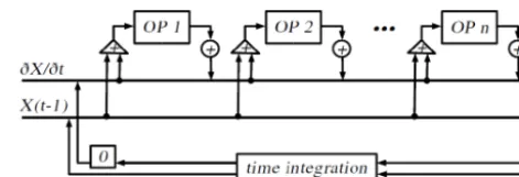
Figure 1. Operator splitting concept (image taken from Jöckel et al.,
2005). For explanation see text.
by individual algorithms. In the model the algorithms per-form sequentially as operators which alter the prognostic variables. The common method of choice for the sequential combination of the operators is the operator splitting concept, which is illustrated in Fig. 1.
According to this principle a total tendency is computed for a given state variable (X in Fig. 1) by the different op-erators (OP 1 . . . OPnin Fig. 1) in sequence and the sum (∂X/∂t) is added at the end of the time step to the value from the beginning of the time step (X(t−1)). We explain exemplarily the operator sequence controlling the specific humidityq in EMAC. The first operator to be called is ad-vect (OP 1), which simulates the adad-vection of water vapour. As all the tendencies are set to zero at the beginning of the model time step, the advect tendency is based solely on the initial value (X(t−1)). The next operator, e.g. vdiff (repre-senting vertical diffusion), computes a tendency based on the initial value and the tendency calculated by the advect opera-tor. The operator OPn, which in our example is cloud, hence is based on the initial value and the sum of the tendencies of all the previous operators. At the end of each time step the sum of all the tendencies calculated by the individual sub-models results in the total change of the prognostic variable. The individual process tendencies, however, are commonly computed within the respective operators and afterwards not used any more. Thus these values are overwritten in the fol-lowing time step and hence the information is lost.
Each MESSy submodel comprises subroutines for the initialisation, the time integration and the finalising phase. The submodels are connected via standardised interfaces and are controlled by a central unit (generic submodel SWITCH/CONTROL) calling one after the other. During the initialisation phase, among other things, the memory is set up, while during the integration phase the actual develop-ment of the state variables in space and time is calculated. The memory in the EMAC model is managed via the MESSy submodel CHANNEL (Jöckel et al., 2010), which we also utilise for TENDENCY.
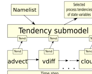
Commonly, within each prognostic submodel a process tendency for a specific state variable is calculated and added directly to the total tendency. The TENDENCY submodel is based on the outsourcing of this tendency accounting (i.e. the addition to the total tendency) from the submodels to the TENDENCY module. Figure 2 illustrates this concept. The addition of the process tendency to the total tendency in a specific submodel is replaced by a call to an interface sub-routine of TENDENCY, thus handing over the control over the tendency (Tend in Fig. 2). This allows us to keep a record of the process-based tendencies of state variables. The out-put and corresponding memory requirements, however, can now be controlled via a namelist by the user. This gener-alised access to the process tendencies is less error prone and more user friendly, because no recoding is required for tailor-made tendency diagnostics. Additional submodels can easily be equipped with the TENDENCY feature by follow-ing the recipe in Sect. 2.2. The principle of the TENDENCY submodel is independent of the time integration scheme and therefore can be applied to every model system. An overview of the TENDENCY module is given next.
2.1 The TENDENCY module
The TENDENCY module is written in Fortran 95 program-ming language. It operates in all three phases of the model: the initialisation phase, the time integration phase and the fi-nalising phase.
The main entry points are called once from the base model interface layer (BMIL, for definition see Jöckel et al., 2010). In the initialisation phase the subroutine
– main_tendency_initialize reads the TEN-DENCY CPL-namelist and sets up the “handles” and prognostic variable registrations (both explained below) for those processes of the base model, which have not yet been re-implemented as MESSy submodels. – main_tendency_init_coupling parses the
TENDENCY coupling (CPL)-namelist entries and sets up internal data structures and memory (channels and channel objects, Jöckel et al., 2010), depending on the user request in the CPL-namelist.
In the time integration phase the subroutine
Figure 2. Schematic of the MESSy TENDENCY submodel within
the framework of the EMAC model system. The addition of the individual process tendencies to the total tendency is now out-sourced from the respective submodels to the TENDENCY sub-model. A user-controlled namelist provides several possibilities for the output of the process tendencies of state variables.
– main_tendency_global_endperforms the inter-nal closure test (explained below), if requested by the user in the CPL-namelist.
– main_tendency_resetresets the internal tenden-cies to zero at the beginning of the next time step. And in the finalising phase the subroutine
– main_tendency_free_memory frees the non-channel object related memory and deletes the internal data structures.
Besides these main entry points, TENDENCY provides a number of functions and subroutines, which need to be called from within the various submodels (more precisely from their respective submodel interface layer, SMIL; for definition see Jöckel et al., 2010). During the initialisation phase, each submodel needs to
– be associated with a unique integer identifier (which we call “handle”). This is accomplished by calling the func-tionmtend_get_handle as provided by the TEN-DENCY submodel. This function requires as argument a unique name of the process, which can be used in the user interface (see Sect. 3.1), i.e. the CPL-namelist. – register the prognostic variables, which are subject
to be modified. This is done by calling the subrou-tinemtend_registerwith the process handle and a unique identifier (provided as integer parameter by TENDENCY) of the respective prognostic variable as arguments.
are performed within main_tendency_initialize
(see above). These initialisation procedures are used to set up an internal logical structure, which is used in combination with the user request (CPL-namelist), to set up the memory (in main_tendency_init_coupling) and to control the tendency accounting during the time integration phase.
During the time integration phase, mainly two subroutines are called by each submodel:
– mtend_get_startis called to calculate the up-to-date (“start”) values of the respective prognostic vari-able.
– mtend_addis called to add the new process tendency to the total tendency.
Both subroutines need to be called for each prognostic vari-able to be modified. Details on the argument lists of TEN-DENCY subroutines are documented in the Supplement.
As it is implemented now, the submodel TENDENCY is directly portable only to other MESSy base models (i.e. mod-els equipped with the MESSy infrastructure), since it utilises the two other MESSy infrastructure submodels CHANNEL (for memory management and I/O, Jöckel et al., 2010) and TRACER (for chemical constituents, Jöckel et al., 2008). Still, for porting the concept to another model system, large parts of the code can be reused, as well. The list of prognos-tic variables, however, needs to be adapted to the respective base model in any case.
2.2 Equipping submodels with the TENDENCY feature
Table 1 shows the required submodel modifications exem-plarily for the temperature as prognostic variable. As can be seen, the TENDENCY approach has some advantages: the direct access (by Fortran USE) to the central prognostic vari-ables and their corresponding tendencies (in the examplet m1 and tte) is no longer required. The same holds for the time step length (time_step_len) for calculating the start value (t), which is potentially (in Table 1 not explicitly shown) re-quired to calculate the process tendency my_tte. This is less error prone, since the correct calculation (last two rows in Table 1) is entirely hidden in the TENDENCY submodel.
As Table 1 shows, equipping a submodel with the TEN-DENCY option requires four main modifications: two dur-ing the initialisation phase and two durdur-ing the time in-tegration phase of the submodel. During the initialisation phase a handle (see Sect. 2.1, in the example my_handle) has to be assigned to each submodel by calling the func-tion mtend_get_handle. Additionally the subroutine
mtend_registermust be called for every variable which is going to be altered by the submodel (temperature in the example, selected via the identifier mtend_id_t). This reg-isters the respective process–prognostic variable pair in the TENDENCY module and sets an individually assigned logi-cal to “true”. This is used for the definition of the respective
channel object (memory) as well as for controlling the calcu-lations in the time integration phase.
During the integration phase of the model the computa-tion of the start values of the prognostic variables as well as the addition of the process-based tendencies are replaced by calls of subroutines from the TENDENCY module. The sub-routinemtend_get_startnow computes the start values and the subroutinemtend_addupdates and records the ten-dencies. The respective start values represent the sum of the initial value (the value from the previous time step) and all the process tendencies of the submodels called prior to this submodel multiplied with the time step length.
Since not all submodels could be modified for TEN-DENCY at once, and also to enable model configurations without the TENDENCY feature, we decided to encapsulate the submodel modifications in pre-processor directives. Ad-ditional code is introduced using
#ifdef MESSYTENDENCY . . .new code. . .
#endif
and code, which is modified for the usage of TENDENCY, looks like
#ifndef MESSYTENDENCY . . .original code. . .
#else
. . .TENDENCY specific code. . .
#endif
Thus all modifications and the TENDENCY sub-model are only active if the sub-model is configured with
-enable-MESSYTENDENCY. This structure is also rec-ommended for equipping further submodels with the TEN-DENCY feature.
2.3 EMAC-specific implementation details
Since some processes of the physics in EMAC (v2.42) have not yet been re-implemented as independent MESSy sub-models, they are still operated directly within the ECHAM5 base model. In the sequence of operations, the MESSy infrastructure initialises the memory before the remain-ing parts of the base model ECHAM5 are initialised. On the other hand, the process–prognostic variable pair reg-istrations determine the memory (channel objects). Thus the function mtend_get_handle and the subroutine
mtend_registerwould be called too late, if only called from the remaining parts of the ECHAM5 base model. Therefore, these associated process identifiers (namely ad-vect, surf2, vdiff, gwspect, ssodrag, dyn) have to be assigned, 2In MESSy 2.50 surf has been replaced by the MESSy
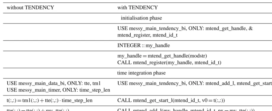
Table 1. Required modification of submodels. The example shows the modification of the total temperature tendency tte. The left column
shows the typical classical code, the right column the TENDENCY approach. The value from the time step before ist m1, the local variablet
is the current (start) value, and my_tte is the new, additional tendency, also a local variable. The time step length is time_step_len and modstr denotes the name of the respective submodel. Note that the “_l” suffix of mtend_add and mtend_get_start are due to different possible entry points with access to different ranks of the variables (here 2-D, see Sect. 2.3).
without TENDENCY with TENDENCY initialisation phase
USE messy_main_tendency_bi, ONLY: mtend_get_handle, & mtend_register, mtend_id_t
INTEGER::my_handle
my_handle=mtend_get_handle(modstr) CALL mtend_register(my_handle, mtend_id_t) time integration phase
USE messy_main_data_bi, ONLY: tte, tm1 USE messy_main_tendency_bi, ONLY: mtend_add_l, mtend_get_start_l USE messy_main_timer, ONLY: time_step_len
t(:,:)=tm1(:,:)+tte(:,:)·time_step_len CALL mtend_get_start_l(mtend_id_t, v0=t(:,:))
tte(:,:)=tte(:,:)+my_tte(:,:) CALL mtend_add_l(my_handle, mtend_id_t, px=my_tte(:,:))
and the possible process–prognostic variable pairs have to be registered already during the initialisation phase of the TEN-DENCY module itself (see also Sect. 2.1).
A second EMAC specific is owed to the spectral trans-form dynamical core of the ECHAM5 base model: the wind speed is usually in units of m s−1, but to meet the needs of the spectral transform on the sphere, it has to be scaled with the cosine of the latitude. Various physical subroutines in the EMAC model, however, perform with the unscaled wind speed. Within TENDENCY, always the scaled wind speed is used. To avoid inconsistencies, TENDENCY provides the subroutine mtend_set_sqcst_scal, which is used to set an internal logical switch telling TENDENCY whether the incoming wind tendency is scaled or not.
The third EMAC specific is related to the dimensions of the prognostic variables in 3-D grid-point space. The ECHAM5 base model uses a specific order of dimensions ((h1, z, h2) whereh1andh2denote the horizontal andzthe vertical dimensions) for code optimisation. Hereby some of the processes perform within a loop over the outer horizontal dimension h2. Therefore, a distinction had to be made be-tween those processes being called globally (outside theh2 loop) and those being called locally (inside theh2loop). In the TENDENCY submodel this issue occurs during the time integration phase, i.e. concerning themtend_get_start
and the mtend_addsubroutines. Here, the arrays have to be of rank 2 ((h1, z)), if called inside the local loop, and of rank 3 ((h1, z, h2)), if called outside. Therefore both subrou-tines are found twice in the TENDENCY module suffixed by either_l(for local) or_g(for global), and differing only by the rank of the array arguments.
3 Diagnostic methods with TENDENCY
The implementation of the MESSy generic submodel TEN-DENCY provides several benefits concerning the handling of the process-based tendency data. The CHANNEL infras-tructure allows a flexible and user-defined output of the infor-mation and thus the memory requirement can be minimised depending on the specific needs. This section describes the independent modes of operation, how the information can be extracted by the user and the optional closure test.
The limitations of the bookkeeping of process tendencies, by design, is the partitioning of the individual processes, ac-cording to the operator splitting concept. If a process can be subdivided into further sub-processes, each calculating a dis-tinct contribution to the tendency, those sub-process tenden-cies can be handled by TENDENCY. This also implies that intermediate tendencies within an implicit scheme cannot be captured by TENDENCY, unless they are explicitly calcu-lated within the scheme.
3.1 User interface
The TENDENCY submodel provides various options for the user to receive data output, which have to be set prior to the model simulation. This is realised via two interfaces con-nected with the module, the corresponding coupling (CPL) namelist and the integrated subroutinemtend_request.
The CPL-namelist contains three logical parameters: – l_full_diagenables the full diagnostic output, i.e.
requires considerably large memory and has been mainly implemented for debugging purposes.
– l_closureenables the internal closure test and cre-ates the additional channel “tendency_clsr” with the two objects required for the closure test (see Sect. 3.2). This test has been implemented to check if all submodels in a given model setup work correctly with respect to the tendency accounting.
– l_clos_diagenables additional output of informa-tion during the model simulainforma-tion into the log file. This contains the external and the internal tendencies (for ex-planation see Sect. 3.2) as well as their difference and is mostly used for development and debugging purposes, e.g. when including a new submodel.
Individual tendency diagnostics can be requested in the CPL-namelist with entries looking like
TDIAG(i)=“X”,“p1;p2+p3;. . .;pn”,
where iis an arbitrary but unique number, X is the name of the prognostic variable (or tracer), andp1topnare the names of the processes (see Sect. 2.1). TENDENCY cre-ates a new output channel (named “tendency_diag”) and one channel object for each semicolon separated list of process sums. These objects either contain the individual tendency of the process–variable pair (examplep1), or the sum of ten-dencies of the corresponding processes (example p2+p3). An additional “unaccounted” object is created, which con-tains the sum of all process tendencies missing in the list. If the “unaccounted” object is zero for all time steps in every grid box, all processes influencing the variableXare within the set of processesp1topn. With this feature, tailor-made diagnostics excerpting only the desired tendencies, thus with a minimised memory requirement, can be set up.
Besides the CPL-namelist controlled generation of new output objects containing individual process tendencies (or sums thereof), TENDENCY also provides an interface sub-routine to enable the access to individual process tendencies by other submodels. Callingmtend_requestfrom the en-try point “init_coupling” of submodel A with the name of the desired submodel B and the identifier of the desired prognos-tic variableXwill generate a new channel object in the chan-nel “tendency_exch” (for exchange) and return a pointer to its memory. If the corresponding process submodel B will commit its tendency by callingmtend_add, this tendency will be copied into this new channel object and therefore be available in submodel A for further calculations.
As for each of the possible modes of operation of the TEN-DENCY submodel an individual channel is generated, they do not exclude or influence each other, but rather work inde-pendently.
3.2 Closure test
An optional closure test can be performed with the TEN-DENCY submodel for every time step during the simu-lation. The test is mainly implemented for development tasks like including new submodels to the TENDENCY structure. If activated via the namelist (see Sect. 3.1), two additional process handles (I_HANDLE_SUM and I_HANDLE_DIFF) are defined. Further, a separate nel “tendency_clsr” is created with corresponding chan-nel objects, two (“sum” and “difference”) for each prog-nostic variable. The “sum” objects are updated every time a tendency is updated in themtend_addsubroutines and thus display the total sum of tendencies, which are cal-culated only within the TENDENCY module (in the fol-lowing called “internal tendency”). As with TENDENCY the total model tendency (in the following called “exter-nal tendency”) should be calculated only within the TEN-DENCY submodel, those two values are supposed to be equal. If these two values differ, the respective variable must be altered by another process of which the tendency com-putation was not relocated to the TENDENCY submodel. Testing this denotes the closure test which is conducted as follows: the channel objects corresponding to the han-dle I_HANDLE_DIFF are used to store the difference be-tween the two tendency values calculated in the subroutine
main_tendency_global_endby subtracting the inter-nal from the exterinter-nal tendency. This difference is used in the subroutinecompute_eps_and_clear. In this sub-routine anεis calculated by
ε=(max|xt ee|)·10−10, (1)
wherext ee denotes the external tendency of the variable or
tracerx. Next, the difference between the two tendencies is challenged to be smaller thanε. If so, certainty is given that all processes changing the respective prognostic variable are properly captured by the TENDENCY submodel. If not, an error message will occur in the log file.
4 Runtime performance analysis
Including the TENDENCY submodel into the EMAC model leads to a number of additional subroutine calls during the simulation. To estimate the extra computing time the EMAC model requires for these, a runtime performance analysis has been conducted. For this, four model simulations (with EMAC version 2.42) over 10 model days with a time step of 15 min were carried out on 1 node with 64 tasks per node on the “blizzard” IBM Power 6 of the DKRZ (Deutsches Kli-marechenzentrum) in Hamburg. While in two of the four sim-ulations the TENDENCY submodel was performing, in the other two it was switched off.
Figure 3. Time series of the average over the 5◦S–5◦N latitudinal band of the specific humidity (in mg kg−1).
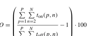
ECHAM5 base model and the basic submodels of the MESSy system (namely: cloud, convect, cvtrans, h2o and rad4all) as well as the extra routines for the middle atmo-sphere (gwspect, ssodrag). In order to receive comparable results, apart from the wall clock no data output was enabled and due to the initialisation phase of the model the first time step was not taken into consideration. For the calculation, the sum of the wall clock time has been taken for every MPI3 parallel task and for every time step of one model simulation. The equation
O=
P P
p=1
N P
n=2
ton(p, n)
P P
p=1
N P
n=2
toff(p, n) −1
·100 (2)
yields the averaged value of the overhead (O) produced by the additional submodel per time step in percent. Here,n in-dicates the time step,P the number of MPI tasks andtonand toffrepresent the wall clock time for the simulations with the TENDENCY submodel either switched on or off. In our tests the use of the TENDENCY submodel results in an additional 1.8±1 % of computing time for the EMAC model in the de-scribed setup.
5 Exemplary results
Exemplarily for presenting a possible application of the TENDENCY submodel the analysis of simulated strato-spheric water vapour (q) has been chosen. Figure 3 shows the simulated representation of the well-known tropical (5◦N– 5◦S) tape recorder signal between 100 and 10 hPa for three simulated years, which was first discovered by Mote et al. (1995, 1996) and Weinstock et al. (1995). For this, we carried out a model simulation in T42L90MA resolution (2.8◦×2.8◦,
3message passing interface
Figure 4. Time series of the average over the 5◦S–5◦N latitudinal band of the total tendency (in ng kg−1s−1) of the specific humidity.
90 vertical layers) initialised from a previous long-term sim-ulation. Only the basic MESSy submodels (convect, cloud, cvtrans, rad4all, tropop) and the ECHAM5 base model are used plus the submodel h2o, which provides a simple pre-scribed water vapour production accounting for the methane oxidation in the stratosphere.
In Fig. 4 the total tendency of the water vapour is shown for the simulated time period. Here a fairly clear distinction can be made between reddish (increasing water vapour) and bluish (decreasing water vapour) patches. These in fact cor-respond to the increasing and decreasing specific humidity over time in Fig. 3. White patches in Fig. 4 correspond to the maxima and minima in Fig. 3. The signal of the total ten-dency also propagates upward in time, like the actual tape recorder signal. At a pressure lower than 30 hPa, the signal dissolves or mixes in with less clear patterns in the upper stratosphere.
Figures 5–9 show the process-based tendencies retrieved via the TENDENCY submodel. For this the line
TDIAG(2)=
“q”,“vdiff;cloud;convect;advect;h2o”, was included into the CPL namelist. As explained in Sect. 3 this generates an output file for the process tendencies of the specific humidityq for each of the five stated submodels, involved in controlling the prognostic development ofq. The sixth generated output object accounting for the unaccounted submodels was tested to be zero at any time and location, to assure that all the processes influencing the specific humidity have been captured.
Figure 5. Time series of the average over the 5◦S–5◦N latitudi-nal band of the large-scale cloud tendency (in ng kg−1s−1) of the specific humidity.
convection submodel (convect) and due to evaporation and sublimation of transported liquid or ice water in the cloud submodel.
Figure 7 shows the impact of the vertical diffusion (vd-iff ). A strong signal goes up to 80 hPa. Above that region, the signal is considerably weaker. The vertical diffusion ten-dencies are about three orders of magnitude smaller than the total tendencies. Above 50 hPa there are almost no changes caused by vertical diffusion, apart from a downward propa-gating signal. It seems to be in phase with the quasi-biannual oscillation (QBO), which may influence the strength of the tape recorder signal (Niwano et al., 2003).
The prescribed water vapour production caused by methane oxidation is shown in Fig. 8. The continuous pro-duction of water vapour from the chemical reactions in-creases with height and varies slightly with season. The mag-nitude of the tendencies are about one order of magmag-nitude smaller than the maxima of the total tendencies.
The advection tendency of the specific humidity can be seen in Fig. 9. It reproduces the tendency tape recorder sig-nal from the total specific humidity tendency in Fig. 4 fairly well, but is weaker. The advection tendency indicates upward propagation from 80 to 30 hPa where it fades out. In the up-per stratosphere the advection tendencies also resemble the total tendencies, but with reduced magnitude.
Figure 10 shows the 3-year temporal and zonal averages of the individual tendencies at the Equator, to provide a pic-ture of the net effect of the processes over the entire sim-ulated period. Here again it can be seen that the influence of the two cloud processes and of the vertical diffusion fade out above the tropopause and the water vapour production by methane oxidation simply increases with height. The av-eraged advection tendency changes from positive to negative values at around 50 hPa and above balances the chemically produced water vapour. As the methane oxidation provides a constant signal it has the same net effect as the advective impact when temporally averaged, even though the maxima are one order of magnitude smaller. Without the chemical
Figure 6. Time series of the average over the 5◦S–5◦N latitudi-nal band of the convective cloud tendency (in ng kg−1s−1) of the specific humidity.
Figure 7. Time series of the average over the 5◦S–5◦N latitudi-nal band of the vertical diffusion tendency (in ng kg−1s−1) of the specific humidity.
Figure 8. Time series of the average over the 5◦S–5◦N latitudi-nal band of the methane oxidation tendency (in ng kg−1s−1) of the specific humidity.
6 Summary
We developed the generic submodel TENDENCY for accessing process-based tendencies of state variables (including tracers) for Earth system models in a well struc-tured manner, with minimum memory requirements and maximum flexibility and user friendliness. Implemented in the EMAC model this Fortran 95 module enables us to diag-nose and to use these process tendencies and thus to simplify the analyses of mechanisms as well as the computation of de-pendent processes. Another advantage of the new submodel is the reduced error susceptibility of the model system, ob-tained by the standardisation of the start value calculation and tendency accounting and by the additional, optional clo-sure test.
The implementation is based on the relocation of the state variable tendency accounting from the submodel of the re-spective process to the tendency module itself. This allows us to directly keep a record of all the process–variable tendency pairs and to output and transfer tailor-made subsets for di-agnostics and further analyses. This generalised approach is less error prone and more user friendly, because no recoding is required to set up specific tendency diagnostics. New sub-models can easily be equipped with the TENDENCY feature by following a simple coding standard. Due to the indepen-dence of the time integration scheme, the concept of TEN-DENCY is also applicable to other base models.
With a computing time overhead of less than 2 % in aver-age for a setup without atmospheric chemistry of the EMAC model due to the additional subroutine calls, we achieved a computationally light implementation of the additional tool. Exemplary results from a 3-year model simulation show the different process tendencies of water vapour in the strato-sphere. Here we see that it is the chemical and the advection tendencies which control the dissipation of the tropical tape recorder signal with height over time.
Figure 9. Time series of the average over the 5◦S–5◦N latitudi-nal band of the advection tendency (in ng kg−1s−1) of the specific humidity.
Figure 10. Zonally averaged process tendencies of the specific
hu-midity (in ng kg−1s−1) at the Equator, averaged over the 3-year time period.
Code availability
TENDENCY is part of the Modular Earth Submodel System (MESSy) since version 2.42. MESSy is continuously further developed and applied by a consortium of institutions. The usage of MESSy and access to the source code is licensed to all affiliates of institutions which are members of the MESSy Consortium. Institutions can be a member of the MESSy Consortium by signing the MESSy Memorandum of Un-derstanding. More information can be found on the MESSy Consortium Website (http://www.messy-interface.org).
The Supplement related to this article is available online at doi:10.5194/gmd-7-1573-2014-supplement.
Acknowledgements. The authors thank the DFG (Deutsche
Research Unit 1095); the presented development was conducted as part of R. Eichinger’s PhD thesis under grant number BR 1559/5-1. We acknowledge support from the German Climate Computing Centre (DKRZ) and thank all MESSy developers and submodel maintainers for their support. Furthermore, we thank M. Ponater and S. Brinkop for valuable comments on the manuscript draft and K. Ketelsen for initiating the basic idea. We also thank A. Grini and an anonymous referee for their constructive reviews of the manuscript.
The service charges for this open access publication have been covered by a Research Centre of the Helmholtz Association.
Edited by: O. Boucher
References
Jöckel, P., Sander, R., Kerkweg, A., Tost, H., and Lelieveld, J.: Tech-nical Note: The Modular Earth Submodel System (MESSy) – a new approach towards Earth System Modeling, Atmos. Chem. Phys., 5, 433–444, doi:10.5194/acp-5-433-2005, 2005.
Jöckel, P., Kerkweg, A., Buchholz-Dietsch, J., Tost, H., Sander, R., and Pozzer, A.: Technical Note: Coupling of chemical processes with the Modular Earth Submodel System (MESSy) submodel TRACER, Atmos. Chem. Phys., 8, 1677–1687, doi:10.5194/acp-8-1677-2008, 2008.
Jöckel, P., Kerkweg, A., Pozzer, A., Sander, R., Tost, H., Riede, H., Baumgaertner, A., Gromov, S., and Kern, B.: Development cycle 2 of the Modular Earth Submodel System (MESSy2), Geosci. Model Dev., 3, 717–752, doi:10.5194/gmd-3-717-2010, 2010. Mote, P., Rosenlof, K., Holton, J., Harwood, R., and Waters, J.:
Sea-sonal variations of water vapor in the tropical lower stratosphere, Geophys. Res. Lett., 9, 1093–1096, 1995.
Mote, P., Rosenlof, K., Mclntyre, M., Carr, E., Gille, J., Holton, J., Kinnersley, J., Pumphrey, H., Russel, J., and Waters, J.: An at-mospheric tape recorder: the imprint of tropical tropopause tem-peratures on stratospheric water vapor, J. Geophys. Res., 101, 3989–4006, 1996.
Niwano, M., Yamazaki, K., and Shiotani, M.: Seasonal and QBO variations of ascent rate in the tropical lower stratosphere as in-ferred from UARS HALOE trace gas data, J. Geophys. Res., 108, 4794, doi:10.1029/2003JD003871, 2003.