doi:10.5194/gmd-10-1521-2017
© Author(s) 2017. CC Attribution 3.0 License.
Collection/aggregation algorithms in Lagrangian cloud
microphysical models: rigorous evaluation in box model simulations
Simon Unterstrasser1, Fabian Hoffmann2, and Marion Lerch11Deutsches Zentrum für Luft- und Raumfahrt (DLR) – Institut für Physik der Atmosphäre, Oberpfaffenhofen,
82234 Wessling, Germany
2Leibniz Universität Hannover – Institute of Meteorology and Climatology, 30419 Hannover, Germany
Correspondence to:Simon Unterstrasser ([email protected]) Received: 17 October 2016 – Discussion started: 28 November 2016
Revised: 3 March 2017 – Accepted: 16 March 2017 – Published: 13 April 2017
Abstract.Recently, several Lagrangian microphysical mod-els have been developed which use a large number of (com-putational) particles to represent a cloud. In particular, the collision process leading to coalescence of cloud droplets or aggregation of ice crystals is implemented differently in var-ious models. Three existing implementations are reviewed and extended, and their performance is evaluated by a com-parison with well-established analytical and bin model solu-tions. In this first step of rigorous evaluation, box model sim-ulations, with collection/aggregation being the only process considered, have been performed for the three well-known kernels of Golovin, Long and Hall.
Besides numerical parameters, like the time step and the number of simulation particles (SIPs) used, the details of how the initial SIP ensemble is created from a prescribed analyt-ically defined size distribution is crucial for the performance of the algorithms. Using a constant weight technique, as done in previous studies, greatly underestimates the quality of the algorithms. Using better initialisation techniques consider-ably reduces the number of required SIPs to obtain realistic results. From the box model results, recommendations for the collection/aggregation implementation in higher dimensional model setups are derived. Suitable algorithms are equally rel-evant to treating the warm rain process and aggregation in cirrus.
1 Introduction
The collection of cloud droplets and the aggregation of ice crystals are important processes in liquid and ice clouds. By changing the size, number and, in the case of ice, the shape of hydrometeors, collection and aggregation affect the mi-crophysical behaviour of clouds and thereby their role in the climate system.
The warm rain process (i.e. the production of precipita-tion in clouds in the absence of ice) depends essentially on the collision and subsequent coalescence of cloud droplets. At its initial stage, however, condensational growth governs the activation of aerosols and the following growth of cloud droplets, which might initiate the collection process if they become sufficiently large. Then, collection produces drizzle or raindrops, which are able to precipitate from the cloud, affecting lifetime and organisation of clouds (e.g. Albrecht, 1989; Xue et al., 2008).
In ice clouds, sedimentation, deposition growth and in par-ticular radiative properties depend on the ice crystals’ habits (Sölch and Kärcher, 2011, and references therein). Ice aggre-gates scatter shortwave radiation more strongly than pure ice crystals of the same mass. Recent simulation results suggest that contrail cirrus and natural cirrus can be strongly interwo-ven. In the mixing area, with ice crystals of both origins being present, a prominent bimodal spectrum occurs and enhances the probability of collisions (Unterstrasser et al., 2016).
equation, Smoluchowski or population balance equation (e.g. Wang et al., 2007). It yields
∂fm(m, t )
∂t =
1 2
m Z
0
K(m0, m−m0)fm(m0, t )fm(m−m0, t )dm0
− ∞ Z
0
K(m, m0)fm(m, t )fm(m0, t )dm0, (1)
wherefm(m)dmis the number concentration within an
in-finitesimal interval around the mass m. The first term (gain
term) accounts for the coalescence of two smaller droplets forming a new droplet with mass m; the second term (loss
term) accounts for the coalescence of droplets with massm
with any other droplets forming a larger droplet. The col-lection kernel K(m, m0) describes the rate by which
col-lections between a droplet with mass mand a droplet with
massm0occur. Due to the symmetry of the collection kernel
(K(m, m0)=K(m0, m)) the first term on the right-hand side
can also be written asRm/2
0 K(m0, m−m0)fm(m0, t )fm(m− m0, t )dm0.
For several kernel functions (mostly of polynomial form), analytic solutions exist for specific initial distributions (Golovin, 1963; Berry, 1967; Scott, 1968). The Golovin ker-nel (sum of masses) is given by
K(m, m0)=b (m+m0). (2)
Solutions for more realistic kernels (Long, 1974; Hall, 1980; Wang et al., 2006) and arbitrary initial distribution can be obtained with various numerical methods mainly using a bin representation of the droplet size distribution (Berry and Reinhardt, 1974; Tzivion et al., 1987; Bott, 1998; Simmel et al., 2002; Wang et al., 2007). The hydrodynamic kernel is defined as
K(r, r0)=π(r+r0)2 |wsed(r)−wsed(r0)| Ec(r, r0), (3)
based on the radius r and the sedimentation velocitywsed.
Parametrisations of the collection efficiency Ec are given,
e.g. by Long (1974) or Hall (1980). In the above formula, the differential sedimentation is the driver of collections. No same-size collisions can occur, i.e.K(r, r)=0. More
sophis-ticated expressions forK(r, r0)have been derived to include
turbulence enhancement of the collisional growth, which also allow same-size collisions (K(r, r) >0) (e.g. Ayala et al.,
2008; Grabowski and Wang, 2013; Chen et al., 2016). Solving (1) demands simplifications in the representation of the droplet spectrum for which several numerical models have been developed. Spectral-bin models (e.g. Khain et al., 2000) represent the spectrum by dividing it into several in-tervals (so-called bins). This approach enables the prediction of the temporal development of the droplet number concen-tration in each bin by using the method of finite differences (e.g. Bott, 1998). The accuracy of these models is primarily
determined by the number of used bins (usually on the order of 100), which makes them computationally challenging and prohibits their use in day-to-day applications like numerical weather prediction. Less challenging but less accurate are cloud microphysical bulk models that compute the tempo-ral change of integtempo-ral quantities of the droplet spectrum (e.g. Kessler, 1969; Khairoutdinov and Kogan, 2000; Seifert and Beheng, 2001). These are usually equations for the temporal evolution of bulk mass (so-called one-moment schemes) and additionally number concentration (two-moment schemes) or radar reflectivity (three-moment schemes), which describe the change of the entities of cloud droplets and rain drops (in the case of warm clouds). The separation radius between cloud droplets and rain drops depends on the details of the bulk scheme, but generally cloud droplets (up to 20 to 40 µm in radius) are assumed to have negligible sedimentation fall velocities, while larger drops, frequently subsumed as rain drops, have a sufficient sedimentation velocity to cause colli-sion/coalescence. The interactions of cloud and rain drops are therefore described in terms of self-collection (coales-cence of cloud (rain) drops resulting in cloud (rain) drops), autoconversion (coalescence of cloud droplets resulting in rain drops) and accretion (collection of cloud droplets by rain drops). A third alternative for computing cloud micro-physics has been developed in the recent years: Lagrangian cloud models (LCMs). These models represent cloud micro-physics on the basis of individual computational particles (SIPs). Similar to spectral-bin models, LCMs enable the de-tailed representation of droplet spectra.
their relative novelty due to their higher computational de-mand. Many aspects of this approach have not been validated adequately and there is potential for future improvements. For the process of collection/aggregation, this study will of-fer a first rigorous evaluation of the available numerical ap-proaches.
To our knowledge, five fully coupled LCMs for warm clouds exist, which are described in Andrejczuk et al. (2008), Shima et al. (2009), Riechelmann et al. (2012), Arabas et al. (2015) and Naumann and Seifert (2015), and have been extended or applied in various problems (e.g. Andrejczuk et al., 2010; Arabas and Shima, 2013; Lee et al., 2014; Hoffmann et al., 2015). For ice clouds, three models exist (Paoli et al., 2004; Shirgaonkar and Lele, 2006; Sölch and Kärcher, 2010) which have been applied to natural cirrus (Sölch and Kärcher, 2011) and, in particular, to contrails (e.g. Paoli et al., 2013; Unterstrasser, 2014; Unterstrasser and Görsch, 2014). In the context of ice clouds and warm clouds, different names are used for processes that are simi-lar, in particular in terms of their numerical treatment (depo-sition/sublimation vs. condensation/evaporation, collection vs. aggregation). Conceptually similar are particle-based ap-proaches in aerosol physics (Riemer et al., 2009; Maisels et al., 2004) which account for coagulation of aerosols (DeV-ille et al., 2011; Kolodko and Sabelfeld, 2003).
So far, no consistent terminology has been used in the lat-ter publications. Various names have been used for the same things by various authors. We point out that super droplet, computational droplet and simulation particle (SIP) all have the same meaning and refer to several identical real cloud droplets (or ice crystals) represented by one Lagrangian par-ticle. The number of real droplets represented in a SIP is denoted as the weighting factor or multiplicity. Moreover, Lagrangian approaches in cloud physics have been named the Lagrangian cloud model (LCM), super droplet method (SDM) or particle-based method. In this paper, we use the terms SIP, weighting factor νsim and LCM. Here, droplet
refers to either real droplets or ice crystals. If we say in the following that “SIPiis larger than SIPj”, this means that the
droplets represented in SIPiare larger than those in SIPj.
Such a statement it is not related to the weighting factor of the SIPs.
Usually, only the liquid water or the ice of a cloud are de-scribed with a Lagrangian representation, whereas all other physical quantities (like velocity, temperature and water vapour concentration) are described in Eulerian space (see also discussion in Hoffmann, 2016). SIPs have discrete po-sitions xp=(xp, yp, zp)within a grid box. The position is
regularly updated, obeying the transport equation∂xp/∂t= u. Microphysical processes like sedimentation and droplet
growth are treated individually for each SIP. Interpolation methods can be used to evaluate the Eulerian fields at the specific SIP positions. This implicitly assumes that all νsim
droplets of the SIPs are located at the same position. On the other hand, the droplets of a SIP are assumed to be
well-mixed in the grid box in the LCM treatment of collection and sometimes condensation. Then, the number concentra-tion represented by a single SIP, e.g. is given byνsim/1V,
where1V is the volume of the grid box.
Lists of used symbols and abbreviation are given in Ta-bles 1 and 2.
2 Description of the various collection/aggregation implementations
We use the terminology of Berry (1967), where fln r and gln r denote the number and mass density function with
re-spect to the logarithm of droplet radius lnr. The relations gln r(r)=mfln r(r) andflnr(r)=3mfm(m) hold. The lat-ter designates the number density function with respect to mass and obeys the transformation property of distributions:
fy(y)dy=fx(x(y))dx. For consistency with previous
stud-ies,gln ris used for plotting purposes, whereasfm andgm
are more relevant in the following analytical derivations. The moments of order k of the mass distribution fm
(equivalent to the number density function with respect to mass) are defined as
λk(t )= Z
mkfm(m, t )dm. (4)
The low-order moments represent the droplet number con-centration (DNC=λ0) and the mass concentration (liquid
water content; LWC=λ1). The analogous extensive
proper-tiesλk(t ) 1V are the total droplet numberN, total droplet massMand radar reflectivity (Z=λ2 1V). For a given SIP
ensemble, the moments can be computed by
λk,SIP(t )= NSIP X
i=1
νiµik ! ,
1V , (5)
whereµi is the single droplet mass of SIPiandNSIP is the number of SIPs inside a grid box. For reasons of consistency with Wang et al. (2007), we translate the SIP ensemble into a mass distributiongmin bin representation and then compute
the moments with the formula
λk,BIN(t )= NBIN X
i=1
gm(mi, t )(mebb,l) k−1ln10
3κ (6)
(cf. with their Eq. 48).
The initialisation is successful for a given parameter set if the moments of the SIP ensembleλk,SIP are close to the analytical valuesλk,anal. For an exponential distribution (as used in this study), the probability density function (PDF) reads as
fm(m)= N
1Vm¯ exp
−m
¯ m
; (7)
the moments are given analytically by
Table 1.List of symbols.
Symbol Value/unit Meaning
fm,fem kg−1m−3, 1 (normalised) droplet number concentration per mass interval
gm, gln r m−3, kg m−3 droplet mass concentration per mass interval/per logarithmic radius interval
m, m0 kg mass of a single real droplet
mbb kg bin boundaries of the bin grid
¯
m=λ1/λ0=M/N kg mean mass of all droplets
nbin,l 1 droplet number in binl
r, r0 m droplet radius
rlb m threshold radius inνrandom,lb-init
rcritmin m lower cut-off radius in singleSIP-init
wsed m s−1 sedimentation velocity
DNC=λ0 m−3 droplet number concentration
Ec 1 collection/aggregation efficiency
K m3s−1 collection/aggregation kernel
LWC=λ1 kg m−3 droplet mass concentration, liquid water content
Mbin,l kg total droplet mass in binl
NSIP 1 number of SIPs
NBIN 1 number of bins
αlow, αmed, αhigh 1 parameters of theνrandom-init method
1t s time step
1V m3 grid box volume
η 1 parameter in RMA and singleSIP-init method
κ 1 number of bins per mass decade
λk kgkm−3 moments of the orderk
µ kg single droplet mass of a SIP
νcritmax 1 maximum number of droplets represented by a SIP
νcritmin 1 minimum number of droplets represented by a SIP
ν 1 number of droplets represented by a SIP
ξ 1 splitting parameter of AON
χ=µ ν, eχ=χ /M kg, 1 total droplet mass of a SIP
N =λ01V 1 total droplet number
M=λ11V kg total droplet mass
Z=λ21V kg2 second moment of droplet mass distribution (radar reflectivity)
Table 2.List of abbreviations.
AON All-or-nothing algorithm AIM Average impact algorithm DSD Droplet size distribution LCM Lagrangian cloud model PDF Probability density function RMA Remapping algorithm
OTF Update on the fly RedLim Reduction limiter
SIP Simulation particle
wherek!is the factorial ofkandm¯ =M/N the mean mass
(Rade and Westergren, 2000).
Throughout this study, the initial parameters of the droplet size distribution (DSD) are DNC0=2.97×10⁸m−3 and
LWC0=10−3kg m−3 (implying a mean radius of 9.3 µm)
as in Wang et al. (2007). The higher moments are λ2,anal=
6.74×10⁻¹⁵kg2m−3andλ3,anal=6.81×10⁻²⁶kg3m−3.
2.1 Initialisation
2.1.1 SingleSIP-init and multiSIP-init
First, the mass distribution is discretized on a logarith-mic scale. The boundaries of bin l are given by mbb,l=
mlow10l/κandmbb,l+1, wheremlowis the minimum droplet mass considered. The bin centre is computed using the arith-metic mean m¯bb,l=0.5(mbb,l+1+mbb,l). The bin size is
1mbb,l=(mbb,l+1−mbb,l). The mass increases 10-fold ev-eryκbin. Several previous studies used the parameterswith mbb,l+1/mbb,l=21/s to characterise the bin resolution. The parameterssandκare related vias=κ log10(2)≈0.3 κ.
For each bin, the droplet number is approximated by
νb=fm(m¯bb,l) 1mbb,l1V, and one SIP with weighting fac-tor νsim=νb and droplet mass µsim= ¯mbb,l is created if
νb is greater than a lower cut-off threshold νcritmin. No
SIP is created if νb< νcritmin. Moreover, no SIPs are
cre-ated from bins with radiusr < rcritmin. We will refer to this
as deterministic singleSIP-init. In its probabilistic version, the mass µsim is randomly chosen within each bin l and νsim=fm(µsim) 1mbb,l1V is adapted accordingly. By de-fault, rcritmin=0.6 µm andνcritmin=η×νmax, which is
de-termined from the maximal weighting factor within the entire SIP ensembleνmaxand the prescribed ratio of the minimal to
the maximal weighting factor η=10−9. For largerrcritmin,
it is advantageous to initialise one additional “residual” SIP that contains the sum of all neglected contributions.
Following Unterstrasser and Sölch (2014, see their Ap-pendix A), we introduce the multiSIP-init technique. It is similar to the singleSIP-init technique, except that we addi-tionally introduce an upper thresholdνcritmax. Ifνb> νcritmax
is fulfilled for a specific bin, then this bin is divided into
κsub= dνb/νcritmaxe sub-bins and a SIP is created for each
sub-bin. The multiSIP-init technique gives a good trade-off between resolving low concentrations at the DSD tails and high concentrations of the most abundant droplet masses. By default,νcritmax=0.1νmax.
So far, we introduced initialisation techniques with a strict lower threshold νcritmin with no SIPs created in bins with νb< νcritmin. We can relax this condition by introducing –
what we call – a weak threshold. This means that, in such a low-contribution bin (with νb< νcritmin), we create a SIP
with the probability pcreate=νb/νcritminand weighting
fac-torνsim=νcritmin. Having many realisations of initial SIP
en-sembles, the expectation value of the droplet number repre-sented by such SIPs,νcritmin·pcreate+0·(1−pcreate), equals the
analytically prescribed valueνb. Using a strict threshold the
droplet number would be simply 0 in those low-contribution bins. In a related problem, such a probabilistic approach has been shown to strongly leverage the sensitivity of ice crystal nucleation on the numerical parameterνcritmin. This led to a
substantial reduction of the number of SIPs that are required for converging simulation results (Unterstrasser and Sölch, 2014).
Using the probabilistic version and a weak lower thresh-old is particularly important if different realisations of SIP
ensembles of the same analytic DSD should be created. The number of SIPsNSIPdepends onκ,νcritmin,νcritmaxand the
parameters of the prescribed distribution.
Moreover, the singleSIP-init is used in a hybrid version, where differentκvalues are used in specified radius ranges.
Table 3 lists the resulting number of SIPs for the range of
κvalues used in simulations with the probabilistic
singleSIP-init and variants of it.
2.1.2 νconst-init andνdraw-init
The accumulated PDFF (m)is given byR0mfem(m0)dm0with the normalised PDFfem=fm/λ0. First, the sizeNSIPof the SIP ensemble that should approximate the initial DSD is specified. For each SIP, its massµiis reasonably picked by
µi=F−1(rand()), (9)
where rand() generates uniformly distributed random num-bers ∈ [0,1]. In the case of the νconst-init, the weighting
factors of all SIPs are equallyνi =νconst=N/NSIP. This init method reproduces SIP ensembles similar to the ones in Shima et al. (2009) or Hoffmann et al. (2015). As a variety of theνconst-init method, the weighting factorsνi in theνdraw -init method are simply perturbed byνi=2 rand() νconst.
For the case of an exponential distribution, the following holds for the SIPsi=1, NSIP:
µi= − ¯mlog(rand()). (10)
In the literature, this approach is known as inverse transform sampling. A proof of correctness can be found in classical textbooks, e.g. Devroye (1986, their Sect. II.2).
2.1.3 νrandom-init
The third approach allows specifying the spectrum of weight-ing factors that should be covered by the SIP ensem-ble. Similar to the νdraw-init method, the weighting
fac-tors are randomly determined. Whereas the latter method produced a SIP ensemble with weighting factors uniformly distributed in ν, the νrandom-init produces weighting
fac-tors uniformly distributed in log(ν)and covering the range [N 10αlow, N 10αhigh]. The eventual number of SIPs de-pends most sensitively on the parameterαhigh, which controls
how big the portion of a single SIP can be.
SIPs with weighting factors νi=
N 10(αlow+(αhigh−αlow)·rand()) are created until PNSIP j=1νj exceeds N. The weighting factor of the last SIP is cor-rected such that PNSIP
j=1νj=N holds. Now, the mass µi of each SIP is determined by the following technique: the first SIP represents the smallest droplets and covers the mass interval [0, m1], whereas the last SIP
Table 3.Number of SIPs for the probabilistic singleSIP-init method (and variants like the multiSIP-init) as a function ofκ. The given values are averages over 50 realisations and rounded to the nearest integer. The right-most column lists the figures in which simulation results with this specific init method are depicted. SUPP refers to the Supplement of this paper.
κ
5 10 20 40 60 100 200 400
Init method NSIP Figure
SingleSIP 24 49 98 197 296 494 988 1976 10, 12, 14, 18
MultiSIP 256 517 775 1295 19
SingleSIP;rcritmin=1.6 µm 74 149 223 372 19
SingleSIP;rcritmin=3.0 µm 58 116 173 228 SUPP
SingleSIP;rcritmin=5.0 µm 45 89 113 221 SUPP
SingleSIP;tinit=10 min 58 114 227 339 565 SUPP
SingleSIP;tinit=20 min 72 142 284 426 709 21
SingleSIP;tinit=30 min 89 176 352 527 878 SUPP
Rmi
0 fm(m0)dm0 1V =Pij=1νj. The total mass contained in each SIP is given by χi=
Rmi
mi−1fm(m0)m0dm0 1V and the single droplet mass byµi=χi/νi.
For the case of an exponential distribution, the following holds for the interval boundaries and the SIPsi=1, NSIP:
mi= − ¯mlog
N−Pi
j=1νj
N !
(11)
and
µi=
m
i−1− ¯m
exp(mi−1/m)¯ −
mi− ¯m exp(mi/m)¯
N
νi
. (12)
The above formulas, which involve several differences of similarly valued terms, must be carefully implemented such that numerical cancellation errors are kept tolerable.
Experimenting with the SIP-init procedure, several op-timisations have been incorporated. First, the ν
spec-trum is split into two intervals [N 10αlow, N 10αmed] and
[N 10αmed, N 10αhigh]. We alternately pick random values from the two intervals. Without this correction, it happens that several consecutive SIPs with small weights, and hence nearly identical droplet masses, are created, which increases the SIP number without any benefits.
Going through the list of SIPs, the droplet masses increase, and hence the individual SIPs contain gradually increasing fractions of the total grid box mass. This can lead to a rather coarse representation of the right tail of the DSD. Two op-tions to improve this have been implemented. In theνrandom,rs option, the νi values are reduced by some factor that in-creases as Pi
j=1νj approachesN. In theνrandom,lb option,
νvalues are randomly picked up to a certain radius threshold rlb. Above this threshold, SIPs are created with the singleSIP
method with linearly spaced bins.
2.1.4 Comparison
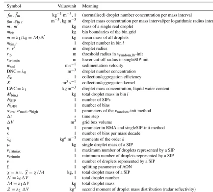
Figure 1 shows the weighting factors and other properties of the initial SIP ensemble, which may affect the perfor-mance of the algorithms. Each column shows one class of initialisation techniques. For a certain realisation, the first row shows the weighting factors νi of all SIPs as a func-tion of their represented droplet radiusri. Each dot shows the (νi, ri) pair of one SIP. For the singleSIP-init, the dots are homogeneously distributed along the horizontal axis, as one SIP is created from each bin (with exponentially increas-ing bin sizes). The accordincreas-ingν values relate directly to the
prescribed DSD. The higherfm1m, the more droplets are
represented in a SIP. No SIPs smaller thanrcritmin=0.6 µm
are initialised and theνvalues range over 9 orders of
magni-tude, consistent withη=10−9. The multiSIP-init introduces
an upper bound ofνcritmax=2.6×10⁶forν. This threshold
is effective over a certain radius range where the SIPs, com-pared to the singleSIP-init, have lowerνvalues and are also
more densely distributed along the horizontal axis. For the
νconst-init, all SIPs useν=νconst, whereas for theνdraw-init
theν values scatter around this value. Forνconst andνdraw,
theνvalues are chosen independently of the given DSD
con-trary to the latter techniques. However, for both techniques, the density of the dots along theraxis is correlated tofm1m.
Theνrandom-init technique randomly picksνvalues which
are distributed over a larger range compared to theνdraw-init.
In fact, they are uniformly distributed in log(ν). The range
of possibleν values can be adjusted and is chosen similar
to the singleSIP/multiSIP by settingαhigh= −2, αmed= −3
andαlow= −7, which are the defaults in all simulations
pre-sented here. The present method is more flexible compared to the singleSIP approach, as the occurrence of certainνvalues
is not limited to a certain radius range. In the singleSIP-init, the smallestνvalues occur only on the left and right tails of
the DSD, whereas in theνrandomapproach the smallestν
Figure 1.Characteristics of the various SIP initialisation methods (as given on top of each panel): weighting factorsνi(ri)of an initial
SIP ensemble, the mean weighting factorsν(r), the occurrence frequency of the¯ νi values and the resulting mass density distributionsglnr are displayed (rows 1 to 4). Row 1 displays data of a single realisation, whereas rows 2 to 4 show averages over 50 SIP ensembles. The bottom row shows the momentsλ0,λ1,λ2andλ3normalised by the respective analytical value. Every symbol depicts the value of a single realisation. The nearly horizontal line connects the mean values over all realisations. In the displayed examples,κ=10 in the singleSIP-init, κ=10, νcritmax≈2.6×10⁶in the multiSIP-init,NSIP=80 in theνconst,νdraw-init and(αhigh, αmed, αlow)=(−2,−3,−7)in theνrandom -inits. In top right panel, the dashed horizontal lines indicate the values ofN 10αlow,N 10αmed andN 10αhighand the dashed vertical line the threshold radiusrlb.
range. The horizontal lines in the top right panel indicate the values ofN 10αlow,N 10αmed andN 10αhigh and the vertical line the threshold radiusrlb.
The second row shows average ν value of all SIPs in a
certain size bin. All init techniques are probabilistic and the average is taken over 50 independent realisations of SIP en-sembles. Not surprisingly, the averageνof theνdrawmethod
is identical to νconst. Moreover, also for theνrandom-init, the
averageνvalue is constant over a large radius range. Only in
the right tail do theνvalues drop as intended. The third row
shows the occurrence frequency of weighting factors. To display DSDs represented by a SIP ensemble, a SIP ensemble must be converted back into a bin representation. For this, we establish a grid with resolution κplot=4 and
count each SIP in its respective bin; i.e. SIPi withmbb,l<
cho-sen in the initialisation. The fourth row shows such DSDs again as an average over 50 SIP ensemble realisations. We find that any init technique is, in general, successful in pro-ducing a meaningful SIP ensemble as the “back”-translated DSD matches the originally prescribed DSD (black). Hence, the moments λk,SIP match the analytical values λk,anal for 0≤k≤3, as shown in the fifth row. Nevertheless, for the νconst- andνdraw-init, the spread between individual
realisa-tions can be large and they deviate substantially from the an-alytical reference. The singleSIP/multiSIP-init andνrandom
-init, on the other hand, guarantee that each individual reali-sation is fairly close to the reference. In the results section, the presented simulations mostly use the probabilistic single-SIP initialisation. Table 3 lists the number of single-SIPs for several init methods and parameter configurations. The right-most column indicates in which figure the simulations using the specific init method are displayed.
2.2 Description of hypothetical algorithm
First, we present a hypothetical algorithm for the treatment of collection/aggregation in an LCM, which would probably yield excellent results. However, it is prohibitively expensive in terms of computing power and memory, asNSIPincreases
drastically over time until the state is reached where each SIP represents exactly one real droplet. Nevertheless, the presen-tation of this algorithm is useful for introducing several con-cepts which will partly occur in the subsequently described “real-world” algorithms.
Whereas condensation/deposition and sedimentation may be computed using interpolated quantities which implicitly assume that all droplets of a SIP are located at the same point, the numerical treatment of collection usually assumes that the droplets of a SIP are spatially uniformly distributed, i.e. well-mixed within the grid box. An approach, where the ver-tical SIP position is retained in the collection algorithm and the process of larger droplets overtaking smaller droplets is explicitly modelled, is described in Sölch and Kärcher (2010) and not treated here.
Following Gillespie (1972) and Shima et al. (2009), the probabilityPij that one droplet with massmi collides with one droplet with massmjinside a small volumeδV within a short time intervalδt is given by
Pij=Kij δt δV−1, (13)
whereKij =K(mi, mj).
For SIPs i andj containing νi andνj real droplets in a grid box with volume1V, on average,νcoll=Pij νi νj col-lections between droplets from SIP iand SIPj occur. The
average rate of suchi−j collections (i6=j) to occur is
∂νcoll(i, j )
∂t =νi Kij νj1V −1=:ν
ioij=:Oij. (14)
So-called self-collections, collisions of the droplets belong-ing to the same SIP (i=j), are described by
∂νcoll(i, i)
∂t =2·
νi 2 Kii
νi 21V−1
=12νi Kii νi1V−1
=:νioii=:Oii, (15)
assuming that the SIP is split into two portions, each contain-ing one-half of the droplets of the original SIP. The factor of 2 originates from the collections of each half, which have to be added to gain the total number of self-collections for SIP
i. Accordingly, the diagonal elements of the matricesoij and
Oij differ from the off-diagonal elements by an additional factor of 0.5. In terms of concentrations (represented by SIPs in a grid box with volume1V), we can write
∂ncoll(i, j )
∂t =Kij ni nj (16)
for collections between different SIPs and
∂ncoll(i, i)
∂t =
1
2 Kii ni2 (17)
for self-collections.
In the hypothetical algorithm, the weighting factor of SIPi
is reduced due to collections with all other SIPs and self-collections and reads as
∂νi
∂t = −
NSIP X
j=1
∂νcoll(i, j )
∂t = −
NSIP X
j=1
Oij. (18)
The droplet massµiin SIPiis unchanged.
For eachi−j combination, a new SIPkis generated: ∂νk
∂t =Oij and µk=µi+µj. (19)
To avoid double counting, only combinations withi ≥j are
considered.
The rate equations for the weighting factors can be numer-ically solved by a simple Euler forward step. The weighting factor of existing SIPs is reduced by
νi1:=
NSIP X
j=1 Oij
!
1t, (20)
leading to
νi∗=νi−νi1, (21)
or, equivalently,
νi∗=νi 1−1t NSIP X
j=1 oij
!
. (22)
For new SIPsk, we have
Per construction, the algorithm is mass conserving subject to rounding errors.
In each time step,NSIP,add=NSIP (NSIP−1)/2, new SIPs are produced and the new number of SIPs isNSIP∗=NSIP+ NSIP,add. Afternttime steps, the number of SIPs would be of order(NSIP,0)nt which is not feasible.
In the following subsections, algorithms are presented that include various approaches to keep the number of SIPs in an acceptable range.
In the following, the various algorithms are described and pseudo-code of the implementations is given. For the sake of readability, the pseudo-code examples show easy-to-understand implementations. The actual codes of the al-gorithms are, however, optimised in terms of computational efficiency. The style conventions for the pseudo-code exam-ples are as follows: commands of the algorithms are written in upright font with keywords in boldface. Comments appear in italic font (explanations are enclosed by {} and headings of code blocks are in boldface).
2.3 Description of the remapping algorithm (RMA) First, the remapping algorithm is described, as its concept follows closely the hypothetical algorithm introduced in the latter section. RMA is based on ideas of Andrejczuk et al. (2010). We call their approach the “remapping algorithm” as NSIP is kept reasonably low by switching between a SIP
representation and a bin representation in every time step. A temporary bin grid with a predefinedκ is established which
stores the total number nbin,∗ and total mass Mbin,∗ of all contributions belonging to a specific bin. The bin boundaries are given bymbb,∗.
Instead of creating a new SIPk(with numberνkobtained by Eq. (19) and massµk=µi+µj) from eachi−j com-bination, the according contribution is stored on a temporary bin grid. More explicitly, this means that the droplet num-bernbin,l of binl withmbb,l< µk≤mbb,l+1is increased by
νk. Similarly, the total massMbin,lof that bin is increased by
µkνk. Similarly, the reduced contributionsν∗i from the exist-ing SIPs with droplet massµi are added to their respective bins.
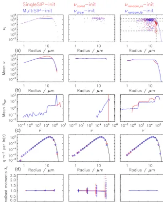
Figure 2 illustrates how a collection process between two SIPs is treated in RMA. In this example, νk=2 droplets are produced by collections which have a droplet mass of
µk=µi+µj=15. Instead of creating a new SIPk (as in the hypothetical algorithm), the contribution k is recorded
in the bin grid. The droplet numbernin binl3 is increased
by νk=2 and the according total mass Ml3 byνkµk=30. The remaining contribution of SIPifalls into binl1 andnl1 andMl1are increased by νi∗=νi−νk=2 and µiνi∗=12, respectively. The operation for SIPj is analogous.
At the end of each time step, after treating all possible
i−j combinations, a SIP ensemble is created from the bin
data withνi=nbin,landµi=Mbin,l/nbin,l, which resembles a deterministic singleSIP-init with the resolutionκ.
Optionally, a lower thresholdνmin,RMAcan be introduced, such that SIP i is created only if nbin,l> νmin,RMA holds. However, this may destroy the property of mass conservation which can be remedied by the following.
We pick up the concept of a weak threshold introduced earlier and adjust it such that on average the total mass is conserved (instead of total number as before). We introduce the thresholdMcritmin=ηλ1. The parameterηis set to 10−8,
which implies that each SIP contains at least a fraction of 10−8 of the total mass in a grid box. If M
bin,l> Mcritmin, a SIP is created representing νi=nbin,l drops with single mass µi=Mbin,l/nbin,l. If Mbin,l< Mcritmin, a SIP is
cre-ated with probabilitypcreate=Mbin,l/Mcritmin. In this case,
the SIP representsνi=Mcritmin/µidroplets with single mass
µi=Mbin,l/nbin,l. Pseudo-code of the algorithm is given in Algorithm (1).
Time steps typically used in previous collec-tion/aggregation tests are around1t=0.1 to 10 s depending
inter alia on the used kernel. From Eq. (22) it follows that the time step in RMA must satisfy
1t <
NSIP X
j=1
oij. (24)
Otherwise, negative ν values can occur which would
in-evitably lead to a crash of the simulation. In mature clouds, the Long and Hall kernels attain large values which required tiny time steps of 10−4s and were smaller in the first test
simulations. To be of any practical relevance, RMA had to be modified in order to be able to run simulations with suit-able time steps.
Hence, several extensions to RMA allowing larger time steps are proposed in the following.
1. The default version uses the algorithm as outlined in Al-gorithm (1) (i.e. nothing is changed). Negativeνi∗values
obtained by Eq. (21) are acceptable, as long asnbin,l,
from which the SIPs are created at the end of the time iteration, is non-negative for alll. This means that an
existing SIP i (which falls into bin l) can lose more
droplets (ν1i ) than it actually possesses (νi) as long as the gain in binl (from all suitable SIP combinations)
compensates this deficit. We will later see that this ap-proach works well for the Golovin kernel; however, it fails for the Long and Hall kernels.
2. Clipping simply ignores bins with negative nbin,l and does not create SIPs from those bins. This approach de-stroys the property of mass conservation and is not pur-sued here.
3. In adaptive time stepping, instead of reducing the gen-eral time step, only the treatment of SIPs withνi∗<0
Algorithm 1Pseudo-code of the Remapping algorithm (RMA); style conventions are explained at the end of Sect. 2.2
1:INIT BLOCK
2:Given: Ensemble of SIPs; Specify:κ, η, 1t 3:forl=1lmaxdo{Create temporary bin}
4: mbin,l=min,low10l/κ 5:end for
6:TIME ITERATION
7:whilet<Tsimdo
8: LOSS BLOCK{Compute reduced bin contribution of existing SIPs}
9: fori=1NSIPdo
10: Calculateνi∗according to Eq. (22)
11: Select binlwithmbb,l< µi≤mbb,l+1
12: nbin,l=nbin,l+νi∗ 13: Mbin,l=Mbin,l+νi∗·µi 14: end for
15: GAIN BLOCK{Compute bin contribution of coalescing droplets}
16: k=0
17: for alli < j≤NSIPdo 18: k=k+1
19: Computeνkaccording to Eq. (23)
20: µk=µi+µj
21: Select binlwithmbb,l< µk≤mbb,l+1 22: nbin,l=nbin,l+νk
23: Mbin,l=Mbin,l+νk·µk 24: end for
25: CREATE BLOCK{Replace SIPs}
26: Delete all SIPs
27: i=0
28: for alllwithMbin,l> Mcritmin=ηλ1do{useMcritminas a weak threshold value} 29: i=i+1
30: Generate SIPiwithνinew=nbin,landµi=Mbin,l/nbin,l
31: end for
32: NSIP=i 33: t=t+1t 34:end while
35:EXTENSIONS
36:Self-collections for a kernel withK(m, m)6=0can be easily incorporated in the algorithm by changing the condition in line 17 to i≤j≤NSIP.
the ν evaluation of all SIPs, only νi is updated in the subcycling steps and not the whole system of fully cou-pled equations is solved for a smaller time step. For suf-ficiently largeeηi,νi,∗subcycl is positive, asνi,1subcycl< νi as desired. Basically, we now assume that all collec-tions involving SIP i are equally reduced by a factor
ofηi=νi,1subcycl/νi1compared to the default time step. In the GAIN block of the algorithm (as termed in Al-gorithm 1), all computations use the default time step and no subcycling is applied. To be consistent with the
reduction in the LOSS block, Eq. (23) is replaced by
νk=ηiOij1t.
4. By using the reduction limiter (abbreviated as RedLim), the effect of an adaptively reduced time step can be reached with simpler and cheaper means. We introduce a threshold parameter 0<eγ <1.0 similar to the
ap-proach in Andrejczuk et al. (2012). Again, we focus on SIPs with νi∗<0 and simply set the new weight
(c) AON algorithm
ʆi
= 4,
ʅi
= 6
ʅjnew = ʅj
ʆjnew = ʆj – ʆj =
= 8 – 4 = 4
SIP i SIP j
ʆj
= 8,
ʅj
= 9
ʆinew = ʆi
ʅinew =ʅi+ ʅj =
15
(a) RMA algorithm
Contribution i n = l1 ʆi – ʆk = 2 Ml1 = ʅi nl1 = 12
Contribution j n = l2 ʆj – ʆk = 6
Ml2 = ʅj nl2 = 54
Contribution k n = l3 ʆk = 2
Ml3 = (ʅi +ʅj) nl3 = 30
BIN GRID ʆi
= 4,
ʅi
= 6
mbb,0 mbb,l1 mbb,l1+1 mbb,l2 mbb,l3 mbb,Nbin
Remapping
SIP l2
SIP j
Collection occurs only, if pcrit = ʆk/ʆi > rand() i–j-combination with ʆi < ʆj
ʆj
= 8,
ʅj
= 9
B
E F O R E
A F T E R
ʆi
= 4,
ʅi
= 6
i–j-combination with ʅj > ʅi
ʅjnew = ʅj + ʅiʆk/ʆj =
= 9 + 6*2/8 = 10.5
ʆjnew = ʆj
SIP i SIP j
ʆj
= 8,
ʅj
= 9
Collection of ʆk = 2 droplets
ʆinew = ʆi – ʆk =
= 4-2 = 2
ʅinew =ʅi
(b) AIM algorithm
SIP l3 SIP l1
SIP i
Figure 2.Treatment of a collection between two SIPs in the remapping algorithm (RMA), average impact algorithm (AIM) and all-or-nothing algorithm (AON).
5. Update on the fly (abbreviated as OTF) is another op-tion that effectively eliminates negativeνivalues. In this case, the algorithm is not separated in LOSS and GAIN blocks. Instead, the i−j combinations are processed
one after another. After each collection process, as ex-emplified in Fig. 2, the weighting factorsνi andνj of the two involved SIPs are reduced byνk, i.e. the number
of droplets that were collected. Subsequent evaluations of Eq. (23) then use updatedνvalues. Compared to the
default version, it now matters in which order thei−j
combinations are processed, e.g. if one deals first with combinations of the smallest SIPs or of the largest SIPs. 2.4 Description of average impact algorithm (AIM) The average impact algorithm by Riechelmann et al. (2012) and further developed in Maronga et al. (2015) predicts the temporal change of the weighting factor, νi, and the total mass of all droplets represented by each SIP, χi=νiµi. In this algorithm, two fundamental interactions of droplets are considered (see also Fig. 7 in Maronga et al., 2015). First, the coalescence of two SIPs of different sizes is considered. It is assumed that the larger SIP collects a certain amount of the droplets represented by the smaller SIP, which is then equally distributed among the droplets of the larger SIP. As a consequence, the total mass and the weighting factor of the smaller SIP decrease, while the total mass of the larger SIP increases accordingly. Figure 2 illustrates how a collec-tion between two SIPs is treated. SIPj is assumed to
repre-sent larger droplets than SIPi, i.e.µj> µi. As in the RMA example before, we say that νk=2 droplets are collected. Then, SIPiloses two droplets to SIPj; i.e.νi is reduced by 2 and a mass ofµiνk is transferred to SIPj where it is dis-tributed among the existing νj=8 droplets. Unlike RMA, where droplets with massµj+µi=15 are produced, AIM predicts a droplet mass of µj+µiνk/νi=10.5 in SIP j.
Usually, νk/νi 1, and hence the name “average impact” is given for this algorithm.
Moreover, same-size collisions are considered in each SIP. These decrease the weighting factor of each SIP but not its total mass. Accordingly, the radius of the SIP increases.
Both processes are represented in the following two equa-tions which are solved for all colliding SIPs (assuming that
µ0≤µ1≤. . .≤µNSIP): dνi
dt = −Kii
1 2
νiνi
1V −
NSIP X
j=i+1
Kijνiνj1V−1 (25)
and dχi
dt =
i−1 X
j=1
µjKijνiνj1V−1−µi NSIP X
j=i+1
Kijνiνj1V−1. (26)
The first term on the right-hand side of Eq. (25) describes the decrease ofνdue to same-size collections; the second term
describes the decrease ofνdue to collection by larger SIPs.
The first term on the right-hand side of Eq. (26) describes the gain in total mass due to collections with smaller SIPs, while the second term describes the loss of total mass due to collection by larger SIPs.
Using a Euler forward method for time integration, the above equations read as
νinew=νi
1−XNSIP j=ioij1t
(27) and
χinew=χi
1−XNSIP j=i+1oij1t
+Xi−1
j=1χjoij1t. (28) Finally, the single droplet massµi of each SIP is updated:
µnewi =χinew/νinew. Pseudo-code of the algorithm is given in
Algorithm 2Pseudo-code of the average impact algorithm (AIM); style conventions are explained at the end of Sect. 2.2
1:INIT BLOCK + SIP SORTING
2:Given: Ensemble of SIPs; Specify:1t
3:TIME ITERATION
4:whilet<Tsimdo
5: {Sort SIPs by droplet mass}
6: Apply (adaptive) sorting algorithm, such thatµj≥µiforj > i 7: {Compute total massχiof each SIP}
8: χi=νiµi 9: fori=1NSIPdo
10: {Compute reduction of weighting factor due to number loss to all larger SIPs}
11: νinew=νi1−1tPNSIP j=i+1oij
12: {Compute mass transfer; mass gain from all smaller SIPs and mass loss to all larger SIPs}
13: χinew=χi+1t
Pi−1
j=1χjoij−χiPNj=i+SIP 1oij
14: end for
15: νi=νinew
16: µi=χinew/νnewi
17: t=t+1t 18:end while
19:EXTENSIONS
20:{Self-collections for a kernel withK(m, m)6=0can be incorporated simply by starting the summation in line 11 fromj=i(see also Eq. (27) in the text).}
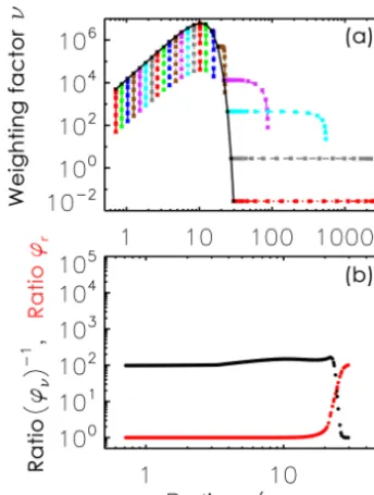
Figure 3 illustrates how AIM works for an example simu-lation with the Long kernel and singleSIP-init. The top panel shows the (ri, νi) evolution of selected SIPs. The black line shows the initial distribution. Each coloured line connects the data points that depict the (ri, νi) pair of an individual SIP every 200 s. Clearly,νiof any SIP decreases over time; how-ever, the decrease is much smaller for the largest SIPs and becomes zero for the largest SIP. The majority of SIPs start-ing from the smallest radii show an opposite behaviour, as their evolution is dominated by a strongνidecrease at nearly constantri. In contrast, the evolution of the two largest SIPs is dominated by a strongriincrease for constantνi. The SIPs next to the largest SIPs undergo a transition; in the beginning, they primarily grow in size; towards the end, the decrease of
νiis dominant.
The ratio ϕr is defined as ri(t=3600 s)/ri(t=0 s)and, analogously,ϕν=νi(t=3600 s)/νi(t=0 s). We findϕr ≥1 andϕν≤1. The bottom panel of Fig. 3 shows the ratiosϕr (red curve) and(ϕν)−1(black curve) for all SIPs of the sim-ulation. Both ratios are smooth functions of the initial ri, which is plotted on the x axis. By construction, the
num-ber of SIPs remains constant over the course of a simulation. Hence, the number of SIPs per radius or mass interval de-creases when the DSD broadens over time. In our example, the SIP resolution becomes coarser, particularly in the large droplet tail.
Negative values of νinew andχinew may occur. However,
this case never occurred in our manifold tests of the
algo-rithm. The behaviour appears more benign than in RMA. Moreover, we found that the algorithm preserved the initial size sortedness of the SIP ensemble. However, for an arbi-trary kernel function and initial SIP ensemble, this is not guaranteed, and we recommend to use adaptive sorting algo-rithms that benefit from partially presorted data sets (Estivill-Castro and Wood, 1992). Adaptive sorting is also advanta-geous when AIM is employed in real world applications, where sedimentation, advection and condensation changes the SIP ensemble in each individual grid box.
2.5 Description of the all-or-nothing algorithm (AON) The all-or-nothing algorithm (AON) is based on the ideas of Sölch and Kärcher (2010) and Shima et al. (2009). Fig-ure 2 illustrates how a collection between two SIPs is treated. SIPiis assumed to represent fewer droplets than SIPj, i.e. νi< νj. Each real droplet in SIPi collects one real droplet from SIPj . Hence, SIPicontainsνi=4 droplets, now with massµi+µj =15. SIPj now containsνj−νi=8−4=4 droplets with massµj =9. Following Eq. (23), onlyνk=2 pairs of droplets would, however, merge in reality. The idea behind this probabilistic AON is that such a collection event is realised only under certain circumstances in the model, namely such that the expectation values of collection events in the model and in the real world are the same. This is achieved if a collection event occurs with probability
Figure 3. Top: (ri, νi) evolution of selected SIPs for AIM. The
black line shows the initial distribution. Each coloured line con-nects the data points that depict the (ri, νi) pair of an
individ-ual SIP every 200 s. Bottom: the ratios ϕr and ϕν are defined
asri(t=3600 s)/ri(t=0 s)andνi(t=3600 s)/νi(t=0 s).ϕr(red
curve) and(ϕν)−1(black curve) for all SIPs are shown as a
func-tion of their initial radiusri(t=0 s). An example simulation with
Long kernel, singleSIP-init,1t=10 s, κ=40 andNSIP=197 is displayed.
in the model. Then, the average number of collections in the model,
¯
νk=pcritνi =(νk/νi)νi, (30)
is equal to νk as in the real world. A collection event be-tween two SIPs occurs ifpcrit>rand(). The function rand()
provides uniformly distributed random numbers∈ [0,1].
No-ticeably, no operation on a specific SIP pair is performed if
pcrit<rand().
The treatment of the special case νk/νi >1 needs some clarification. This case is regularly encountered when the singleSIP-init is used, where SIPs with large droplets and small νi collect small droplets from a SIP with large νj. The large difference in droplet massesµled to large kernel
values and high νk withνi < νk< νj. In addition, the case of νk being even larger thanνj is not considered, as it oc-curs only with unrealistically large time steps. If pcrit>1,
we allow multiple collections, as each droplet in SIPiis
al-lowed to collect more than one droplet from SIP j. In
to-tal, SIP i collects νk droplets from SIP j and distributes them on νi droplets. A total mass of νkµj is transferred from SIPj to SIPiand the droplet mass in SIPsibecomes µnewi =(νi µi+νk µj)/νi. The number of droplets in SIPj is reduced byνkandνjnew=νj−νk. Keeping with the
exam-ple in Fig. 2 and assumingνk=5, each of theνi=4 droplets would collectνk/νi =1.25 droplets. The properties of SIPi and SIPj are thenνi=4,µi=17.25,νj=3 andµj=9.
Another special case appears if both SIPs have the same weighting factor which regularly occurs when theνconst-init
is used. After a collection event, SIPjwould carryνj−νi= 0 droplets, whereas SIPiwould still representνidroplets. In this case, half of the droplets from SIPicoalesce with half
of the droplets from SIPj and vice versa. Accordingly, both
SIPs carryνjnew=νnewi =0.5×νi droplets with massµi+
µj. Without this correction, zero-ν SIPs would accumulate over time and reduce the effective number of SIPs, causing a poorer sampling. Instead of this equal splitting, one can also assign unequal sharesξ νiand(1−ξ )νito the two SIPs (with
ξbeing some random number).
Moreover, self-collections can be considered for kernels with Kii>0. If 2pcrit>rand(), self-collections occur be-tween the droplets in a SIP (note the factor of 2 due to sym-metry reasons). Then, every two droplets within a SIP coa-lesce, implyingνi=νi/2 andµi=2µi.
So far, we explained how a singlei−j combination is
treated in AON. In every time step, the full algorithm simply checks eachi−jcombination for a possible collection event.
To avoid double counting, only combinations withi < j and
self-collections with i=j are considered. Pseudo-code of
the algorithm is given in Algorithm (3). The SIP properties are updated on the fly. If a certain SIP is involved in a col-lection event in the model and changes its properties, all sub-sequent combinations with this SIP take into account the up-dated SIP properties. Similar to the update-on-the-fly version of RMA, results may depend on the order in which thei−j
combinations are processed.
For most i−j combinations, pcrit is small, and usually
only a limited number of collection events occurs in the model; AON may suffer from an insufficient sampling of the droplet space. Actual collections are a rare event in this algo-rithm. In our standard setup,<1% of all possible collections
occur in the model until rain is initiated by very few lucky SIPs (similar to lucky drops; e.g. Kostinski and Shaw, 2005). Indeed, Shima et al. (2009) reported convergence of AON only for tremendously many SIPs (on the order of 105to 106
in a box). We will later see that convergence is possible with as few asO(102)SIPs if the SIPs are suitably initialised.
Hence, it will be demonstrated that AON is a viable option in 2-D/3-D cloud simulations, as already implied in Arabas and Shima (2013).
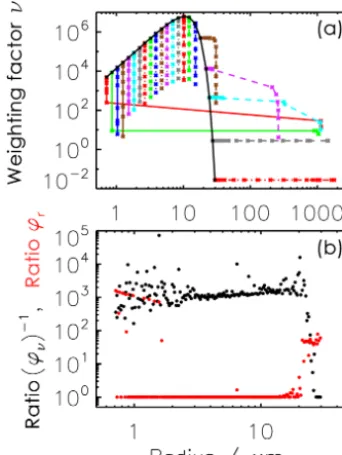
As for AIM in Fig. 3, Fig. 4 (top) shows the (ri, νi) evo-lution of selected SIPs for AON. The picture looks more chaotic than for AIM, as each individual SIP has its own in-dependent history due to the probabilistic nature of AON. For the initially smallest SIP, onlyνichanges for most of the time, as only collections occur where the partner SIPs have smaller weighting factorsν. Towards the end, the still very
Algorithm 3Pseudo-code of the all-or-nothing algorithm (AON); style conventions are explained at the end of Sect. 2.2; rand() generates uniformly distributed random numbers∈ [0,1].
1:INIT BLOCK
2:Given: Ensemble of SIPs; Specify:1t
3:TIME ITERATION
4:whilet<Tsimdo
5: {Check eachi−j-combination for a possible collection event} 6: for alli < j≤NSIPdo
7: Computeνkaccording to Eq. (19)
8: νnew=min(νi, νj) 9: pcrit=νk/νnew
10: {Update SIP properties on the fly}
11: ifpcrit>1then
12: MULTIPLE COLLECTION
13: {can occur whenνiandνjdiffer strongly and be regarded as special case; see text for further explanation}
14: assumeνi< νj, otherwise swapiandjin the following lines
15: {pcrit>1is equivalent to νk> νi}
16: {transferνkdroplets withµjfrom SIPjto SIPi, allow multiple collections in SIPi, i.e. one droplet of SIPi collects more than one droplet of SIPj.}
17: SIPicollectsνkdroplets from SIPjand distributes them onνidroplets:µi=(νiµi+νkµj)/νi
18: SIPjlosesνkdroplets to SIPi:νj=νj−νk 19: else ifpcrit>rand()then
20: RANDOM SINGLE COLLECTION
21: assumeνi< νj, otherwise swapiandjin the following lines 22: {transferνidroplets withµjfrom SIPjto SIPi}
23: SIPicollectsνidroplets from SIPj:µi=µi+µj
24: SIPjlosesνidroplets to SIPi:νj=νj−νi 25: end if
26: end for
27: t=t+1t 28:end while
29:EXTENSIONS
30:{Self-collections for a kernel withK(m, m)6=0can be treated in the following way: }
31:{Insert the following loop before line 6 or after line 26.}
32:fori=1NSIPdo 33: pcrit=νk/νi 34: if2pcrit>rand()then
35: {every two (identical) droplets coalesce}
36: νi=νi/2
37: µi=2µi
38: end if
39:end for
substantially. In contrast to the smallest SIP, other initially small SIPsiwith similar properties are never part of a
col-lection withνi < νj. Hence, their radiiri remain small over the total period, andνiis the only property that changes. The bottom panel summarises the overall changes in νi (black) andri(red) for all SIPs of the simulation. Unlike AIM, where only the initially largest SIPs grow, SIPs from both ends of
the spectrum grow in AON. Those SIPs have smallνvalues
in common, and in each collection their mass is updated to
mi+mj. The SIPs with initially largeνvalues lie in the ra-dius range[2 µm,15 µm]and keep their initial radii (at least
Figure 4.The same as Fig. 3 but for AON.
For the generation of the random numbers, the well-proven (L’Ecuyer and Simard, 2007) Mersenne Twister algorithm by Matsumoto and Nishimura (1998) is used. AON simulations may be accelerated if random numbers are computed once a priori. However, this requires saving millions of random numbers for every realisation. An AON simulation with 1000 time steps and 200 SIPs, for instance, implies 200×100 po-tential collections during 1 time step and in total 2×10⁷ ran-dom numbers. Using ranran-dom numbers with a smaller cycle length deteriorated the simulation results in several tests and is not recommended.
The current implementation differs slightly from the ver-sion in Shima et al. (2009). Due to an unfavourable SIP ini-tialisation similar to theνconsttechnique, Shima et al. (2009)
deal with largeNSIPvalues in their simulations, where it
be-comes prohibitive to evaluate all NSIP(NSIP−1)SIP
com-binations. Hence, they resort tobNSIP/2crandomly picked i−j combinations, where each SIP appears exactly in one
pair (if NSIP is odd, one SIP is ignored). As only a
sub-set of all possible combinations are numerically evaluated, the extent of collisions is underestimated. To compensate for this, the probability pcrit is upscaled with a scaling
fac-torNSIP(NSIP−1)/(2 bNSIP/2c)to guarantee an expectation
value as desired.
Moreover, in Shima’s formulation, the weighting factors are considered to be integer numbers. In contrast, we use real numbersνwhich can even attain values below 1.0. This has
several computational advantages: (1) better sampling of the DSD, in particular at the tails, (2) simpler AON implemen-tation with fewer arithmetic and rounding operations and (3)
more flexibility, e.g. SIP splitting with real-valuedξ in the
case of identical weighting factors.
The study of Sölch and Kärcher (2010) makes use of the vertical position of the SIPs and explicitly calculates whether or not a larger droplet overtakes a smaller droplet within a time step. This approach will be thoroughly analysed in a follow-up study.
In RMA and AIM, SIPs with negative weights may be gen-erated depending, e.g. on the condition1tPNSIP
j=1oij>1 in RMA. By construction, this cannot happen in AON and the latter condition implies thatPNSIP
j=1pcrit,ij of SIPiis greater than unity. Then, this SIP is likely to be involved in several collections (forj withpcrit,ij<1) or is involved in one or several multiple collections (forj withpcrit,ij>1).
3 Box model results
In this section, box model simulations of the three algorithms introduced in the latter section are presented, starting with the results of RMA, then those of AIM and finally AON. The re-sults of each algorithm are tested for three different collection kernels (Golovin, Long and Hall). As default, probabilistic SIP initialisation methods are used. For each parameter set-ting, simulations are performed for 50 different realisations. Simulations with the Golovin kernel are compared against the analytical solution given by Golovin (1963). Consistent with many previous studies, we chooseb=1.5 m3kg−1s−1.
Simulations with the Long and Hall kernels are compared against high-resolution benchmark simulations obtained by the spectral-bin model approaches of Wang et al. (2007) and Bott (1998). The volume of the box is assumed to be
1V =1 m3.
In all simulations, collision/coalescence is the only pro-cess considered in order to enable a rigorous evaluation of the algorithms. The evaluation is based on the comparison of mass density distributions and the temporal development of the zeroth, second and third moments of the droplet distribu-tions. The first moment is not shown since the mass is con-served in all algorithms per construction. The Supplement contains a large collection of figures that systematically re-port all sensitivity tests that have been performed. The be-haviour of the second and third moments is similar, and the
λ3evolution is shown only in the Supplement. Later, it will
be mentioned that Hall kernel simulations are not as chal-lenging as Long kernel simulations from a numerical point of view. Hence, simulation with the Hall kernel are only shortly discussed in the paper and figures are shown in the Supple-ment.
3.1 Performance of RMA
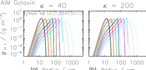
Figure 5. Mass density distributions obtained by RMA for the Golovin kernel fromt=0 to 60 min every 10 min (from black to cyan; see legend). The dotted curves show the reference solution; the solid curves show the RMA simulation results (ensemble aver-ages over 50 realisations). The parameter settings are singleSIP-init with weak thresholdη=10−8,κ=60 and1t=1 s. The follow-ing versions of RMA are depicted (clockwise from top left): regular version, version with the reduction limiter, version with update on the fly (OTFland OTFs) (starting with combinations of the largest or smallest droplets, respectively).
panel shows an excellent agreement of RMA with the ref-erence solution and proves at least a correct implementation. Figure 6 compares the temporal evolution of the moments. Moreover, the first row shows the number of SIPs used in RMA. Except for the case with a very coarse grid (κ=5)
with fewer than 40 SIPs in the end, the regular RMA results shown in the left column agree perfectly with the reference solution irrespective of the chosen κ (≥10) and minimum
weak thresholdηranging from 10−5to 10−8. The number of
non-zero bins increases as the DSD broadens over time. In the last step of the time iteration, SIPs are created from such bins. Hence, their number increases over time. Using a strict threshold, the total mass is not conserved; the largerηis, the
more mass is lost (see the Supplement). Hence, using a weak threshold or some other measure (e.g. creation of a residual SIP containing contributions of all neglected bins) to avoid this is highly recommended.
Next, RMA simulations with the Long kernel are dis-cussed. As already mentioned, the default RMA version would require tiny time steps which would rule out RMA from any practical application. Both approaches introduced before, update on the fly (OTF) and reduction limiter (RedLim), succeed in eliminating negativeνi values and in finishing the simulation within a reasonable time. However, the results are not as desired. Figure 7 shows the DSDs for a simulation with the reduction limitereγ =0.1, weak thresh-oldη=10−8, κ=20 and1t=0.1 s. Whereas the algorithm
is capable of realistically reducing the number of the smaller
Figure 6.SIP number and momentsλ0andλ2as a function of time obtained by RMA for the Golovin kernel. The black diamonds show the reference solution. The curves depict the RMA results (ensem-ble averages over 50 realisations). The default settings are proba-bilistic singleSIP-init with weak thresholdηand1t=1 s. Left col-umn: regular RMA version for variousκvalues (see legend in the middle) and thresholdη=10−8, 10−7, 10−6or 10−5(solid, dot-ted, dashed, dash-dotted; shown only forκ=40). Middle column: the same as in the left column but for the RedLim version. Right col-umn: the version with update on the fly (solid lines show OTFsand dotted lines show OTFl). The colours defineκas in the two other columns, but only the cases ofκ=10 and 60 cases are shown.
droplets, strong oscillations appear in the intermediate ra-dius range[100 µm,200 µm](see right panel). If we average
over 50 realisations (as usually, left panel) or use a coarse grain visualisation (as usually withκplot=4, middle panel),
the oscillations are smoothed out (or masked). Nevertheless, the formation of the rain mode is impeded; probably the mass flux across the problematic radius range is too slow, which is a direct consequence of applying the reduction lim-iter (mostly SIPs in this part of the spectrum obtain negative weights and have to be corrected).
We tested the algorithm for many parameter set-tings varying all of the aforementioned parameters: 1t∈ [0.01 s,1 s], κ∈ [5,100],eγ∈ [0,1] and η∈ [10−15,10−5].
Figure 8 shows the evolution of the zeroth and second mo-ments for various 1t values (at κ=10, left column) and κ values (at 1t=0.1 s right column). Obviously, the
sim-ulation results are nearly insensitive to the bin resolution (as long asκ≥10); however, the higher moment does not come
close to the reference value. The effect of a1t variation is
more substantial. Decreasing1t, the total droplet numbers
lead-Figure 7.Mass density distributions obtained by RMA for the Long kernel fromt=0 to 60 min every 10 min (from black to cyan; see legend). The dotted curves show the reference solution; the solid curves show the simulation results of RMA with the reduction lim-iter (eγ=0.1), weak thresholdη=10−
8,1t=0.1 s and κ=40. The left panel shows the average over 50 realisations and the middle panel one specific realisation. For both, the bin resolution of the vi-sualisation is by defaultκplot=4. The right panel shows again the specific realisation (onlyt=20 and 40 min) but forκplot=κ.
ing to a better agreement. Despite using already a very small time step of 0.01 s in the end (we will later see that AIM and
AON produce reasonable results for 1t=10 s), the
agree-ment with the reference solution is still not perfect.
Hence, our RMA implementation is not capable of pro-ducing reasonable results for the Long kernel. It is not clear whether the oscillations are inherent to the original RMA or caused by the introduction of the Reduction Limiter. The lat-ter might introduce discontinuities which could trigger insta-bilities.
At least, the Golovin RMA simulations with the reduction limiter do not show any signs of instability and agree well with the reference. However, this is not surprising. Clearly, the RedLim correction is only performed for SIPs, where negative weights are predicted. In Golovin simulations, this happens less frequently than in Long simulations. Only, in the very end, the abundance of the largest droplets is underes-timated (see top right panel in Fig. 5) and the increase of the higher moment levels off slightly (middle column of Fig. 6). Basically, the application of the RedLim correction, which rescales νi1, can be interpreted as an artificial reduction of
the time increment (see Eq. 20) and hence slows down the growth of all corrected SIPs.
Another RMA variant uses update on the fly, which also effectively eliminates negative weights. Such Golovin RMA simulations can be close to the reference; however, the results depend on the order in which the SIP combinations are pro-cessed. If collections between the smallest SIPs are treated first within each time iteration (OTFs), then the growth of the
largest droplets is too slow (see bottom left panel in Fig. 5). Starting the processing with collections between the largest SIPs (OTFl), the DSDs are as desired (see bottom right panel
in Fig. 5) and the moments agree perfectly with the refer-ence if κ is sufficiently large (see right column of Fig. 6).
The update on the fly has the strongest impact on those SIPs where the regular version would predict negative weights.
Figure 8.SIP number and moments λ0 and λ2 as a function of time obtained by RMA for the Long kernel. The black diamonds show the reference solution. The curves depict the RMA results (en-semble averages over 50 realisations). The default settings are the RedLim version witheγ=0.1, singleSIP-init with weak threshold η=10−8,κ=10, 1t=1 s andrcritmin=5.0 µm. The left column shows a variation of1t(see legend), the right one a variation ofκ (see legend).
With OTF, the weights of such SIPs strongly decrease dur-ing one time iteration, and hence the continuous evaluations of theOijvalues depend on the order in which the SIP com-binations are processed.
Long kernel simulations with OTFl yield results
qualita-tively similar to the RedLim version (see the Supplement) and spurious oscillations still appear in the DSDs.
Note that the Golovin simulations usedrcritmin=1.6 µm,
whereas the Long simulations used rcritmin=5.0 µm (note
the truncated left tail in the DSDs in Fig. 7). A higher
rcritminvalue reduces the SIP number and the computational
effort and made simulations with small time steps possible. The simulatedλvalues are insensitive to the choice ofrcritmin
(see the Supplement).
We conclude that, for time steps feasible in operational terms, none of the tested RMA implementations are capable of producing reasonable results with the Long kernel. An-drejczuk et al. (2010) introduced and evaluated RMA and applied it in a simulation of boundary layer stratocumulus. Our findings are seemingly in conflict with the conclusions of their evaluation exercises. What both studies have in com-mon is a similar trend for aκvariation. In their Fig. 13,
sim-ulations forκranging roughly from 4 to 30 are depicted. The