Global high-resolution simulations of tropospheric nitrogen dioxide using CHASER V4.0

(1)

https://doi.org/10.5194/gmd-11-959-2018 © Author(s) 2018. This work is distributed under the Creative Commons Attribution 4.0 License.

Global high-resolution simulations of tropospheric nitrogen dioxide

using CHASER V4.0

Takashi Sekiya1, Kazuyuki Miyazaki1,2, Koji Ogochi1, Kengo Sudo3,1, and Masayuki Takigawa1

1_{Japan Agency for Marine-Earth Science and Technology, Yokohama, Japan} 2_{Jet Propulsion Laboratory, California Institute of Technology, Pasadena, CA, USA} 3_{Graduate School of Environmental Studies, Nagoya University, Nagoya, Japan}

Correspondence:Takashi Sekiya ([email protected]) Received: 17 August 2017 – Discussion started: 9 October 2017

Revised: 18 January 2018 – Accepted: 3 February 2018 – Published: 16 March 2018

Abstract.We evaluate global tropospheric nitrogen dioxide (NO2) simulations using the CHASER V4.0 global

chemi-cal transport model (CTM) at horizontal resolutions of 0.56, 1.1, and 2.8◦. Model evaluation was conducted using satel-lite tropospheric NO2 retrievals from the Ozone

Monitor-ing Instrument (OMI) and the Global Ozone MonitorMonitor-ing Experiment-2 (GOME-2) and aircraft observations from the 2014 Front Range Air Pollution and Photochemistry Experi-ment (FRAPPÉ). AgreeExperi-ment against satellite retrievals im-proved greatly at 1.1 and 0.56◦ resolutions (compared to 2.8◦resolution) over polluted and biomass burning regions. The 1.1◦ simulation generally captured the regional distri-bution of the tropospheric NO2column well, whereas 0.56◦

resolution was necessary to improve the model performance over areas with strong local sources, with mean bias reduc-tions of 67 % over Beijing and 73 % over San Francisco in summer. Validation using aircraft observations indicated that high-resolution simulations reduced negative NO2biases

be-low 700 hPa over the Denver metropolitan area. These im-provements in high-resolution simulations were attributable to (1) closer spatial representativeness between simulations and observations and (2) better representation of large-scale concentration fields (i.e., at 2.8◦) through the consideration of small-scale processes. Model evaluations conducted at 0.5 and 2.8◦ bin grids indicated that the contributions of both these processes were comparable over most polluted regions, whereas the latter effect (2) made a larger contribution over eastern China and biomass burning areas. The evaluations presented in this paper demonstrate the potential of using a high-resolution global CTM for studying megacity-scale air

pollutants across the entire globe, potentially also contribut-ing to global satellite retrievals and chemical data assimila-tion.

1 Introduction

Nitrogen oxides (NOx∼=NO+NO2) play a key role in

air quality, tropospheric chemistry, ecosystem, and climate change. NOx is one of the main precursors of tropospheric

ozone, a major pollutant and greenhouse gas (IPCC, 2013). Oxidation products from NOx, including nitric acid (HNO3),

alkyl nitrates (RONO2), and peroxynitrates (RO2NO2), are

partitioned to particulate nitrates, which cause respiratory problems, degrade visibility, and affect the radiative budget by scattering solar radiation. The wet and dry deposition of nitrogen compounds affects the productivities and diversities of terrestrial and marine ecosystems on a global scale (e.g., Gruber and Galloway, 2008; Duce et al., 2008). Increasing NOxalso reduces quantities of long-lived greenhouse gases,

such as methane, due to chemical destruction via hydroxyl radicals (OH) through O3–HOx–NOx chemistry (e.g.,

Shin-dell et al., 2009).

Major anthropogenic sources of NOx are ground

trans-port and power generation, with these accounting for more than half of total global anthropogenic emissions (Janssens-Maenhout et al., 2015). NOx is also emitted from

natu-ral sources: biomass burning, microbial activity in soil, and lightning. Main NOx sinks are oxidation with OH during

(2)

on aerosols during nighttime (Platt et al., 1984; Dentener and Crutzen, 1993; Evans and Jacob, 2005; Brown et al., 2006). The lifetime of NOx, which is a function of OH

concentra-tion and NO2photolysis during daytime (Prather and Ehhalt,

2001), is of the order of hours to days. It also depends on aerosol surface area and composition during nighttime (e.g., Brown et al., 2006). Because of this short lifetime and het-erogeneous source distribution, tropospheric NOx is highly

variable in space and time over the globe.

Satellite observations of tropospheric NO2columns from

the Global Ozone Monitoring Experiment (GOME), the SCanning Imaging Absorption SpectroMeter for Atmo-spheric CHartographY (SCIAMACHY), the Ozone Monitor-ing Instrument (OMI) (e.g., Duncan et al., 2016; Krotkov et al., 2016), and GOME-2 (e.g., Valks et al., 2011; Zien et al., 2014) have been used for evaluations of chemical trans-port models (CTMs) (e.g., Kim et al., 2009; Huijnen et al., 2010a; Miyazaki et al., 2012; Yamaji et al., 2014). Previous model validation studies have revealed a general underes-timation of simulated tropospheric NO2columns over

pol-luted areas in global CTMs (van Noije et al., 2006; Huij-nen et al., 2010a, b; Miyazaki et al., 2012). Global CTMs typically have a horizontal resolution of 2–5◦. Meanwhile, high-resolution simulations have been conducted using re-gional models, which have shown the ability to simulate ob-served high tropospheric NO2columns over major polluted

regions such as East Asia, North America, and Europe (e.g., Uno et al., 2007; Kim et al., 2009; Huijnen et al., 2010a; Ita-hashi et al., 2014; Yamaji et al., 2014; Canty et al., 2015; Han et al., 2015; Harkey et al., 2015). High-resolution simulations can lead to improvements in two ways: (1) through reduced spatial representation gaps between observed and simulated fields and (2) via improved representation of large-scale con-centration fields through a consideration of small-scale pro-cesses. Using a regional CTM, Valin et al. (2011) suggested that insufficient model resolution leads to enhanced OH, shortened NO2 lifetime, and too-low NO2 over strong

lo-cal emissions. The authors also suggested that 4 and 12 km resolutions are sufficient to accurately simulate the nonlin-ear effects of O3–HOx–NOxchemistry on NO2lifetime over

power plants in Four Corners–San Juan and Los Angeles. Yamaji et al. (2014) estimated up to 60 % error reduction in simulated tropospheric NO2columns at 20 km resolution

over East Asia compared to 80 km resolution. Using a global CTM, Wild and Prather (2006) reported that NOx lifetime

over East Asia increased by 22 % when increasing model resolution from 5.6◦_×_5.6◦ _{to 1.1}◦_×_1.1◦_{. Williams et al.}

(2017) conducted a comprehensive evaluation of NO2, SO2,

and CH2O simulated in TM5-MP, revealing that increasing

horizontal model resolution from 3◦×2◦to 1◦×1◦reduced negative NO2bias by up to 99 % against 35 % of the surface

measurement sites (33 stations) in Europe. Horizontal model resolution could also be a crucial factor even for biomass burning areas because of highly varying emission sources and nonlinear chemical processes. However, previous studies

have mostly focused on urban regions. Further investigations are required for both urban and biomass burning regions. Ver-tical model resolution could also be important through, for instance, vertical mixing between planetary boundary layers and the free troposphere (e.g., Menut et al., 2013).

Simulated global NO2 fields provide important

informa-tion on satellite retrieval and data assimilainforma-tion, as well as contributing to a better understanding of the atmospheric en-vironment (e.g., Boersma et al., 2011; Valks et al., 2011; Miyazaki et al., 2012; Williams et al., 2017). The quality of a priori fields is important for retrieval of the tropospheric NO2

column (Russell et al., 2011). For instance, low-resolution global CTMs poorly represent NO2variations across urban

and rural regions, degrading the spatial variation of retrieved concentrations at high resolution. Several retrieval studies (Heckel et al., 2011; Russell et al., 2011; Lin et al., 2014) have employed high-resolution a priori fields from regional CTM simulations. The authors demonstrated improvements in these regional retrievals using high-resolution a priori fields in comparison to the ARCTRAS aircraft observation and ground-based remote sensing MAX-DOAS through, for instance, clearer separation of NO2profiles between urban,

rural, and ocean regions and improved representations of altitude-dependent sensitivities (i.e., averaging kernels).

Global chemical data assimilation (e.g., Inness et al., 2015; Miyazaki et al., 2015) and emission inversion (e.g., Stavrakou et al., 2013; Miyazaki et al., 2017) would also benefit from high-resolution global CTMs through improve-ments in model performance (e.g., Arellano Jr. et al., 2007) and reduced spatial representation gaps between observed and simulated fields. Several previous studies (Mijling and van der A, 2012; Ding et al., 2017b; Liu et al., 2017) demon-strated the importance of high-resolution modeling in detect-ing small-scale NOx emission sources such as urban, new

power plant, and ship emissions. A systematic evaluation of high-resolution models enables us to discuss the application potentials of global high-resolution models to satellite re-trievals and data assimilation.

In this study, we conduct a systematic evaluation of global high-resolution simulations of tropospheric NO2and related

chemistry using CHASER V4.0. We focus on the impacts of horizontal model resolution on global tropospheric NO2

sim-ulations. Three horizontal resolutions of 2.8, 1.1, and 0.56◦ are evaluated using satellite and aircraft measurements. The remainder of this paper is structured as follows. Section 2 describes the model configuration and simulation settings and optimizes the simulated meteorological fields at differ-ent horizontal resolutions. Section 2.2 describes the observa-tions used for validaobserva-tions. Section 4 presents the model eval-uation results of tropospheric NO2using satellite-derived

(3)

po-tential benefits of applying global high-resolution CTMs. Fi-nally, Sect. 7 provides concluding remarks.

2 Methodology

2.1 CHASER V4.0 model and simulations

CHASER V4.0 (Sudo et al., 2002; Sudo and Akimoto, 2007; Sekiya and Sudo, 2014) is a global chemical transport model developed in the framework of the MIROC-ESM Earth sys-tem model (Watanabe et al., 2011), which is coupled on-line with the MIROC-AGCM atmospheric general circu-lation model (AGCM) (K-1 model developers, 2004) and the SPRINTARS aerosol transport model (Takemura et al., 2005, 2009). Several updates were made from CHASER V3.0 (Sudo et al., 2002) to CHASER V4.0, which includes the consideration of aerosol species (sulfate, nitrate, ammo-nium, black and organic carbon, soil dust, and sea salt) and the implementation of related chemistry, radiation, and cloud processes. AGCM was also updated from the NIES/CCSR AGCM 5.7b to the MIROC-AGCM. Detailed information on the AGCM updates are provided by K-1 model developers (2004).

CHASER calculates gaseous, aqueous, and heterogeneous chemical reactions (93 species and 263 reactions), including the O3–HOx–NOx–CH4–CO system with the oxidation of

non-methane volatile organic compounds (NMVOCs). Ma-jor chemical reactions related to NO2are considered,

includ-ing (1) the photochemical cycle of NO and NO2, (2)

ox-idation of NO2 with OH, (3) heterogeneous hydrolysis of

N2O5, (4) the formation, thermal decomposition, and

photol-ysis of peroxyacetyl nitrates (PANs), and (5) the formation of isoprene nitrates. CHASER also calculates stratospheric O3

chemistry including Chapman mechanisms and catalytic re-actions related to HOx, NOx, ClOx, and BrOxbelow 50 hPa.

Above 50 hPa, prescribed concentrations of O3, nitrogen,

and halogen species are used. Monthly ozone climatology is obtained from UGAMP (Li and Shine, 1995), whereas monthly climatologies of nitrogen and halogen species are taken from the Chemistry–Climate Model Initiative (CCMI) REF-C1SD simulation using NIES CCM (Akiyoshi et al., 2009, 2016; Morgenstern et al., 2016). Dry and wet (rain out and washout) deposition is calculated based on the resistance-based parameterization (Wesely, 1989) and cumu-lus convection and large-scale condensation parameteriza-tions, respectively. Advective tracer transport is calculated using the piecewise parabolic method (Colella and Wood-ward, 1984) and the flux-form semi-Lagrangian scheme (Lin and Rood, 1996). The model also incorporates tracer trans-port on a sub-grid scale in the framework of the prognos-tic Arakawa–Schubert cumulus convection scheme (Emori et al., 2001) and the vertical diffusion scheme (Mellor and Yamada, 1974).

We evaluated two 1-year global simulations for tropo-spheric NO2 in 2008 and 2014 with a 1-year spin-up

culation for each simulation. In each case, three model cal-culations were conducted at different horizontal resolutions: T42 (i.e., 2.8◦×2.8◦; hereinafter referred to as the 2.8◦ sim-ulation), T106 (i.e., 1.1◦×1.1◦; hereinafter the 1.1◦ simu-lation), and T213 (i.e., 0.56◦×0.56◦; hereinafter the 0.56◦ simulation); 32 vertical layers from the surface to approxi-mately 40 km altitude were used across the three simulations. To meet the Courant–Friedrich–Levy (CFL) condition, dif-ferent maximal time steps were used for each resolution: i.e., 20 min at 2.8◦resolution, 8 min at 1.1◦resolution, and 4 min at 0.56◦resolution. Sea-surface temperatures (SSTs) and sea-ice concentrations (SICs) were prescribed by HadISST for the corresponding year (Rayner et al., 2003). Simulated air temperature and horizontal wind were nudged to 12-hourly ERA-Interim reanalysis data (Dee et al., 2011). ERA-Interim reanalysis data at 0.75◦_×_0.75◦_{horizontal resolution with 37}

pressure levels were linearly interpolated to each model grid, possibly degrading simulated meteorological fields at finer resolution (i.e., 0.56◦). We specified 5 and 0.7 days of nudg-ing time for temperature and horizontal wind, respectively.

NOx emissions from anthropogenic, biomass burning,

lightning, and soil sources were considered. Anthropogenic emissions from the HTAP_v2.2 inventory for the year 2008 (Janssens-Maenhout et al., 2015) were employed for the 2008 simulations, with these originally having 0.1◦×0.1◦ resolution. For the 2014 simulation, anthropogenic emissions for the latest available year 2010 of the HTAP_v2.2 inven-tory were used. Biomass burning emissions were taken from the Global Fire Emissions Database (GFED) version 4.1 (0.25◦_×_0.25◦ _{resolution) (Giglio et al., 2013) for the two}

study years. Soil emissions were obtained from the Global Emission InitiAtive (GEIA) database (1◦×1◦) (Yienger and Levy, 1995). Model of Emissions of Gases and Aerosols from Nature (MEGAN) version 2 data (0.5◦×0.5◦) were used for biogenic NMVOCs emissions (Guenther et al., 2006). Annual mean total global NOx emissions from the

surface were 45.3 and 45.9 Tg N yr−1in 2008 and 2014, re-spectively. Lightning NOxsources were calculated as a

func-tion of cloud top height in the cumulus convecfunc-tion parameter-ization (prognostic Arakawa–Schubert scheme) at each time step of CHASER, following Price and Rind (1992).

We considered diurnal cycles of surface NOx emissions

(4)

confirmed that the application of this scheme leads to im-provements in global tropospheric NO2 simulations at 2.8◦

resolution. Improvements were commonly found in the 1.1◦

resolution simulation, whereas we did not evaluate the im-pact at 0.56◦resolution. Over biomass burning regions, the emission diurnal variability applied in this study is generally similar to variability from 3-hourly GFED4.1 data, while dis-tinct differences in relative magnitude around the GOME-2 overpass time suggest that model performance could differ in comparison to the GOME-2 retrievals when using the 3-hourly GFED4.1 data.

The CTM–AGCM online coupling framework used in this study has advantages over the off-line CTM framework driven by meteorological analysis or reanalysis data. First, the online framework is able to simulate short-term nonlinear variations in chemical and transport processes at every time step of the model (1–20 min in this study) in contrast to off-line CTMs driven by meteorological data, typically with 6-hourly intervals. Second, grid-scale and sub-grid-scale trans-port processes (e.g., convection, turbulent mixing) are repre-sented in a consistent manner based on AGCM physics (e.g., mass balance) at short time intervals. Third, the online frame-work allows for a flexible choice of CTM resolution, whereas the off-line framework requires matching (or interpolations without physically meaningful variations) between the CTM and meteorological data resolutions.

2.2 Observations

2.2.1 Satellite tropospheric NO2retrievals

We used tropospheric NO2column retrievals from OMI and

GOME-2. OMI, onboard the Aura satellite, is an ultraviolet– visible nadir-scanning solar-backscatter spectrometer cover-ing the spectral range of 270–500 nm (Levelt et al., 2006). The Aura satellite, launched in 2004, is in a Sun-synchronous polar orbit at 705 km of altitude with a local Equator cross-ing time of approximately 13:40 LT. The ground pixel size of OMI ranges from 13×24 km2 to 26×128 km2 depend-ing on the satellite viewdepend-ing angle. OMI tropospheric NO2

column retrievals have daily global coverage. We used the DOMINO version 2.0 data product (Boersma et al., 2011) obtained from the TEMIS website (http://www.temis.nl/). Observations with cloud radiance fraction < 0.5, surface albedo<0.3, and quality flag 0 were used. Retrievals from 2014 affected by row anomalies were screened using a qual-ity flag.

Tropospheric NO2 retrievals from GOME-2 on

MetOP-A and MetOP-B were used to compare the years 2008 and 2014, respectively. GOME-2 is a nadir-scanning ultraviolet– visible spectrometer covering the spectral range of 240– 790 nm. MetOp-A, launched in 2007, and MetOp-B, launched in 2013, are on a Sun-synchronous polar orbit at 817 km with a local Equator crossing time of 09:30 LT. The ground pixel size is 80×40 km2. We used the TM4NO2A

version 2.3 product obtained from the TEMIS website (Boersma et al., 2004). The GOME-2 retrievals were de-rived with the same basic algorithm as in DOMINO version 2 (Boersma et al., 2011).

For model–retrieval comparisons, we first sampled simu-lated NO2profiles at the closest times to measurement using

2-hourly model outputs; these were then linearly interpolated to the center of each measurement from the four surrounding model grids. Second, averaging kernels (AKs) were applied to the interpolated model profiles in order to consider the altitude-dependent sensitivity of retrievals. Third, retrieved and simulated NO2columns were averaged on 0.5 and 2.8◦

bin grids for model evaluation. In order to identify the drivers of model–retrieval differences and causes of NO2 error

re-ductions in high-resolution simulations, we conducted model evaluations at 0.5 and 2.8◦bin grids (i.e., the model and re-trieval fields were interpolated to 0.5 and 2.8◦_{bin grids).}

Im-proved agreement in high-resolution simulations can be at-tributed to two factors: (1) closer spatial representativeness between simulations and satellite retrievals (up to approxi-mately 0.5◦) and (2) improvements in mean concentration fields on a large scale (i.e., at 2.8◦) through the considera-tion of small-scale processes. The error reducconsidera-tions evaluated at the 0.5◦bin grid should reflect both effects, whereas error reductions evaluated at the 2.8◦ bin grid should mainly be attributed to the latter effect (2). When error reductions eval-uated at the 2.8◦bin grid are about half the error reductions evaluated at the 0.5◦ bin grid, the contributions of the two effects should be identical. When error reductions evaluated at 2.8 and 0.5◦bin grids are comparable, the latter effect (2) should be dominant.

It should be noted that tropospheric NO2 retrievals from

SCIAMACHY were also available for 2008. The model eval-uation results are generally similar between GOME-2 and SCIAMACHY. Results using SCIAMACHY are not dis-cussed in this paper.

2.2.2 Aircraft observation data

Vertical profiles of NO, NO2, OH, HO2, O3, H2O, and

the photolysis rate of O3 to O(1D)were obtained from the

2014 Front Range Air Pollution and Photochemistry Experi-ment (FRAPPÉ) campaign (Vu et al., 2016). The FRAPPÉ campaign was conducted using the NSF/NCAR C130 air-craft during the period from 16 July through 18 August 2014. The C130 flight track covered the northern Colorado plains and foothills and the area west of the Continental Divide. NO, NO2, and O3 concentrations were measured

by two-channel (for NO and NO2) and one-channel (for

O3) chemiluminescence instruments (Ridley et al., 2004).

OH and HO2 were analyzed using a CIMS-based

instru-ment that is part of the Mauldin–Cantrell HOx CIMS

(5)

to O(1D)data, calculated from NCAR HARP–CFAS (CCD-based actinic flux spectroradiometer), were used. We used 1 min merged data obtained from the NASA LaRC Air-borne Science Data for Atmospheric Composition (http:// www-air.larc.nasa.gov/). For comparison purposes, we sam-pled simulated profiles at the closest time to measurement using 2-hourly model outputs; these were then linearly in-terpolated to measurement from the four surrounding model grids in the horizontal. The observed and simulated verti-cal profiles were compared by averaging data within each vertical pressure bin: 850 hPa (using data between the sur-face and 825 hPa), 800 hPa (825–775 hPa), 750 hPa (775– 725 hPa), 700 hPa (725–675 hPa), 650 hPa (675–625 hPa), 600 hPa (625–575 hPa), 550 hPa (575–525 hPa), and 500 hPa (525–475 hPa).

2.2.3 Ozonesonde

Simulated vertical profiles of tropospheric ozone were also evaluated using ozonesonde observations. The observed vertical profiles of ozone were obtained from the World Ozone and Ultraviolet Data Center (WOUDC, https://woudc. org/), the Southern Hemisphere ADditional OZonesondes (SHADOZ, https://tropo.gsfc.nasa.gov/shadoz/) (Thompson et al., 2003a, b), and the NOAA Earth System Research Lab-oratory (ESRL) Global Monitoring Division (GMD, https: //www.esrl.noaa.gov/gmd/). All available data from these sources were used. The observed and simulated ozone pro-files were compared at ozonesonde locations by averag-ing data within each vertical pressure bin: 850 hPa (875– 825 hPa), 500 hPa (550–450 hPa), 300 hPa (350–275 hPa), and 100 hPa (112.5–92.5 hPa).

3 Validations of meteorological fields

In the CTM-AGCM online framework, meteorological fields vary among different model resolutions. From sensitivity cal-culations, the strength and distribution of the cumulus con-vection were found to be sensitive to model resolution. The cumulus convection parameterization for 2.8◦resolution was optimized following Watanabe et al. (2011). We then at-tempted to optimize the relevant model parameters (critical relative humidity for cumulus convection and ice-fall speed) for 1.1 and 0.56◦ resolutions. The criterion was to mini-mize the root mean square error (RMSE) of annual global total flash against the Lightning Imaging Sensor (LIS), out-going longwave radiation (OLR) against the NOAA 18 satel-lite observations (Liebmann, 1996), and precipitation against the Global Precipitation Climatology Project (GPCP) (Adler et al., 2003; Huffman et al., 2009) for the year 2008. The obtained minimum values of RMSE for annual mean flash rate were 0.010, 0.011, and 0.011 flashes km−2day−1at 2.8, 1.1, and 0.56◦resolutions, respectively. Optimizing the cu-mulus convection setting reduced the positive bias of the

an-nual global mean OLR by 80 % at 1.1◦ resolution and by 50 % at 0.56◦ _{resolution. Simulated global flash frequency}

and annual global lightning NOx sources (in brackets)

var-ied slightly: 43 flashes s−1 (5.4 Tg N yr−1) at 2.8◦ resolu-tion, 47 flashes s−1 (5.6 Tg N yr−1) at 1.1◦ resolution, and 46 flashes s−1(5.5 Tg N yr−1) at 0.56◦resolution.

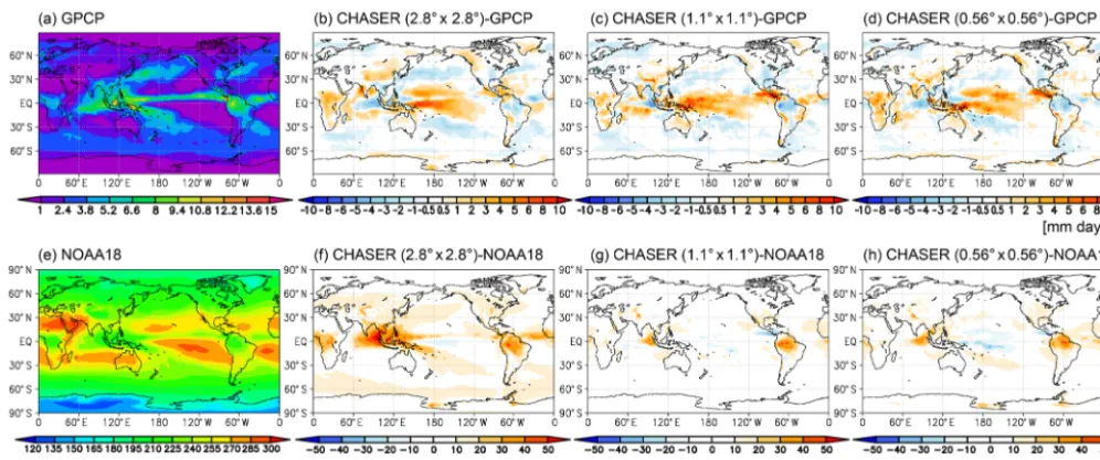
We also evaluated relevant meteorological fields (i.e., pre-cipitation and cloud) that have large impacts on chemistry simulations in the online CTM framework (e.g., Hess and Vukicevic, 2003). In comparison to the GPCP precipitation data, all simulations showed similar spatial error patterns af-ter optimization (Fig. 1a–d), having positive biases (typically by a factor of 2) north and south of the intertropical conver-gence zone (ITCZ) over the Pacific, Indian subcontinent, and Central Africa and negative biases in the South Pacific con-vergence zone (SPCZ), west of the Maritime Continent, over the Amazon, and over the southeastern United States because of the use of the same physical package (e.g., cumulus con-vection scheme). Meanwhile, increasing model resolution led to large error reductions by up to 70 % at 1.1 and 0.56◦ resolutions over the northwest Pacific and Atlantic oceans (negative biases) and over the northern part of China and the western part of the North American continent (positive biases). All simulations also showed reasonable agreement with OLR derived from the NOAA 18 satellite. The global mean positive bias was 80 and 50 % lower at 1.1 and 0.56◦ resolutions, respectively, than at 2.8◦ resolution (Fig. 1e– h), suggesting improved photolysis calculations in the high-resolution simulations. Among different regions, the positive model bias at 2.8◦ resolution was largest over the Maritime Continent, which was reduced by 86 % at 1.1◦resolution and by 75 % at 0.56◦ _{resolution. Over northern South America,}

in contrast, most of the positive biases remained at 1.1 and 0.56◦ resolutions. The model simulations were thus appro-priately set up at all resolutions, while various features of the high-resolution framework were improved. Further val-idation at various spatial–temporal scales for different me-teorological parameters will be helpful to evaluate detailed AGCM performance, even if it is beyond the scope of the current study.

4 Validations of tropospheric NO2columns and profiles

4.1 Global and regional distributions

Figure 2 compares the simulated annual mean tropospheric NO2column with satellite retrievals. Both OMI and

GOME-2 retrievals showed high tropospheric NO2 columns over

(6)

Figure 1.Annual mean precipitation rate (mm day−1) from GPCP(a)and outgoing longwave radiation (OLR; W m−2) from NOAA 18 satellite(e)for 2008. The second, third, and fourth columns show differences in precipitation(b–d)and OLR(f–h)between the observations and the model simulations at 2.8◦(b, f), 1.1◦(c, g), and 0.56◦(d, h)resolutions, respectively. The observations and model results are mapped onto 2.5 and 1◦bin grids for precipitation and OLR, respectively.

Figure 2.Annual mean tropospheric NO2 column (×1015molecules cm−2) from satellite retrievals (first column;a,e) and differences

between the model simulation at 2.8◦(second column;b,f), 1.1◦ (third column;c,g), and 0.56◦(fourth column; d, h) resolutions and satellite retrievals from OMI (upper row;a–d) and GOME-2 (lower row;e–h) for 2008. The observed and simulated fields are mapped onto a 0.5◦bin grid. The white square line in(a)represents the region used for the model evaluation.

observed global spatial variation well, withr >0.9 in com-parison to both OMI and GOME-2 for annual mean con-centration fields. In terms of global averages, the 2.8◦ sim-ulations were biased on the low side by 40 % compared to OMI and by 47 % compared to GOME-2. This negative global mean bias has commonly been reported using other global CTMs (van Noije et al., 2006; Huijnen et al., 2010b; Miyazaki et al., 2012). As summarized in Table 1, the

(7)

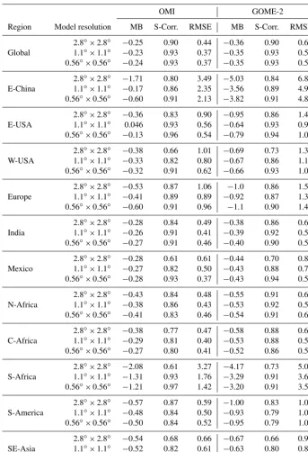
Table 1.Comparisons of annual mean tropospheric NO₂column between satellite retrievals (OMI and GOME-2) and the model simulation at 2.8, 1.1, and 0.56◦resolutions. MB is the mean bias. RMSE is the root mean square error. S-Corr. signifies the spatial correlation coefficient. Units of MB and RMSE are×1015molecules cm−2. The definition of the regions is the same as in Fig. 3.

OMI GOME-2

Region Model resolution MB S-Corr. RMSE MB S-Corr. RMSE

2.8◦×2.8◦ −0.25 0.90 0.44 −0.36 0.90 0.68 Global 1.1◦×1.1◦ −0.23 0.93 0.37 −0.35 0.93 0.58 0.56◦×0.56◦ −0.24 0.93 0.37 −0.35 0.93 0.58

2.8◦×2.8◦ −1.71 0.80 3.49 −5.03 0.84 6.89 E-China 1.1◦×1.1◦ −0.17 0.86 2.35 −3.56 0.89 4.95 0.56◦×0.56◦ −0.60 0.91 2.13 −3.82 0.91 4.87

2.8◦×2.8◦ −0.36 0.83 0.90 −0.95 0.86 1.45 E-USA 1.1◦×1.1◦ 0.046 0.93 0.56 −0.64 0.93 0.96 0.56◦×0.56◦ −0.13 0.96 0.54 −0.79 0.94 1.02

2.8◦×2.8◦ −0.38 0.66 1.01 −0.69 0.73 1.35 W-USA 1.1◦×1.1◦ −0.33 0.82 0.80 −0.67 0.86 1.18 0.56◦×0.56◦ −0.32 0.91 0.62 −0.66 0.93 1.01

2.8◦×2.8◦ −0.53 0.87 1.06 −1.0 0.86 1.54 Europe 1.1◦×1.1◦ −0.41 0.89 0.89 −0.92 0.87 1.36 0.56◦×0.56◦ −0.60 0.91 0.96 −1.1 0.90 1.48

2.8◦×2.8◦ −0.28 0.84 0.49 −0.38 0.86 0.61 India 1.1◦×1.1◦ −0.26 0.91 0.41 −0.39 0.92 0.54 0.56◦×0.56◦ −0.27 0.91 0.46 −0.40 0.90 0.57

2.8◦×2.8◦ −0.28 0.61 0.61 −0.44 0.70 0.85 Mexico 1.1◦×1.1◦ −0.27 0.82 0.50 −0.43 0.88 0.72 0.56◦×0.56◦ −0.28 0.93 0.37 −0.43 0.94 0.59

2.8◦×2.8◦ −0.43 0.84 0.48 −0.55 0.91 0.61 N-Africa 1.1◦×1.1◦ −0.38 0.86 0.43 −0.53 0.92 0.59 0.56◦×0.56◦ −0.41 0.83 0.46 −0.54 0.91 0.60

2.8◦×2.8◦ −0.38 0.77 0.47 −0.58 0.88 0.63 C-Africa 1.1◦×1.1◦ −0.29 0.81 0.40 −0.53 0.88 0.58 0.56◦×0.56◦ −0.27 0.80 0.41 −0.52 0.86 0.57

2.8◦×2.8◦ −2.08 0.61 3.27 −4.17 0.73 5.08 S-Africa 1.1◦×1.1◦ −1.31 0.93 1.76 −3.29 0.91 3.68 0.56◦×0.56◦ −1.21 0.97 1.42 −3.20 0.91 3.51

2.8◦×2.8◦ −0.57 0.87 0.59 −1.00 0.83 1.06 S-America 1.1◦×1.1◦ −0.48 0.84 0.50 −0.93 0.79 1.00 0.56◦×0.56◦ −0.50 0.84 0.52 −0.95 0.79 1.01

2.8◦×2.8◦ −0.54 0.68 0.66 −0.67 0.66 0.99 SE-Asia 1.1◦×1.1◦ −0.52 0.82 0.61 −0.63 0.80 0.89 0.56◦×0.56◦ −0.55 0.84 0.62 −0.66 0.80 0.90

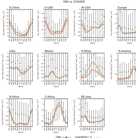
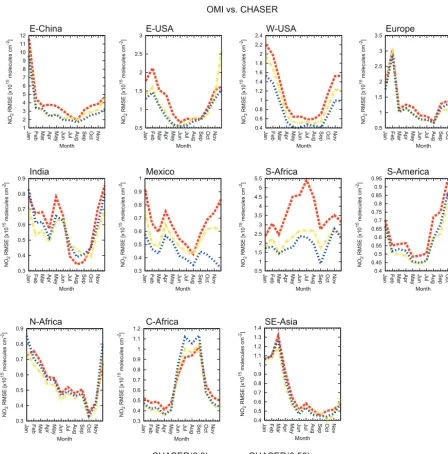
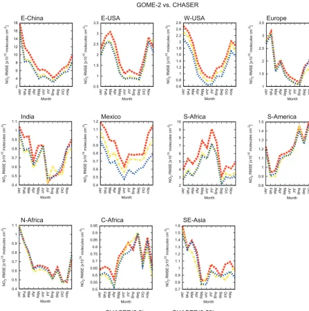
Figures 3 and 4 (5 and 6) compare seasonal variations in the regional and monthly mean tropospheric NO2 column

(regional RMSEs) against OMI and GOME-2 in 2008 using data incorporated at a 0.5◦bin grid. Because the validation results are similar for OMI and GOME-2 for most cases, the results using OMI are discussed below.

Over eastern China, negative model biases at 2.8◦ resolu-tion were reduced at 1.1 and 0.56◦_{resolutions from February}

to July. In December, model bias varied with model resolu-tion:−14 % at 2.8◦resolution,+23 % at 1.1◦resolution, and

(8)

4 6 8 10 12 14 16 18 20

Jan Feb Mar Apr May Jun Jul Aug Sep Oct Nov

T ro p. N O 2 V C D [x 10 m ol c. c m ] 15 -2 Month E-China 1.5 2 2.5 3 3.5 4 4.5 5

T ro p. N O 2 V C D [x 10 m ol c. c m ] 15 -2 Month E-USA 0.6 0.8 1 1.2 1.4 1.6 1.8 2

T ro p. N O 2 V C D [x 10 m ol c. c m ] 15 -2 Month W-USA 1 1.5 2 2.5 3 3.5 4

T ro p. N O 2 V C D [x 10 m ol c. c m ] 15 -2 Month Europe 0.6 0.8 1 1.2 1.4 1.6 1.8 2

T ro p. N O 2 V C D [x 10 m ol c. c m ] 15 -2 Month India 0.4 0.5 0.6 0.7 0.8 0.9 1 1.1 1.2

T ro p. N O 2 V C D [x 10 m ol c. c m ] 15 -2 Month Mexico 0.4 0.6 0.8 1 1.2 1.4 1.6

T ro p. N O 2 V C D [x 10 m ol c. c m ] 15 -2 Month N-Africa 0 0.5 1 1.5 2 2.5

T ro p. N O 2 V C D [x 10 m ol c. c m ] 15 -2 Month C-Africa 0 1 2 3 4 5 6

T ro p. N O 2 V C D [x 10 m ol c. c m ] 15 -2 Month S-Africa 0 0.5 1 1.5 2

T ro p. N O 2 V C D [x 10 m ol c cm ] 15 -2 Month S-America 0 0.5 1 1.5 2 2.5

T ro p. N O 2 V C D [x 10 m ol c. c m ] 15 -2 Month SE-Asia OMI vs. CHASER

OMI

CHASER(2.8) CHASER(0.56)CHASER(1.1)

Figure 3.Monthly time series of tropospheric NO₂column (×1015molecules cm−2) averaged in E-China (110–123◦E, 30–40◦N), E-USA (95–71◦W, 32–43◦N), W-USA (125–100◦W, 32–43◦N), Europe (10◦W–30◦E, 35–60◦N), India (68–88◦E, 8–35◦N), Mexico (115– 90◦W, 15–25◦N), N-Africa (20◦W–40◦E, 0–20◦N), C-Africa (10–40◦E, 20◦S–0), S-Africa (26–31◦E, 28–23◦S), S-America (70–50◦W, 20◦S–0), and SE-Asia (96–105◦E, 10–20◦N). The black dots are OMI retrievals, the red dashed line is the model simulation at 2.8◦ resolution, the yellow dashed-dotted line is the model simulation at 1.1◦resolution, and the blue dotted line is the model simulation at 0.56◦ resolution. The vertical bars indicate mean OMI retrieval errors.

(fromr=0.80 at 2.8◦resolution tor=0.86 at 1.1◦ resolu-tion and 0.91 at 0.56◦_{resolution). Annual mean RMSE was}

also reduced by 32 % from 2.8 to 1.1◦_{resolution and by 9 %}

from 1.1 to 0.56◦resolution.

Over the eastern United States, negative annual mean bias was reduced by 87 % at 1.1◦resolution and by 65 % at 0.56◦ resolution compared to 2.8◦resolution. The seasonal bias re-duction reached 95 % at 0.56◦resolution in summer. Annual

RMSE was reduced by 37 % at 1.1◦resolution and by 40 % at 0.56◦_{resolution compared to 2.8}◦_{resolution. The larger}

monthly RMSE at 1.1◦ _{than at 2.8}◦ _{resolution during}

(9)

E-China E-USA W-USA Europe

India Mexico

N-Africa C-Africa

S-Africa S-America

SE-Asia GOME-2 vs. CHASER

5 10 15 20 25

T ro p. N O 2 V C D [x 10 m ol c. c m ] 15 -2 Month 2 2.5 3 3.5 4 4.5 5 5.5 6

T ro p. N O 2 V C D [x 10 m ol c. c m ] 15 -2 Month 0.5 1 1.5 2 2.5

T ro p. N O 2 V C D [x 10 m ol c. c m ] 15 -2 Month 1.5 2 2.5 3 3.5 4

T ro p. N O 2 V C D [x 10 m ol c. c m ] 15 -2 Month 0.6 0.8 1 1.2 1.4 1.6 1.8 2

T ro p. N O 2 V C D [x 10 m ol c. c m ] 15 -2 Month 0.6 0.8 1 1.2 1.4

T ro p. N O 2 V C D [x 10 m ol c. c m ] 15 -2 Month 0 2 4 6 8 10

T ro p. N O 2 V C D [x 10 m ol c. c m ] 15 -2 Month 0 0.5 1 1.5 2 2.5

T ro p. N O 2 V C D [x 10 m ol c. c m ] 15 -2 Month 0.4 0.6 0.8 1 1.2 1.4

T ro p. N O 2 V C D [x 10 m ol c. c m ] 15 -2 Month GOME-2

CHASER(2.8) CHASER(0.56)CHASER(1.1)

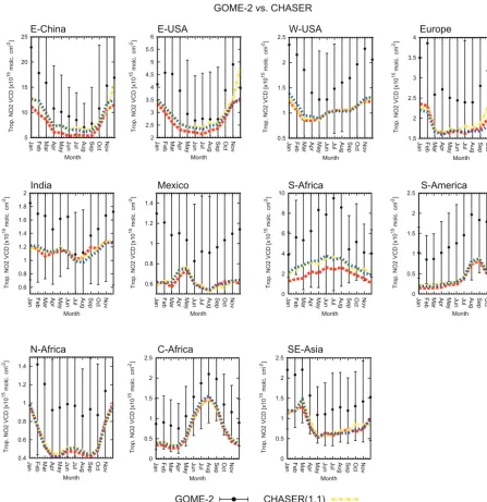
Figure 4.Same as Fig. 3, but for GOME-2.

Over the western United States, negative annual mean bias was 13 % lower at 1.1◦resolution and 14 % lower at 0.56◦ resolution compared to 2.8◦resolution. In summer, the neg-ative seasonal mean bias at 0.56◦ resolution was slightly larger, reflecting negative biases over rural areas. RMSE for annual mean fields was reduced by 20 % from 2.8 to 1.1◦ res-olution and by 23 % from 1.1 to 0.56◦resolution. The spatial correlation for annual mean fields increased from r=0.65 at 2.8◦_{resolution to}_r₌₀_._{82 at 1.1}◦_{resolution and 0.91 at}

0.56◦_resolution.

Over Europe, negative model bias for annual mean con-centrations was reduced by 23 % from 2.8 to 1.1◦resolution,

but was 46 % larger at 0.56◦ resolution than at 1.1◦ resolu-tion. Large negative bias over the Po Valley at 2.8◦resolution was reduced by 13 % at 1.1◦resolution and further reduced by 10 % from 1.1 to 0.56◦resolution. In contrast, negative bias over London was larger at 0.56◦resolution than at 1.1◦ resolution by a factor of 4, leading to larger negative regional mean bias at 0.56◦resolution. Simulated planetary boundary layer (PBL) height in the 0.56◦simulation was substantially higher (by 20 %) than ERA-Interim over London, which may partially contribute to the large NO2bias. Annual RMSE was

(10)

India Mexico

N-Africa C-Africa

S-Africa S-America

SE-Asia OMI vs. CHASER

CHASER(2.8) CHASER(1.1) CHASER(0.56) 1 2 3 4 5 6 7 8 9 10 11 12

NO

2

RMSE [x10

15 molecules cm -2] Month 0.5 1 1.5 2 2.5 3

NO

2

RMSE [x10

15 molecules cm -2] Month 0.4 0.6 0.8 1 1.2 1.4 1.6 1.8 2 2.2 2.4

NO

2

RMSE [x10

15 molecules cm -2] Month 0.5 1 1.5 2 2.5 3 3.5

NO

2

RMSE [x10

15 molecules cm -2] Month 0.3 0.4 0.5 0.6 0.7 0.8 0.9

NO

2

RMSE [x10

15 molecules cm -2] Month 0.3 0.4 0.5 0.6 0.7 0.8 0.9 1

NO

2

RMSE [x10

15 molecules cm -2] Month 0.5 1 1.5 2 2.5 3 3.5 4 4.5 5 5.5

NO

2

RMSE [x10

15 molecules cm -2] Month 0.4 0.45 0.5 0.55 0.6 0.65 0.7 0.75 0.8 0.85 0.9 0.95

NO

2

RMSE [x10

15 molecules cm -2] Month 0.3 0.4 0.5 0.6 0.7 0.8 0.9

NO

2

RMSE [x10

15 molecules cm -2] Month 0.3 0.4 0.5 0.6 0.7 0.8 0.9 1 1.1 1.2

NO

2

RMSE [x10

15 molecules cm -2] Month 0.4 0.5 0.6 0.7 0.8 0.9 1 1.1 1.2 1.3 1.4

NO

2

RMSE [x10

15 molecules cm -2]

Month

Figure 5.Same as Fig. 3, but for root mean square error (RMSE) of tropospheric NO2column in comparison to OMI.

annual mean fields increased from 0.87 at 2.8◦resolution to 0.91 at 0.56◦_resolution.

Over India, negative model biases were smaller at 1.1 and 0.56◦ resolutions than at 2.8◦ resolution during January– May, but were larger during June–September. RMSE for an-nual mean fields was reduced at 1.1 and 0.56◦ resolutions (except during summer), with 16 and 6 % reductions, respec-tively. When comparing against OLR and precipitation ob-servations, we found an increased error at 0.56◦ resolution over India during summer. This suggests the need to further optimize model parameters relevant to tropical convection

(see Sect. 2) in order to improve high-resolution NO2

sim-ulations.

Over Mexico, the spatial correlation for annual mean fields increased substantially at 1.1◦(r=0.82) and 0.56◦ resolu-tions (r=0.93) compared to 2.8◦resolution (r=0.61). In-creasing model resolution was important to reduce negative biases around Mexico City, reducing annual RMSE by 17 % at 1.1◦resolution and by 38 % at 0.56◦resolution compared to 2.8◦resolution.

(11)

India Mexico

N-Africa C-Africa

S-Africa S-America

SE-Asia GOME-2 vs. CHASER

CHASER(2.8) CHASER(1.1) CHASER(0.56) 2 4 6 8 10 12 14 16 18

NO

2

RMSE [x10

15 molecules cm -2] Month 0.5 1 1.5 2 2.5 3 3.5

NO

2

RMSE [x10

15 molecules cm -2] Month 0.6 0.8 1 1.2 1.4 1.6 1.8 2 2.2 2.4 2.6

NO

2

RMSE [x10

15 molecules cm -2] Month 1 1.5 2 2.5 3 3.5

NO

2

RMSE [x10

15 molecules cm -2] Month 0.4 0.5 0.6 0.7 0.8 0.9 1 1.1

NO

2

RMSE [x10

15 molecules cm -2] Month 0.4 0.5 0.6 0.7 0.8 0.9 1 1.1 1.2

NO

2

RMSE [x10

15 molecules cm -2] Month 2 3 4 5 6 7 8 9 10

NO

2

RMSE [x10

15 molecules cm -2] Month 0.8 0.9 1 1.1 1.2 1.3 1.4 1.5

NO

2

RMSE [x10

15 molecules cm -2] Month 0.4 0.5 0.6 0.7 0.8 0.9 1 1.1

NO

2

RMSE [x10

15 molecules cm -2] Month 0.5 0.55 0.6 0.65 0.7 0.75 0.8 0.85 0.9 0.95

NO

2

RMSE [x10

15 molecules cm -2] Month 0.7 0.8 0.9 1 1.1 1.2 1.3 1.4 1.5 1.6

NO

2

RMSE [x10

15 molecules cm -2]

Month

Figure 6.Same as Fig. 3, but for RMSE of tropospheric NO2column in comparison to GOME-2.

reduced by 46 and 56 % at 1.1 and 0.56◦_resolutions,

respec-tively. The spatial correlation was 0.93 and 0.97 at 0.56◦

resolution in contrast to 0.61 at 2.8◦resolution. Model res-olution higher than 1.1◦ was thus important for reproduc-ing megacity-scale air pollution over the Highveld region of South Africa, which is a complex source area of coal mining, thermal power generation, metal mining, and metallurgical industry as discussed by Duncan et al. (2016).

Over the selected biomass burning regions (South Amer-ica, North AfrAmer-ica, Central AfrAmer-ica, and Southeast Asia), all model simulations showed negative biases throughout the year. In most cases, bias reduction with increasing model

(12)

bias was reduced by 24 % at 1.1◦resolution and by 30 % at 0.56◦_{resolution, while RMSE increased during the biomass}

burning season (by 11 % at 1.1◦ _{resolution and by 24 % at}

0.56◦ resolution). The increased RMSE is associated with increased positive biases around 10–20◦S. Over Southeast Asia, RMSE for the annual mean fields was reduced by 7 % at 1.1◦resolution and by 5 % at 0.56◦resolution compared to 2.8◦resolution. The increased errors over strong biomass burning hot spots in high-resolution simulations could be a result of more pronounced influences of largely uncertain inventories for individual burning points (e.g., Castellanos et al., 2015).

Negative biases with respect to GOME-2 were larger than to OMI in all simulations over most regions. The differences suggest that all model simulations underestimated high NO2

concentrations in the morning. The underestimations could be associated with insufficient vertical model resolution for capturing thin nocturnal boundary layers and uncertainties in HOx–NOx–CO–VOCs chemistry, NO2photolysis rates, and

emission diurnal cycles. The different model biases between OMI and GOME-2 could also be attributed to the bias be-tween these retrievals. Irie et al. (2012) concluded that the bias between these retrievals is small and insignificant for East Asia, whereas the bias between these retrievals is un-clear for other regions. For the most anthropogenically pol-luted regions, bias reductions at 0.56◦(compared to 2.8◦ res-olution) were similarly found for OMI and GOME-2. For South America and Central Africa, reductions of the nega-tive bias at 0.56◦ resolution were larger in the comparison against OMI than GOME-2 during the biomass burning sea-son, suggesting that the high-resolution simulation improves the representation of daytime photochemistry in the presence of enhanced biomass burning emissions.

For the evaluations, we used simulated and observed con-centrations interpolated to a 0.5◦ bin grid. To identify the main drivers of improvements in the high-resolution sim-ulation, we conducted further comparisons using two con-centration fields interpolated to 2.8 and 0.5◦bin grids. The drivers consist of (1) closer spatial representativeness be-tween observations and simulations (up to approximately 0.5◦ resolution) and (2) better representation of large-scale (i.e., at 2.8◦) concentration fields through the considera-tion of small-scale processes. Error reducconsidera-tions at the 0.5◦ bin grid include the effects of both drivers. In contrast, er-ror reductions at the 2.8◦ bin grid are mainly attributed to the latter effect (2). When error reductions at the 2.8◦ bin grid are about half those at the 0.5◦ _{bin grid, the}

contri-butions of the two effects should be identical. For annual RMSE reductions, the contributions of the two effects were almost identical over the eastern United States, the west-ern United States, and South Africa (by up to −1.9 and

−0.9×1015molecules cm−2 at 0.5 and 2.8◦ bin grids, re-spectively). In contrast, over eastern China, improved rep-resentations on the large scale (2) contributed up to 90 % (i.e., reductions by 1.1 and 1.0×1015molecules cm−2at 0.5

and 2.8◦bin grids, respectively, at 1.1◦resolution). In this re-gion, the large contribution of the second effect reflected spa-tially homogeneous error reductions over Hebei and Henan provinces. Over most biomass burning areas, improved rep-resentations on the large scale (2) dominated improvements in high-resolution modeling, with RMSE reductions of up to 0.072×1015molecules cm−2 for the 2.8◦ bin grid and 0.071×1015molecules cm−2for the 0.5◦bin grid. These re-sults imply that, even for areas with homogeneous concentra-tion and emission fields, high-resoluconcentra-tion modeling can have significant impacts through a better representation of large-scale fields.

4.2 Tropospheric NO2over strong local sources

Figure 7 compares the detailed spatial distribution of the tropospheric NO2 column in summer, as represented by

OMI measurements and model simulations over four selected polluted areas: East Asia, South Asia, the western United States, and South Africa. Over East Asia, high concentra-tions were observed over the North China Plain, the Yangtze River Delta, the Pearl River Delta, Seoul, and Tokyo, which could mainly be attributed to emissions from traffic (Zheng et al., 2014) and large coal-fired power plants in the North China Plain (Liu et al., 2015). The 2.8◦ simulation under-estimated these high concentrations and overunder-estimated low concentrations over surrounding areas, probably associated with artificial mixing at coarse model resolution. The 1.1 and 0.56◦ simulations reduced negative biases over central eastern China, the Pearl River Delta, Seoul, Tokyo, and the western part of Japan. Over the Yellow Sea, the East China Sea, and off the Pacific coast of Japan, the positive biases at 2.8◦ _{resolution were mostly removed at 1.1 and 0.56}◦

res-olutions. Consequently, regional RMSE was 32 % lower at 0.56◦resolution. In contrast, high-resolution simulations led to overestimation over Beijing and the Yangtze River Delta.

Over South Asia, high concentrations were observed over large cities such as New Delhi, Chennai, Mumbai, and Kolkata in India, over Lahore and Multan in Pakistan, and around reported coal-based thermal power plants at 24◦N, 83◦E and 22◦N, 83◦E in India (Lu and Streets, 2012; Prasad et al., 2012). The 2.8◦simulation was biased on the low side by up to 50 % over these areas, except westward of New Delhi, as commonly reported using another coarse-resolution model at 2.8◦ resolution (Sheel et al., 2010). These nega-tive biases were reduced by up to 50 % at 1.1 and 0.56◦ res-olutions, whereas high-resolution simulations reveal exces-sively high concentrations over New Delhi. Over rural areas, negative biases were larger at 1.1 and 0.56◦ resolutions, re-sulting in larger regional RMSE than at 2.8◦resolution (see Sect. 4.1).

(13)

(a) OMI (b) CHASER (2.8° x 2.8°) - OMI (c) CHASER (1.1° x 1.1°) - OMI (d) CHASER (0.56° x 0.56°) - OMI

(e) OMI (f) CHASER (2.8° x 2.8°) - OMI (g) CHASER (1.1° x 1.1°) - OMI (h) CHASER (0.56° x 0.56°) - OMI

(i) OMI (j) CHASER (2.8° x 2.8°) - OMI (k) CHASER (1.1° x 1.1°) - OMI (l) CHASER (0.56° x 0.56°) - OMI

(m) OMI (n) CHASER (2.8° x 2.8°) - OMI (o) CHASER (1.1° x 1.1°) - OMI (p) CHASER (1.1° x 1.1°) - OMI

[x1015_{molecules cm}-2_]

MB = -0.11

RMSE = 0.90 RMSE = 0.72MB = -0.09 RMSE = 0.61MB = -0.11

MB = -0.22

RMSE = 0.36 MB = -0.25RMSE = 0.40 MB = -0.27RMSE = 0.39

MB = -0.16

MB = -0.48

Beijing

Tianjin Shanghai

Nanjing

Shenzhen Guangzhou

Seoul Tokyo

Lahore

New Delhi

Kolkata

Chennai Mumbai Multar

Los Angeles San Francisco Seattle

Phoenix Salt Lake City

Denver

Four Corners

[x1015_{molecules cm}-2_]

Figure 7.Tropospheric NO2column (×1015molecules cm−2) from OMI retrievals (first column;a,e,i,m) and differences between the

model simulation at 2.8◦(second column;b,f,j,n), 1.1◦(third column;c,g,k,o), and 0.56◦(fourth column;d,h,l,p) resolutions and OMI retrievals over East Asia (first row;a–d), South Asia (second row;e–h), and the western United States (third row;i–l) during JJA and over South Africa (forth row;m–p) during DJF 2008. Observed and simulated fields are mapped onto a 0.5◦bin grid. Regional mean bias (MB) and RMSE are also shown.

increasing model resolution over most of these regions. In contrast, negative biases remained at 0.56◦resolution around strong local sources. Over rural areas, negative biases in-creased with model resolution, partly reflecting suppressed artificial dilution from strong local sources. As a result, re-gional RMSE was reduced by 18 and 27 % at 1.1 and 0.56◦ resolutions compared to 2.8◦resolution. Errors, for instance, in soil NOxemissions in summer (e.g., Oikawa et al., 2015;

Weber et al., 2015) could contribute to underestimations over rural areas.

(14)

0 5 10 15 20 25 30

M

od

el

[x

10

m

ol

c.

c

m

]

15

-2

Observation [x10 molc. cm ]15 -2

0 2 4 6 8 10 12

M

od

el

[x

10

m

ol

c.

c

m

]

15

-2

Observation [x10 molc. cm ]15 -2 OMI vs. CHASER

(a) East Asia (b) The western US

GOME-2 vs. CHASER

0 5 10 15 20 25 30 35 40

M

od

el

[x

10

m

ol

c.

c

m

]

15

-2

Observation [x10 molc. cm ]15 -2 (c) East Asia

0 2 4 6 8 10 12 14

M

od

el

[x

10

m

ol

c.

c

m

]

15

-2

Observation [x10 molc. cm ]15 -2 (d) The western US

Slope = -0.19, 0.040, 0.67

Intercept = 6.4, 7.1, 2.8 r = -0.31, 0.040, 0.36

Slope = 0.15, 0.24, 0.31

Intercept = 0.64, 0.99, 1.6 r = 0.95, 0.95, 0.94

Slope = -0.31, -0.16, -0.38

Intercept = 11.9, 13.2, 21.9 r = -0.58, -0.19, 0.44

Slope = 0.14, 0.22, 0.40

Intercept = 0.66, 1.0, 1.5 r = 0.92, 0.92, 0.94

Figure 8.Scatter plots of observed and simulated tropospheric NO2column (×1015molecules cm−2) over strong local sources in East

Asia (left column;a,c) and the western United States (right column;b,d) during JJA 2008 for the OMI retrievals (upper row;a–b) and GOME-2 retrievals (lower row;c–d). The red marks are the model simulation at 2.8◦resolution, the yellow marks are the model simulation at 1.1◦resolution, and the blue marks are the model simulation at 0.56◦resolution. The horizontal bars indicate mean retrieval errors in OMI and GOME-2. For East Asia, the results are shown for Beijing (116.38◦E, 39.92◦N), Tianjin (117.18◦E, 39.13◦N), Shanghai (121.47◦E, 31.23◦N), Nanjing (118.77◦E, 32.05◦N), Guangzhou (113.27◦E, 23.13◦N), Shenzhen (114.10◦E, 22.55◦N), Seoul (126.96◦E, 37.57◦N), and Tokyo (139.68◦E, 35.68◦N). For the western United States, the results are shown for Los Angeles (118.25◦W, 34.05◦N), San Fran-cisco (122.42◦W, 37.78◦N), Seattle (122.33◦W, 47.61◦N), Salt Lake City (111.88◦E, 40.75◦N), Phoenix (112.07◦W, 33.45◦N), Denver (104.88◦W, 39.76◦N), and the Four Corners and San Juan power plants (108.48◦W, 36.69◦N). The values and mean retrieval errors are averages within a 50 km distance from each strong source, with weighting function application based on the inverse of the distance from each location.

Negative bias (75 % at 2.8◦resolution) in the Johannesburg– Pretoria megacity area (28◦E, 25.7–26.2◦S) was also re-duced to 54 % at 1.1◦resolution and 50 % at 0.56◦resolution. High-resolution simulations are thus important for regions with complex and strong local sources. At the same time, the remaining negative bias at 0.56◦ suggests that power plant and industrial emissions are underestimated, as suggested by

Miyazaki et al. (2017), or that a model resolution higher than 0.56◦is essential.

Figure 8 compares simulated high NO2 concentrations

(15)

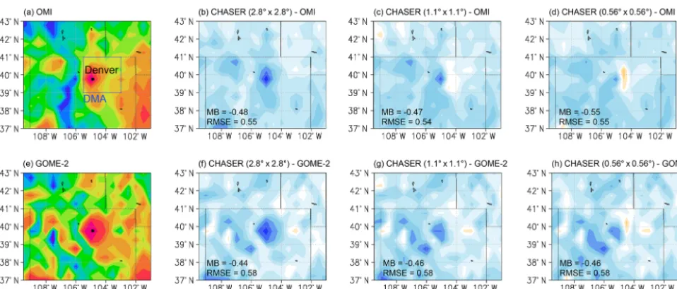
evalu-Figure 9.Regional distributions of tropospheric NO2column (×1015molecules cm−2) from satellite retrievals (first column;a,e) and

differences between the model simulation at 2.8◦(second column;b,f), 1.1◦(third column;c,g), and 0.56◦(fourth column;d,h) resolutions and satellite retrievals from OMI (upper row; a–d) and GOME-2 (lower row; e–h) over Colorado state during July–August 2014. The observed and simulated fields are mapped onto a 0.5◦bin grid. The DMA area is shown by the blue square in(a).

ating local NO2pollution because of the short NO2lifetime.

For the comparisons, retrieved and simulated tropospheric NO2 columns were averaged within a 50 km distance from

the selected points while applying a distance-based weight-ing function (i.e., the inverse of the distance was applied to each retrieval).

In comparison to OMI retrievals, with increasing model resolution, the slope for East Asia became closer to 1 (0.67 at 0.56◦resolution and−0.19 at 2.8◦resolution), and the inter-cept number became smaller (2.8 at 0.56◦resolution and 6.4 at 2.8◦resolution). The correlation coefficient also increased (r=0.36 at 0.56◦resolution in contrast tor= −0.31 at 2.8◦ resolution). Large negative biases were reduced at 0.56◦ res-olution by 67 % over Beijing, by 73 % over Tianjin, by 18 % Shanghai, by 90 % over Nanjing, by 62 % over Guangzhou, by 48 % over Shenzhen, by 47 % over Seoul, and by 62 % over Tokyo (compared to 2.8◦resolution). The estimated bi-ases at 0.56◦ resolution are within mean OMI retrieval er-rors. Reductions in negative biases at 0.56◦resolution against GOME-2 were also observed: by 91 % over Beijing, by 70 % over Tianjin, by 76 % over Shanghai, by 67 % over Nan-jing, by 32 % over Guangzhou, by 50 % over Shenzhen, by 40 % over Seoul, and by 58 % over Tokyo. However, there is more degradation of slope and intercept against GOME-2 than against OMI, reflecting large negative biases over Guangzhou, Shenzhen, Seoul, and Tokyo.

Over the western United States, NO2columns in all model

simulations were in agreement with OMI retrievals (r >0.9). The 0.56◦ model reduced negative biases with respect to OMI by 30 % over Los Angeles, by 74 % over San Francisco,

by 98 % over Seattle, by 58 % over Salt Lake City, by 83 % over Phoenix, by 44 % over Denver, and by 78 % over the Four Corners and San Juan power plants (compared to the 2.8◦ model). These bias reductions resulted in an improved slope number at 0.56◦resolution (0.31) compared to 2.8◦ res-olution (0.15). In this region, comparison results were gen-erally similar between OMI and GOME-2. These validation results demonstrate the capability of the 0.56◦_{simulation to}

represent high concentrations over strong local sources.

4.3 Validations using FRAPPÉ aircraft measurements

In this section, we evaluated model performance in relation to O3–HOx–NOx chemistry over the Denver metropolitan

area (DMA; defined as 39–41◦N and 103–105.5◦W) in the western United States using the FRAPPÉ campaign obser-vation data and satellite retrievals from July–August 2014. Figure 9 compares the spatial distribution of the tropospheric NO2 columns between simulations and satellite retrievals

around the FRAPPÉ locations. OMI and GOME-2 observed high tropospheric NO2 columns over the DMA at around

40◦_{N, 105}◦_{W. All models underestimated high}

concentra-tions by about 50 % at 2.8◦ _{resolution compared to OMI,}

(16)

Observation

CHASER (2.8) CHASER (0.56)CHASER (1.1) (b) NO₂

(a) NO (c) NO₂ 09:00–12:00 LT (d) NO₂ 13:00–16:00 LT

(e) OH (f) HO₂ (g) O3 (h) H2O

(i) J(O3→O¹D) (j) O(¹D)+H2O→2OH

500

700

800

900 0 100 200 300 400 500 600 700 800

Pressure

NO [pptv]

500

700

800

900 0 500 1000 1500 2000

NO₂ [pptv]

500

700

800

900 0 1000 2000 3000 4000 5000

NO₂ [pptv]

500

700

800

900₀ ₂₀₀ ₄₀₀ ₆₀₀ ₈₀₀ ₁₀₀₀

NO₂ [pptv]

500

700

800

900 0.05 0.1 0.15 0.2 0.25 0.3 0.35 0.4 0.45 0.5

Pressure

OH [pptv]

500

700

800

900 10 15 20 25 30 35 40 HO₂ [pptv]

500

700

800

900 40 45 50 55 60 65 70 75 80 O₃ [ppbv]

500

700

800

900 4 6 8 10 12 14 16 H O [g kg₂ -1]

500

700

800

900 1e-05 2e-05 3e-05 4e-05 5e-05 6e-05

Pressure

J1 [1/s]

500

700

800

900 1e+07 2e+07 3e+07 4e+07 5e+07 6e+07

P(HO ) from O D+H O [molecules cm-3_s-1_]

x 1 2

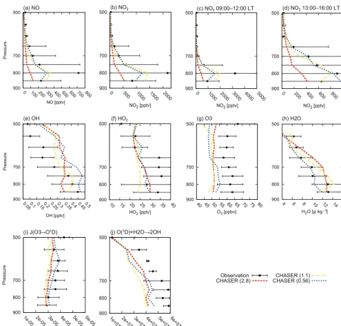
Figure 10. Vertical profiles of NO (pptv) (a), NO2 (pptv) (b), NO2 during mornings (09:00–12:00 LT) (c) and afternoons (13:00–

16:00 LT)(d), OH (pptv)(e), HO2(pptv)(f), O3(ppbv)(g), specific humidity (g kg−1)(h), the photolysis rate of O3(s−1)(i), and the OH

chemical production rate (molecules cm−3s−1) from O1D and H2O(j)over the Denver metropolitan area (39–41◦N and 103–105.5◦W)

during the FRAPPÉ period (from 16 July to 18 August 2014). The black dots represent the measurements, the red dashed line is the model simulation at 2.8◦resolution, the yellow dashed-dotted line is the model simulation at 1.1◦resolution, and the blue dotted line is the model simulation at 0.56◦resolution. The horizontal bars represent the standard deviation of the measurements.

and GOME-2 for the entire domain area was almost constant with varying model resolution.

Figure 10 compares mean vertical profiles of trace gases and reaction rates over the DMA. Large negative biases of NO and NO2at 2.8◦resolution were mostly removed at 1.1

and 0.56◦ resolutions below 650 hPa (by up to 88 %), ex-cept at 800 hPa during daytime (09:00–16:00 LT). All

(17)

0.1 0.2 0.3 0.4 0.5 0.6

100 1000 10 000

OH [pptv]

NO [pptv] (b) OH

5 10 15 20 25 30 35 40

100 1000 10 000

HO

2

[pptv]

NO [pptv] (c) HO2

Observation

CHASER (2.8) CHASER (0.56)CHASER (1.1)

(a) NO probability distribution function

0 0.1 0.2 0.3 0.4 0.5

100 1000 10 000

Probability

NO [pptv]

Figure 11. (a)Probability distribution functions of NO,(b)OH, and(c)HO2as a function of NO (pptv). The black dots represent

measure-ments, the red dashed line is the model simulation at 2.8◦resolution, the yellow dashed-dotted line is the model simulation at 1.1◦resolution, and the blue dotted line is the model simulation at 0.56◦resolution. The vertical bars represent the standard deviation of the measurements.

48 % at 1.1◦_{resolution, and by 62 % at 2.8}◦_{resolution. The}

remaining large bias in the morning at 0.56◦_{resolution could}

be associated with insufficient vertical model resolution to represent mixing within nocturnal thin boundary layers.

Large negative OH biases at 2.8 and 1.1◦ resolutions at 850 hPa were reduced by 81 % at 0.56◦resolution. From 800 to 750 hPa, the 1.1◦simulation showed the closest agreement with observations (0.5–7 %), whereas the 2.8 and 0.56◦ simu-lations underestimated OH by 7–21 % and overestimated OH by up to 27 %, respectively. Above 700 hPa, all simulations overestimated OH with a factor of up to 2. All simulations also underestimated HO2by 10–32 % below 650 hPa, except

at 800 hPa.

OH and HO2concentrations depend greatly on NOx

con-centrations through O3–HOx–NOx chemistry, as well as

HOx production and OH conversion reactions to peroxy

radicals (HO2 and RO2) with CO and VOCs. Figure 11a

shows the probability distribution function of NO from the FRAPPÉ aircraft observation and the model simulations at 800 hPa over the DMA. The observation revealed a wide range of NO concentrations from 10–10 000 pptv. The 2.8◦ simulation overestimated the occurrence of concentrations

<100 pptv and underestimated the occurrence of concen-trations>100 pptv. The 1.1 and 0.56◦simulations captured the observed probability distribution function, although they slightly overestimated the peak frequency concentration and underestimated the occurrence of low (<100 pptv) and high (>1000 pptv) concentrations. Figure 11b shows the OH– NO relationship used to validate O3–HOx–NOx chemistry.

The observation showed OH increase with increasing NO to 350 pptv and a decrease with increasing NO from 350 pptv; all simulations captured the lower part (NO<800 pptv) of the observed NO–OH relationship, suggesting that the model realistically simulates nonlinear O3–HOx–NOx chemistry.

The lack of high NO (>800 pptv) with low OH resulted in an overestimation of mean OH concentrations at 0.56◦ reso-lution.

Figure 11c compares the HO2–NO relationship. All

simulations underestimated the occurrence of high HO2

(>25 pptv) at low NO (<100 pptv). This implies an under-estimation of HOx chemical production in the simulations.

We evaluated HOxproduction from the chemical reaction of

O(1D) with H2O using temperature, specific humidity, O3

photolysis rate to O(1D)(J_O

3→O(1D)), and O3concentration

with the assumption of O(1D)equilibrium (Fig. 10g–j). All simulations underestimated HOx production, with the

un-derestimation being smaller by 13 % at 0.56◦ _{resolution at}

800 hPa. The underestimation of HOx production was

pri-marily attributable to a negative bias in O3 by 11 % and

J_O

3→O(1D)by 2.5 % at 0.56

◦_{resolution at 800 hPa. The}

neg-ative biases of O3 and JO3→O(1D) were reduced by 39 and

58 %, respectively, at 0.56◦ (compared to 2.8◦) resolution. Biases in specific humidity also had small impacts on cal-culated HOx production. Positive biases of specific

humid-ity at 2.8◦resolution above 750 hPa were reduced by up to 83 % at 0.56◦resolution. The lack of nitrous acid (HONO) in the model could explain a component of the HOxproduction

underestimation, especially during mornings (e.g., Kanaya et al., 2001). The underestimation of OH conversion to per-oxy radicals could also explain simulated errors in OH and HO2. Griffith et al. (2016) attributed OH overprediction and

HO2underprediction in a box model simulation to

underes-timation of total OH reactivity (i.e., missing OH sink) over the United States.

The 2014 simulations used the anthropogenic emission in-ventory for the year 2010 (see Sect. 2.1). The optimized NOx

emissions from an assimilation of multiple species satellite measurements (Miyazaki et al., 2017) suggest that surface NOx emissions over the DMA in July–August increased by

7 % from 2010 to 2014. The temporal variation, together with large uncertainties in the emission inventories, could explain part of the negative biases of NO and NO2at 800 hPa, which

also affects OH, HO2, and O3through nonlinear chemistry

(18)

Figure 12.Latitude–pressure distribution of zonal mean(a–c)O3(ppbv) and(d–f)OH (×105molecules cm−3) in the model simulation

at 2.8◦(left column) during JJA in 2008 and differences between the model simulation at 1.1◦(middle column) and 0.56◦(right column) resolutions and the model at 2.8◦resolution.

5 Tropospheric NO2-related chemistry

We analyzed the simulated global distribution of O3, OH, and

NOx in the year 2008 to characterize the resolution

depen-dence of NO2-related chemistry. Figure 12 compares zonal

mean concentrations of O3 and OH during JJA. O3 mixing

ratios in the middle to high latitudes were 10–60 % larger at 1.1 and 0.56◦ than at 2.8◦ resolution. As shown in Ta-ble 2, at 1.1 and 0.56◦ resolutions, negative biases against ozonesonde observations were reduced by up to 8 ppbv at 850 hPa from middle to high latitudes in both hemispheres and by up to 13 ppbv at 500 hPa in the Southern Hemisphere (SH) and Northern Hemisphere (NH) middle and high lat-itudes. In contrast, positive model biases in the upper tro-posphere and lower stratosphere (UTLS) mostly increased with model resolution by up to 46 ppbv at 300 hPa in the SH and NH high latitudes. The increased positive bias at high latitudes in the UTLS was associated with strength-ened downwelling, as will be discussed below. RMSE against ozonesonde was reduced by up to 8 ppbv at 850 and 500 hPa in middle and high latitudes, except at 500 hPa in the NH high latitudes.

In the tropics and subtropics, in contrast, O3

concentra-tions were 5–20 % lower at 1.1 and 0.56◦than at 2.8◦ res-olution, reducing positive biases against ozonesonde obser-vations from 2.8◦ resolution by 15 ppbv at 850 hPa in the tropics (30◦S–30◦N) and by up to 15 ppbv at 300 hPa in the midlatitudes of both hemispheres. In contrast, negative bi-ases increased by 7 ppbv at 500 hPa and by 9 ppbv at 300 hPa in the tropics. RMSE was smaller by 10 ppbv at 0.56◦than at 2.8◦ resolution at 300 hPa in the SH midlatitudes. Sub-stantial improvements were achieved from the tropopause to lower stratosphere (i.e., at 100 hPa) by using high-resolution simulations. Overall, RMSE with respect to the globally available ozonesondes was reduced with increasing resolu-tion (by up to 8.1 ppbv) at 850 and 500 hPa. In contrast, at 300 hPa, RMSE increased at 0.56◦ (by 1.2 ppbv) and 1.1◦ (by 9.4 ppbv) resolutions, reflecting larger RMSE at 0.56 and 1.1◦resolutions in the high latitudes of both hemispheres.

(19)

Table 2.Comparisons of seasonal mean tropospheric O₃concentration during JJA in 2008 between ozonesonde and the model simulation at 2.8, 1.1, and 0.56◦resolutions. Units are ppbv.

Pressure level Model resolution Global 90–60◦_S _60–30◦_S ₃₀◦_S–30◦_N _30–60◦_N _60–90◦_N

MB RMSE MB RMSE MB RMSE MB RMSE MB RMSE MB RMSE

2.8◦_×_2.8◦ _−2.0 _17.5 _−13.5 _14.6 _−9.7 _11.4 _16.4 _26.6 _−5.7 _15.2 _−4.4 _8.5

850 hPa 1.1◦_×_1.1◦ _−3.0 _12.6 _−12.5 _13.4 _−7.7 _9.3 _0.4 _12.6 _−2.2 _13.2 _−3.7 _9.7

0.56◦×0.56◦ −0.7 9.4 −4.9 6.7 −3.8 4.8 1.0 10.0 −0.6 10.2 0.1 7.0

2.8◦×2.8◦ −7.4 19.3 −7.3 10.8 −4.8 8.2 2.7 22.5 −10.3 20.1 −13.2 17.5

500 hPa 1.1◦×1.1◦ −8.4 18.8 −5.2 9.8 −3.7 11.2 −9.7 20.9 −8.9 19.8 −8.3 16.9

0.56◦×0.56◦ −7.4 17.2 1.1 7.3 −2.3 7.9 −9.6 19.4 −9.4 17.9 0.08 18.3

2.8◦×2.8◦ 9.7 49.3 15.4 32.1 30.5 53.9 0.4 25.3 12.4 48.2 −5.6 91.6

300 hPa 1.1◦×1.1◦ 4.8 58.7 25.7 41.2 55.4 113.6 −10.1 25.3 −4.4 46.9 47.1 116.2

0.56◦×0.56◦ 7.4 50.5 41.2 56.0 15.1 42.2 −9.7 21.2 1.2 45.8 51.6 102.1

2.8◦×2.8◦ 399.5 496.9 556.3 703.5 709.2 860.5 172.4 204.1 410.4 478.6 498.9 524.8

100 hPa 1.1◦×1.1◦ 393.7 536.5 964.4 1054.1 854.7 1091.6 80.6 145.4 356.1 409.6 519.8 559.0

0.56◦×0.56◦ 355.1 438.2 848.2 901.6 511.0 589.0 122.1 155.6 356.0 395.6 319.6 352.5

models simulated an enhanced stratosphere–troposphere ex-change (STE) of O3 (510 Tg yr−1 at 1.1◦ resolution and

548 Tg yr−1 at 0.56◦ resolution in contrast to 500 Tg yr−1 at 2.8◦ resolution) and smaller O3 chemical production

(4647 Tg yr−1 at 1.1◦ resolution and 4565 Tg yr−1 at 0.56◦ resolution in contrast to 4809 Tg yr−1 at 2.8◦ resolution). Less O3 chemical production was attributed to

decelerat-ing HO2+NO, CH3O2+NO, and RO2+NO. The

esti-mated global mean O3 chemical lifetime was longer in

high-resolution simulations (26.1 days at 1.1◦_{resolution and}

26.3 days at 0.56◦resolution in contrast to 25.3 days at 2.8◦ resolution) because of decreased water vapor in the mid-dle and upper troposphere. Model resolution dependence on global STE and ozone chemical production has been simi-larly reported by Wild and Prather (2006), Stock et al. (2014), Yan et al. (2016), and Williams et al. (2017). The latitudinal distributions of O3differences between simulations were

de-termined by both chemical (e.g., weakened chemical ozone production in the tropics) and transport (e.g., strengthened downwelling from extratropical stratosphere and upper tro-pospheric poleward motions from the tropics to the extrat-ropics) processes.

OH was smaller by 5–30 % at 1.1 and 0.56◦ than at 2.8◦ resolution in the tropics and subtropics during JJA, result-ing in smaller global burdens of tropospheric OH by 13.5 % at 1.1◦ resolution and by 12.4 % at 0.56◦ resolution. These changes were associated with decreased HOx chemical

pro-duction (i.e., O(1D)+H2O→2OH) and HO2to OH

conver-sion reaction (i.e., HO2+NO→OH+NO2) by 5 % at 1.1

and 0.56◦resolutions (compared to 2.8◦resolution). A large relative OH increment was found over the Antarctic because weak ultraviolet radiation led to small OH concentrations during a polar night.

Figure 13 compares the spatial distribution of NO2and OH

in the lower troposphere between model simulations. Lower tropospheric NO2partial columns were larger around strong

source areas and smaller over rural and coastal areas around polluted regions at 1.1 and 0.56◦ resolutions, primarily re-sulting from suppressed artificial dilution near strong sources and chemical feedback through the O3–HOx–NOx system,

as discussed in Sect. 4. The lower tropospheric OH partial column integrated in the lowermost five model layers (ap-proximately below 800 hPa) was smaller at 1.1 and 0.56◦ resolutions over most of the continents. The differences in OH and NO2exhibited similar spatial patterns over polluted

and biomass burning regions: e.g.,r=0.53 over the western United States,r=0.61 over India, andr=0.57 over South America. NO2and OH thus interact with each other through

O3–HOx–NOxchemical reactions. Differences in simulated

meteorological fields, such as cumulus convection, water va-por, and cloud cover, could also cause OH differences.

Table 3 summarizes the chemical budget of NO2 in the

lowermost five model layers over eastern China, the west-ern United States, and South America during summertime in each hemisphere. Over the selected regions, the NO2

bur-den increased with model resolution by 33 % over eastern China, by 9 % over the western United States, and by 23 % over South America. Over eastern China and the western United States, the conversion from NO2to HNO3with OH

(P–L(NOx)HNO3) dominated over the net chemical

produc-tion of NOx (P–L(NOx)). The estimated NO2 lifetime via

HNO3 formation (1/ k[OH][M]) was 8 % longer at 0.56◦

than at 2.8◦resolution. A longer NO2lifetime with

increas-ing model resolution over East Asia is consistently reported by Wild and Prather (2006). Over the western United States, the estimated NO2lifetime was longer by 6 % at 1.1◦than at

2.8◦resolution, whereas it was shorter by 6 % at 0.56◦than at 1.1◦resolution. Over South America, the conversion of NO2

to HNO3contributed 13–20 % of the total net chemical

pro-duction of NOx, resulting from competition against chemical