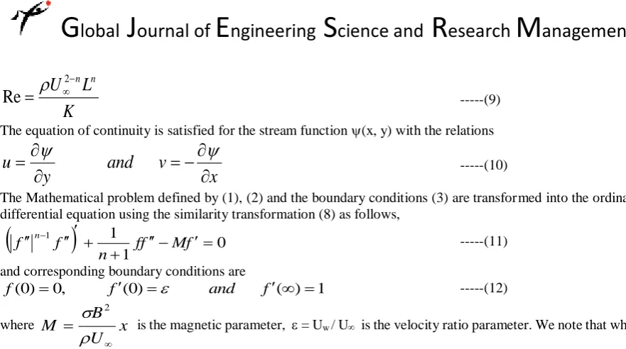
LAMINAR BOUNDARY LAYER FLOW OF A NON-NEWTONIAN POWER LAW
FLUID PAST A MOVING FLAT PLATE
B.Shashidar Reddy*
* Department of Mathematics and Humanities, Mahatma Gandhi Institute of Technology, Gandipet,
Hyderabad-500075, Telangana, INDIA.
KEYWORDS: Magnetic field parameter, Non-Newtonian fluids, power-law index, Quasi-linearization and finite difference method.
ABSTRACT
The steady, two dimensional laminar boundary layer flow of non- Newtonian power-law fluid passing through a continuously moving flat plate under the influence of transverse magnetic field is analyzed. The non-linear partial differential equations governing the flow are transformed into a nonlinear ordinary differential equation using appropriate similarity transformations. This nonlinear ordinary differential equation is linearized by using Quasi-linearization technique and then solved numerically by using implicit finite difference scheme. The system of algebraic equations is solved by using Thomson algorithm. The solution is found to be dependent on various governing parameters including magnetic field parameter M, power-law index n and velocity ratio parameter ε. A systematical study is carried out to illustrate the effects of these major parameters on the velocity profiles. It is found that dual solutions exists when the plate and the fluid move in opposite directions, near the region of separation.
INTRODUCTION
Fluids for which the relationship between the shear stress and rate of strain is nonlinear through the origin at given temperature and pressure are said to be non-Newtonian. The subject of boundary-layer flow on a continuously moving surface traveling through a quiet ambient fluid is currently one of important in view of its relevance to a number of engineering processes. Flows due to a continuously moving surface is encountered in several processes for thermal and moisture treatment of materials, particularly in processes involving continuous pulling of a sheet through a reaction zone, as in metallurgy , in textile and paper industry, in the manufacture of polymeric sheets, sheet glass and crystalline materials. An example for a continuously moving surface is a polymer sheet or filament extruded continuously from die, or a long thread traveling between a feed roll and wind-up roll. Sakiadis [1] was the first to investigate the flow due to sheet issuing with constant speed from a slit into a fluid at rest, he has considered the problem of forced convection along an isothermal moving plate. Tsou et.al [2] studied flow and heat transfer in the boundary layer on a continuously moving surface whereas Soundalgekar and Murthy [3] studied the heat transfer problem by assuming the plate temperature to be variable.
Klemp and Acrivos [4] demonstrated a method for integrating the boundary layer equations through a region of reverse flow and applied it to the problem of uniform flow past a parallel flat plate of finite length whose surface has a constant velocity directed opposite to that of main stream. Similar problems were considered by Abdelhafez [5], Hussaini et. al [6] and Ishak et. al [7]. All of the above investigators, however restrict their analysis to the flow of Newtonian fluids. Most fluids such as molten plastics, artificial fibres, drilling of petroleum, blood and polymer solutions are considered non-Newtonian fluids. Schowalter [8] has introduced the concept of the boundary layer in the theory of non-Newtonian power-law fluids. Acrivos, Shah and Petersen [9] have investigated the steady laminar flow of non- Newtonian fluids over a plate.
Howell et.al [10] and Rao et.al [11] have studied the momentum and heat transfer on a continuous moving surface in a power-law fluid. Kumari and Nath [12] discussed over a continuously moving surface with a parallel free stream.
The object of the present paper is to study the magnetic effects on a steady, two-dimensional laminar flow of a power-law fluid passing through a moving flat plate. The numerical solutions are carried out by using the implicit finite difference scheme.
MATHEMATICAL ANALYSIS
Consider a steady, two dimensional laminar flow of a power-law fluid passing through a moving flat plate with constant velocity Uw, in the same or opposite direction to the free stream U . It is assumed that x – axis extends
parallel to the plate, while the y-axis extends upwards, normal to it. Also, a magnetic field of strength H is applied in the positive y-direction, which produces magnetic effect in the x-direction. The boundary layer equations governing the flow in a power-law fluid can be written as
,
0
y
v
x
u
---(1),
2u
H
y
K
y
u
v
x
u
u
xy
---(2) Subject to the boundary conditionsu = Uw, v = 0 at y = 0,
u U as y ---(3)
where u and v are the velocity components along the x and y axes, respectively, xy is the shear stress and is the
fluid density.
The stress tensor is defined as i.e.
2
2
( 1)2 ij,
n kl kl
xy
K
D
D
D
---(4)where
i j j i ijx
u
x
u
D
2
1
---(5)denotes the stretching tensor, K is the consistency coefficient,
K
is kinematic viscosity and n is thepower-law index. The index n is non-dimensional, and the dimension of K depends on the value of n. The two- parameter rheological eq. (4) is known as the Ostwald-de-waele model or, more commonly, the power-law model. The parameter n is an important index to subdivide fluids into pseudo plastic fluids (n<1) and dilatant fluids (n>1). For n = 1, the fluid is simply the Newtonian fluid. Therefore, the deviation of n from unity indicates the degree of deviation from Newtonian behaviour. With n 1, the constitutive eq. (4) represents shear thinning (n<1) and shear thickening (n>1) fluids. Using eq.s (4) and (5), the shear appearing in eq. (2) can be written as
. 1 y u y u K n xy
---(6)Now the momentum equation (2) becomes
u
H
y
u
y
u
y
y
u
v
x
u
u
n
2 1
---(7)The mathematical problem is simplified by introducing the following dimensionless function f and the similarity variable
.)
(
Re
/
,
/
Re
1 1 1 1
LU
x
L
f
L
y
L
x
n n
---(8)K
L
U
n n
2Re
---(9)The equation of continuity is satisfied for the stream function (x, y) with the relations
x
v
and
y
u
---(10)The Mathematical problem defined by (1), (2) and the boundary conditions (3) are transformed into the ordinary differential equation using the similarity transformation (8) as follows,
01 1 1 f M f f n f
f n ---(11)
and corresponding boundary conditions are
1 ) ( ) 0 ( , 0 ) 0
( f and f
f
---(12)where
x
U
B
M
2is the magnetic parameter, = Uw / U is the velocity ratio parameter. We note that when
= 0 (stationary plate) an n = 1 (Newtonian fluid), the present problem reduces to the classical Blasius problem. When < 0, the fluid and the plate move in the opposite directions, while they move in the same direction when
>0. The case 0 < < 1 is when the speed of the plate is less than those of the fluid and the opposite is true when
>1. Moreover, = 1 corresponds to the case when the plate and the fluid move with the same velocity. For brevity, in this study we consider only the case 1.
NUMERICAL SOLUTION
Since equation (11) is highly non-linear it is difficult to find the closed form solution. Thus first equation (11) is linearized using the Quasi linearization technique [17] to obtain
01 1 ) ( ) ( )
( 1 1 1
f M F F F f f F n F F F f f F
n n n n (13)
where F is assumed to be known.
Now equation (13) with the boundary condition (12) is solved numerically using implicit finite difference scheme and Gauss-Seidel iteration method. The computations were carried out by using C programming. The numerical solutions of are considered as (n+1)th order iterative solutions and F are the nth order iterative solutions. The
step size 0.01 is used to obtain the numerical solution with five decimal place accuracy as the criterion of convergence.
RESULTS AND DISCUSSION
For negative values of there is a critical value c with two solution branches for c<<0, unique solution for
c, a saddle-node bifurcation at = c and no solution for < c. The boundary layer approximation breakdown
at = c and thus no solution is obtained for for < c. These values of c are given in table 1 which are in good
agreement with Klemp and Acrivos [4], Hussaini et .al [6] and Anuar Ishak and Norfifah Bachok [14] for Newtonian fluid. It is seen from the table 1 that the increase of power-law index n decreases the critical value of velocity ratio parameter c.
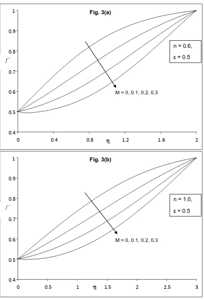
field M is shown in figure 3 with velocity ratio parameter = 0.5 for different fluids such as (a) pseudo-plastic fluid (n = 0.6), (b) Newtonian fluid (n = 1.0) and (c) dilatant fluid (n = 1.4). The effect of magnetic field parameter M is to decelerate the fluid flow velocity f(
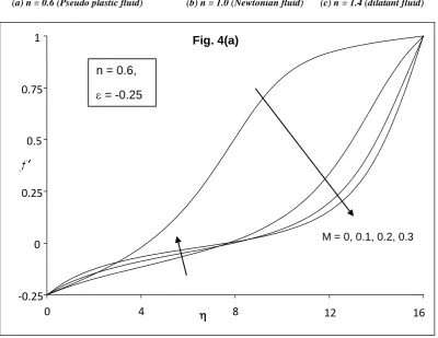
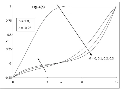
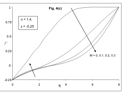
)in all the cases (a), (b) and (c). Figure 4 is shown for velocity profiles f(
) (upper branch) for different values of magnetic field parameter M with velocity ratio parameter - -0.25 for different fluids such as (a) pseudo-plastic fluid (n = 0.6), (b) Newtonian fluid (n = 1.0) and (c) dilatant fluid (n = 1.4). The effect of magnetic field parameter M is to reduce the velocity profiles f(
)far away from the plate and reverse phenomenon is observed near the plate.NOMENCLATURE
B – Magnetic field intensity Dij – stretching tensor
f - Dimensionless stream function K – consistency coefficient
L – Characteristic length of the plate n – power-law index
Re – generalized Reynolds number Uw – Free stream velocity
u, v – Velocity components along and normal to the plate x, y - Coordinates along and perpendicular to the plate η – Dimensionless similarity variable
- stream function ρ – Densityσ – Electrical conductivity ε – velocity ratio parameter τxy - Shear stress
REFERENCES
1. Sakiadis BC. Boundary layer behaviour on continuous moving solid surfaces. AIChE J. 1961; 7: 26-28. 2. Tsou FK, Sparrow EM, Goldstein RJ. Flow and heat transfer in the boundary layer on a continuous
moving surface. Int J Heat Mass Transfer. 1967; 10: 219-235.
3. Soundalgekar VM, Murty TV. Heat transfer in flow past a continuous moving plate with variable temperature. Wärme-und stöffübertrag-ung. 1980; 14: 91-93.
4. Klemp JB, Acrovos A. A method for integrating the boundary-layer equations through a region of reverse flow. J. Fluid Mech. 1972; 53: 177-191.
5. Abdelhafez TA. Skin friction and heat transfer on a continuous flat surface moving in a parallel free stream. Int. J. Heat Mass Transfer. 1985; 28: 1234-1237.
6. Hussaini MY, Lakin WD. A. Nachman, On similarity solutions of a boundary layer problem with an upstream moving wall. SIAM J. Appl. Math. 1987; 47: 699-709.
7. Ishak A, Nazar R, Arifin NM, Pop I. Dual solutions in magnetohydrodynamic mixed convection flow near a stagnation-point on a vertical surface. ASME J. Heat Transfer. 2007; 129: 1212-1216.
8. Schowalter WR. The application of boundary-layer theory to power-law theory to power-law pseudo-plastic fluid : Similarity solutions. AIChE J. 1960; 6: 24-28.
9. Acrovos A, Shah MJ, Petersen EE. Momentum and heat transfer in laminar boundary-layer flows of non-Newtonian fluids past external surfaces. AIChE J. 1960; 6: 312-317.
10. Howell TG, Jeng DR, De Witt KJ. Momentum and heat transfer on a continuous moving surface in a power law fluid. Int. J. Heat and Mass Transfer. 1997; 40: 1853-1861.
11. Rao JH, Jeng DR, De Witt KJ. Momentum and heat transfer in a power-law fluid with arbitrary injection/suction at a moving wall. Int. J. Heat Mass Transfer. 1999; 42: 2837-2847.
12. Kumari M, Nath G. MHD boundary-layer flow of a non-Newtonian fluid over a continuously moving surface with a parallel free stream. Acta Mechanica.2001; 146: 139-150.
13. Mahmoud MAA, Mahmoud MAE. Analytical solutions of hydromagnetic boundary-layer flow of a non-Newtonian power-law fluid past a continuously moving surface. Acta Mechanica. 2006; 181: 83-89. 14. Saritha K, Rajasekhar MN, Shashidar Reddy B. Quasi-Linearization approach to Effects of Heat
plate with heat flux and Viscous dissipation. International journal of applied science and engineering research. 2015; 4(1) : 36-56.
15. Kishan N, Shashidar Reddy B. Viscous Dissipation effects on mhd flow of a conducting power-law fluid with a pressure gradient. International Journal of applied mechanics and engineering. 2012; 17: 101-112. 16. Anuar Ishak, Norfifah Bachok. Power-law fluid flow on a moving wall. European J of Scientific
Research. 2009; 34: 55-60
17. Bellman RE, Kalaba RE. Quasi-Linearization and Non-linear boundary value problem. Elsevier: NewYork; 1965.
Table 1: Variation of c power-law index n
n c
0.6 -0.3532
0.8 -0.3641
1.0 -0.3816
1.2 -0.3975
1.4 -0.4996
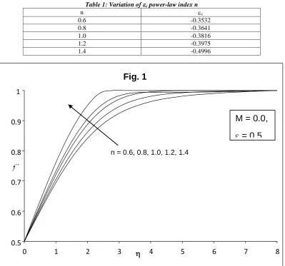
Fig. 1. Velocity Profiles ffor different values of power-law index n with = 0.5 and M = 0.0.
0.5 0.6 0.7 0.8 0.9 1
0 1 2 3 4 5 6 7 8
n = 0.6, 0.8, 1.0, 1.2, 1.4
M = 0.0,
= 0.5
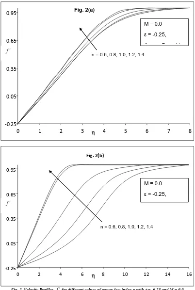
Fig. 2. Velocity Profiles ffor different values of power-law index n with = -0.25 and M = 0.0. (a) Lower Branch (b) Upper Branch
-0.25
0.05
0.35
0.65
0.95
0
1
2
3
4
5
6
7
8
Fig. 2(a)
M = 0.0
= -0.25,
(Lower Branch)
n = 0.6, 0.8, 1.0, 1.2, 1.4
-0.25 0.05 0.35 0.65 0.95
0 2 4 6 8 10 12 14 16
Fig. 2(b)
M = 0.0
= -0.25,
(Upper Branch)
0.4 0.5 0.6 0.7 0.8 0.9 1
0 0.4 0.8 1.2 1.6 2
M = 0, 0.1, 0.2, 0.3
n = 0.6,
= 0.5
Fig. 3(a)
0.4 0.5 0.6 0.7 0.8 0.9 1
0 0.5 1 1.5 2 2.5 3
M = 0, 0.1, 0.2, 0.3
n = 1.0,
= 0.5
Fig. 3. Velocity Profiles f for different values of Magnetic parameter M with = 0.5. (a) n = 0.6 (Pseudo plastic fluid) (b) n = 1.0 (Newtonian fluid) (c) n = 1.4 (dilatant fluid)
0.4 0.5 0.6 0.7 0.8 0.9 1
0 0.5 1 1.5 2 2.5 3
Fig. 3(c)
M = 0, 0.1, 0.2, 0.3
n = 1.4,
= 0.5
-0.25 0 0.25
0.5 0.75 1
0 4 8 12 16
M = 0, 0.1, 0.2, 0.3 n = 0.6,
= -0.25
-0.25 0 0.25
0.5 0.75 1
0 4 8 12
n = 1.0,
= -0.25
Fig. 4(b)
Fig. 4. Velocity Profiles f for different values of Magnetic parameter M with = -0.25. (a) n = 0.6 (Pseudo plastic fluid) (b) n = 1.0 (Newtonian fluid) (c) n = 1.4 (dilatant fluid)
-0.25 0 0.25
0.5 0.75 1
0 2 4 6 8
n = 1.4,
= -0.25
Fig. 4(c)