Vol. 11, No. 4, 2019 Article ID IJIM-1222, 9 pages Research Article
A New Two-stage Iterative Method for Linear Systems and its
Application in Solving the Poisson’s Equation
F. Shariffar ∗, A. H. Refahi Sheikhani †‡
Received Date: 2018-08-28 Revised Date: 2019-03-11 Accepted Date: 2019-03-13
————————————————————————————————–
Abstract
In the current study, we investigate the two-stage iterative method for solving linear systems. In this regard, a new comparison theorem for the spectral radius of two-stage iterative method with different inner and outer splitting matrices under suitable conditions is presented. Our new theorem shows which splitting generates fast convergence in iterative methods. Finally, based on the Poisson’s equation, we solve the Poisson-Block tridiagonal matrix by two different splittings, which is an issue that is frequently encountered in mechanical engineering and theoretical physics. Based on a particular linear system, numerical computations are presented, which clearly show the reliability and efficiency of the presented algorithm.
Keywords: Two stage iterative method; Splitting; Comparison theorem; Spectral radius.
—————————————————————————————————–
1
Introduction
C
otionsnsider the following system of linearequa-Ax=b, (1.1)
where A ∈ Rn×n and b, x ∈ Rn. Linear sys-tems1.1 occur in a wide variety of areas, includ-ing numerical differential equations, eigenvalue problems, economics models, design and com-puter analysis of circuits, power system networks, chemical engineering processes, physical and bio-logical sciences. See [16,17,21,26,30,31,14], for discussion of such applications. For any splitting,
∗Department of Mathematics, Lahijan Branch, Islamic Azad University, Lahijan, Iran.
†Corresponding author. ah [email protected], Tel: +98(911)3475547.
‡Department of Mathematics, Lahijan Branch, Islamic Azad University, Lahijan, Iran.
A=M −N withdet(M) ̸= 0 the basic iterative methods for solving1.1 is
xi=M−1N xi−1+M−1b, i= 1,2, ... (1.2)
The spectral radius of a real square matrix A
is the maximum moduli of the eigenvalues of
A, which is denoted by ρ(A). For a splitting
A = M −N the iteration scheme 1.2 converges to the unique solution x = A−1b for any ini-tial vector value, if and only if ρ(M−1N) < 1 , where T = M−1N is called the iteration ma-trix. There are some popular iterative meth-ods for solving linear systems 1.1 based on 1.2; for instance, Jacobi, Gauss-Seidel, SOR, etc. [13, 15, 19, 20, 22, 25, 28, 29, 32]. The meth-ods of the above-mentioned models, proceed by solving at each step a simpler system; however, when this system is itself solved by an inner iter-ative method, the global method is called a two-stage iterative method. This method is one of
the drastic choices for getting the numerical so-lutions of linear systems. The two-stage itera-tive method was first proposed by Nichols [12] in 1973 for solving systems of linear equations; but then has been extensively studied by many au-thors [3,5, 6,7, 11,18,23,24,1]. This method, also called the inner/outer method, consists of ap-proximating the linear system1.2 by using inner iterations; i.e., let A = M −N and the split-ting M =F −Gperform, say (s(k)) inner itera-tions. In this regard, some comparison theorems for splittingA=F1−G1−N =F2−G2−N have
been proposed in the literature [2,4,8,9,27]. In this paper, On the basis of nonnegative matrix theory, we present a new comparison theorem for the convergent splittings of two iteration matri-ces, induced by our proposed method. But up to now, no study has discussed comparison the-orems when both inner and outer iterations are different splittings (i.e N1 ̸=N2). So, this paper
is planning to fill in this gap and reach a com-parison theorem for two-stage iterative methods under different conditions. Our new comparison theorem shows that which splitting produces less error, which is considered the better one then. This paper is organized as follows. After review-ing the two-stage iterative method and introduc-ing some related essential concepts and results in Section 2, we further set up our new results in Section 3. The convergence analysis and error bounds of our method will be presented in this Section. In Section4, we examine the advantages of our results by carrying out numerical computa-tions. For example, we solved the Poisson-Block tridiagonal matrix from the Poisson’s equation perspective, which arises in mechanical engineer-ing and theoretical physics. Finally, conclusions are presented in Section5.
2
Preliminaries
Consider the linear system 1.1 with outer split-tingA=M−N and inner splitting M =F−G. Then the algorithm of two-stage iterative method is as follows. Algorithm1.
Step 1.
Choose an initial vector x0, tol, number of outer
iteration m and sequence of number of inner it-erations, s(k), k= 1, ..., m.
Step 2.
For i= 1, ..., mdo
y0 =xi−1
For j= 1, ..., s(k)
F yj =Gyj−1+N yi−1+b
xi=ys(k).
Step 3.
Ifb−Axi ≤tol, then stop; otherwise, seti=i+ 1
and go to Step 2.
When the number of inner iterations is fixed in each outer step, i.e.,s(k) =s,s≥1, it is said that the method is stationary, while a non-stationary two-stage method is such that the number of in-ner iterations may change with the outer itera-tions. Throughout the current paper, it is as-sumed that s(k) =s,s≥1.
By replacing the loop overj and by1.2, the two-stage iterative methods for solving the system of linear equations 1.1have the following form
xi = (F−1G)sxi−1+
+∑sj−=01(F−1G)jF−1(N xi−1+b),
i= 1,2, ...
(2.3)
Clearly, the iteration matrix corresponding to2.3
is
Ts= (F−1G)s+ ∑s−1
j=0(F−1G)jF−1N
=I−(I−(F−1G)s)(I−M−1N) (2.4)
where I denotes the n×nidentity matrix. Ifρ(F−1G)<1, thenI−(F−1G)sis nonsingular. Then there exists a unique pair of matrices [10],
Bs and Cs, such that M = Bs−Cs and R =
(F−1G)s=Bs−1Cs where
Bs=M(I−R)−1, (2.5)
Cs =M(I−R)−1R, (2.6)
Ts=B−s1(Cs+N). (2.7)
3
Main results
In this section we present a new theorem under suitable conditions. Based on this theorem, we can find which double splitting is more efficient compared with other ones. We should begin with some basic notations and preliminary results first.
Definition 3.1 Let A be a real matrix. The splitting A=M−N is called
(a) convergent if ρ(M−1N)<1,
(b) regular if M−1 ≥0 and N ≥0, and
(c) weak regular if M−1 ≥0 and M−1N ≥0.
Lemma 3.1 Let A = M −N be a convergent regular splitting, and let R ≥ 0, ρ(R) < 1. If the unique splitting is as M =Bs−Cs such that
R =Bs−1Cs is a weak regular splitting, then the
two-stage iterative method for any nonnegative s
of inner iterations will be convergent.
Proof. see [10].
Lemma 3.2 Let A = M −N be regular or a weak regular splitting of A. Thenρ(M−1N) <1 if and only if A−1 ≥0.
Proof. see [2].
Lemma 3.3 Let A = M1 −N1 = M2 −N2 be
two weak regular splitting of A, where A−1 ≥0. If M1−1≥M2−1, then ρ(M1−1N1)≤ρ(M2−1N2).
Proof. see [12].
Now, we establish new results in the following theorem.
Theorem 3.1 Let A−1 ≥ 0, A = M1 −N1 =
M2−N2 be regular splitting and letM1 =F1−G1,
M2 =F2−G2 be weak regular splitting. IfM2−1 ≥
αM1−1 then
ρ(Ts(M2−N2))≤ρ(Ts(M1−N1))<1
where α= 1−ρ1
1−ρ2 with ρi =ρ(F
−1
i Gi) for i= 1,2.
Proof. By Lemma 3.1, it is easy to show that ρ(Ts(M1−N1)) < 1. But by two-stage
it-erative method (Algorithm1), fori= 1,2 we have
A=Mi−Ni,
Mi=Fi−Gi =Bi,s−Ci,s
and
Ri = (Fi−1Gi)s=B−i,s1Ci,s,
so we get that
A=Mi,T −Ni,T,
where
Mi,T =Bi,s=Mi(I−Ri)−1
and
Ni,T = (Ci,s+Ni) =Mi(I−Ri)−1Ri+Ni.
Since A = Mi−Ni are regular splittings, Mi =
Fi−Gi is the weak regular splitting. By Lemma 3.2, ρ1, ρ2 < 1. Furthermore, it can be shown
that A = M(i, T)−N(i, T) is the weak regular
splitting. Therefore, to apply Lemma 3.3, it is only necessary to show that M2−,T1 ≥M1−,T1. Since
M2−1≥αM1−1, we have
(1−ρ(F2−1G2))M1 ≥M2(1−ρ(F1−1G1)).
Since
GF−1=F(F−1G)F−1,
we have
ρ(GF−1) =ρ(F−1G),
so
(I−(G2F2−1))M1≥M2(I−(F1−1G1))
⇒(I−(G2F2−1)s)M1 ≥M2(I−(F1−1G1)s)
⇒M2−1(I−(G2F2−1)s)≥(I−(F1−1G1)s)M1−1
⇒M2−1−M2−1(G2F2−1)s≥(I −R1)M1−1.
Since
M(F−1G)s= (GF−1)sM,
we have
(I−(F2−1G2)s)M2−1 ≥(I−R1)M1−1,
4
Examples
In this section, as an application of Theorem3.1, we give some examples to illustrate the results that have been obtained in the previous sections. We use the number of inner iteration ass(k) =s,
s≥1. Moreover, we denote the number of outer iteration bym.
Example 4.1 Let A=
(
1 −1
−1.5 1.9
)
where
M1=
(
1.1 −0.9
−0.9 2.1 )
, F1=
(
2.1 −1.8
−1.6 5.1 )
,
G1=
(
1 −0.9
−0.7 3 )
, N1=
(
0.1 0.1 0.6 0.2
) .
M2=
(
1 −1
−1 2 )
, F2=
(
1.25 −1.8
−1.25 3.6 )
,
G2=
(
0.25 −0.8
−0.25 1.6 )
, N2=
(
0 0
0.5 0.1 )
.
It is not difficult to examine splittings as defined in Theorem3.1 Furthermore
α = 0.6609
αM1−1=
(
0.9253 0.3965 0.3965 0.4847
) < ( 2 1 1 1 )
=M2−1.
Hence, Theorem3.1implies the following inequal-ity
ρ(Ts(M2−N2))≤ρ(Ts(M1−N1))≤1,
∀s≥1.
(4.8)
In fact, by computations, Table. 1shows that our theorem holds for the above matrix.
In this exampleA−1 =
(
4.75 2.5 3.75 2.5
)
, so the
ex-act solution of the systemAx=bwithb= (1,2)T is (394,3547)T. We report the numerical solution er-rors of this system in Table. 2 with initial vector valuev0 = (8,8)T. From Table. 2we can see that
errors generated by second splitting are less than errors generated by first splitting with the same inner and outer iterations.
Remark 4.1 Moreover if the matrix is large then we can use the Krylov subspace methods.
With this method we can theN-dimensional prob-lem onto nested Krylov subspaces of increasing di-mension. We now consider methods for improv-ing the accuracy. Let x be approximated solution with Krylov subspaces method to the linear sys-tem of equations Ax = b and let r = b−Ax
be the corresponding residual vector. Then one can attempt to improve the solution by solving the system Aδ =r for a correction δ and taking
xc=x+δ as a new approximation. If no further
rounding errors are performed in the computation of δ this is the exact solution. Otherwise this re-finement process can be iterated.
Example 4.2 In this example we consider linear
system Ax=b with
10 −11 −01
−1 0 2
and b=
(−1,2,0.5)T.
The exact solution of this system is (2.5,3.5,1)T. It is easy to see that A−1 ≥ 0. Some regular splitting ofA=M−N and weak regular splitting of M =F −Gare given below.
M1=
10 −11 −11
−1 0 2 , F1=
10 −11 −11
−1 0 2 ,
G1=
00 00 00 0 0 0
, N1=
00 00 10 0 0 0
.
M2=
10 01 −01 0 0 2
, F2=
10 01 −01 0 0 3
,
G2=
00 00 00 0 0 1
, N2=
00 10 00 1 0 0
.
M3=
10 −11 −01
0 0 2
, F3=
10 01 −01 0 0 3
,
G3=
00 10 00 0 0 1
, N3=
00 00 00 1 0 0
.
In this example we denote 1−ρi
1−ρj withαi,j. For
the above splitting of A we have
Table 1: Spectral radii of iteration matrices in example4.1.
s ρ(Ts(M1−N1)) T˙s(M˙2-N˙2)
1 0.9002 0.7072
2 0.8392 0.6295
3 0.8019 0.6092
4 0.7791 0.6033
5 0.7652 0.6013
Table 2: Numerical solution errors in example4.1.
s m by first splitting by second splitting
10 20 0.0381 5.5871×10⁻⁴
20 30 7.7560×10⁻⁴ 4.7439×10⁻⁷
30 40 6.6980×10⁻⁵ 2.0870×10⁻⁹
40 50 3.6971×10⁻⁶ 1.2394×10⁻¹¹
50 60 1.9139×10⁻⁷ 6.9095×10⁻¹⁴
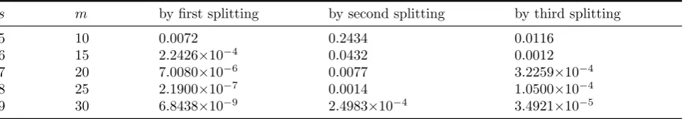
Table 3: Numerical solution errors in example4.2.
s m by first splitting by second splitting by third splitting
5 10 0.0072 0.2434 0.0116
6 15 2.2426×10⁻⁴ 0.0432 0.0012
7 20 7.0080×10⁻⁶ 0.0077 3.2259×10⁻⁴
8 25 2.1900×10⁻⁷ 0.0014 1.0500×10⁻⁴
9 30 6.8438×10⁻⁹ 2.4983×10⁻⁴ 3.4921×10⁻⁵
Table 4: Results of example4.3with s=50.
n noGJ error ofGJ noJ G error ofJ G
4 55 6.8978×10⁻¹⁰ 103 2.0283×10⁻⁹
8 171 2.0555×10⁻⁸ 327 4.6248×10⁻⁸
16 575 5.6102×10⁻⁷ 1106 1.1536×10⁻⁶
and
M1−1 =
01.5 11.5 00.5 0.5 0.5 0.5
≥
0.66670 0.66670 0.33330
0 0 0.3333
=α2,1M2−1,
M3−1=
10 11 00..55 0 0 0.5
≥
10 01 00.5 0 0 0.5
=α2,3M2−1.
Hence, Theorem3.1implies the following inequal-ities for all s
ρ(Ts(M1−N1))≤ρ(Ts(M2−N2))≤1, (4.9)
ρ(Ts(M3−N3))≤ρ(Ts(M2−N2))≤1. (4.10)
For initial vector value (0,0,0)T the errors gen-erated by above spilittings are shown in Table. 3
with the same inner and outer iterations.
Figs. 1,2, and Table. 3we can find that the first splitting converges to the exact solution faster than the third splitting, and the same happens for the third splitting compared with the second splitting. This is supported by inequalities 4.9
and 4.10.
Example 4.3 Poisson Block tridiagonal matrix from Poisson’s equation.
The Poisson equation is a very powerful tool for modeling the behavior of electrostatic systems, al-though it might be only solved analytically for very simplified models. Consequently, a numer-ical simulation must be utilized in order to model the behavior of complex geometries with practi-cal values. In two-dimension spaces, the Poisson equation can be written as
∂2u ∂x2 +
∂2u ∂y2 =ρ,
where uis the unknown function andρ is a given function.
The finite difference method is based on local ap-proximations of the partial derivatives in a Par-tial DifferenPar-tial Equation, which are derived by low order Taylor series expansions. The method is quite simple to define and rather easy to im-plement. Also, it is particularly appealing for simple regions, such as rectangles, and when uni-form meshes are used. The matrices that result from these discretizations are often well struc-tured, which means that they typically consist of a few nonzero diagonals. Today, Finite-difference methods are the dominant approach to numerical solutions of partial differential equations. Using the finite difference numerical method, the dis-cretization of the two dimensional Poisson equa-tion can be written as
Ax=b, (4.11)
where matrix A is a block tridiagonal matrix of ordern2, and it called the poisson matrix. To
pro-duce a poisson matrix of dimension n, one may use the MATLAB command
A=gallery(′poisson′, n).
For solving system 4.11 through using the two-stage iterative method with initial vector zeroes,
we consider the classical iterative methods such as Jacobi and Gauss-Seidel for inner and outer iteration.
First splitting.
In this case, we apply Gauss-Seidel’s method to outer iteration and Jacobi’s method for inner it-eration, i.e., A=MG−NG,MG =FJ −GJ.
Second splitting.
We use Jacobi and Gauss-Seidel method to outer and inner iterations, respectively, i.e. A=MJ−
NJ,MJ =FG−GG.
It is not difficult to examine that splittings are defined as in Theorem 3.1. Furthermore:
α= 1,
and
MG−1 ≥MJ−1,
hence Theorem 3.1implies that the first splitting performs much better than second splitting. The results of the numerical solution of system 4.11
with (1,1,1, ...,1)T are shown in Table4, where in Table4,noGJ and noJ G denote number of outer
splitting of first and second splitting respectively. The stopping criterion for outer iteration m is
∥xi−xi−1∥2
∥xi∥2 <10
−10, wherex
i is the numerical
so-lution in the i’th iteration.
In Table4, we report the number of iterations for the corresponding splitting of A with different n
for s = 50 (number of inner iterations) and the numerical errors as ∥exact−numerical∥2.
The results of Table4were supported by theorem
3.1, and the first splitting performs much better than the second splitting.
5
Conclusions
In this paper, we have studied the two-stage iter-ation method for solving systems of linear equa-tions. Moreover, we have discussed comparison theorems when both inner and outer iterations are different splittings (i.eN1 ̸=N2). By this
100 101 102
log m 10-15
10-10
10-5
100
105
logarithm of generated errors
s=10
first splitting second splitting third splitting
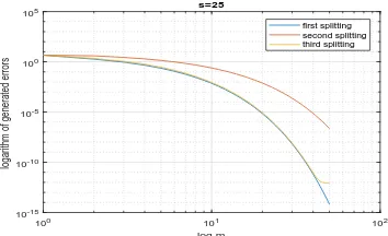
Figure 1: Comparison of error of spltttings with inner iteration s = 10 and outer iteration m = 1,2,3, ...,50 in Example 4.2.
100 101 102
log m 10-15
10-10
10-5
100
105
logarithm of generated errors
s=25
first splitting second splitting third splitting
Figure 2: Comparison of error of spltttings with inner iteration s = 25 and outer iteration m = 1,2,3, ...,50 in example4.2.
In Example 4.2 we consider three different split-tings. The results in Table. 3, Figs. 1, and
2 show that which splitting converges fast and works with high accuracy. This result was sup-ported by our new theorem. Moreover, in Exam-ple 4.3 we solved the Poisson-Block tridiagonal matrix from Poisson’s equation by two different splittings, which arises in mechanical engineering and theoretical physics. In this regard, Table 4
shows that it is important to choose the appro-priate splitting.
References
[1] H. Aminikhah, A. H. Refahi Sheikhani, H. Rezazadeh, Exact solutions for the frac-tional differential equations by using the first integral method, Nonlinear Engineering 4 (2015) 15-22.
[2] Z. Z. Bai, The convergence of the two-stage iterative method for Hermitian positive def-inite linear systems, Appl. Math. Lett. 11 (1998) 1-5.
[3] Z. Z. Bai, M. Rozloznik, On the numerical behavior of matrix splitting iteration meth-ods for solving linear systems,SIAM Journal on Numerical Analysis 53 (2015) 1716-1737.
[4] Z. H. Cao, Convergence of nested iterative methods for symmetric P-regular splittings, SIAM J. Matrix. Anal. Appl. 22 (2000) 20-32.
[5] J. J. Climent, C. Perea, Some comparison theorems for weak nonnegative splittings of bounded operators,Linear Algebra Appl.275 (1998) 77-106.
[6] R. Couturier, L. Z. Khodja, A scalable mul-tisplitting algorithm to solve large sparse lin-ear systems, The journal of Supercomputing 71 (2015) 1345-1356.
[7] M. Dehghan, M. Hajarian, Asynchronous Multisplitting GAOR Method and Asyn-chronous Multisplitting SSOR Method for Systems of Weakly Nonlinear Equations, Mediterranean Journal of Mathematics 7 (2010) 209-223.
[8] A. Frommer, D. B . Szyld, Asynchronous two-stage iterative methods, Numer. Math. 69 (1994) 141-153.
[9] R. Garrappa, An analysis of convergence for two-stage wave form relaxation methods, J. Compute. And Appl. Math. 169 (2004) 377-392.
[10] P. J. Lanzkron, D. J. Rose, D. B. Szyld, Con-vergence of nested iterative methods for lin-ear systems, Numer. Math. 58 (1991) 685-702.
[11] M. Mashoof, A. H. Refahi Sheikhani, Sim-ulating the solution of the distributed or-der fractional differential equations by block-pulse wavelets, UPB Scientific Bulletin, Se-ries A: Applied Mathematics and Physics 79 (2017) 193-206.
[13] N. K. Nichols, On the convergence of two-stage iterative processes for solving lin-ear equations, SIAM Journal on Numerical Analysis 10 (1973) 460-469.
[14] A. H. Refahi Sheikhani, A. Ansari, H. Saberi Najafi, F. Merhdoust, Analytic study on lin-ear systems of distributed order fractional differential equations, Le Matematiche 67 (2012) 3-13.
[15] H. Rezazadeh, H. Aminikhah, A. H. Re-fahi Sheikhani, Stability analysis of Hilfer fractional differential systems,Mathematical Communications 21 (2016) 45-64.
[16] H. Saberi Najafi, S. A. Edalatpanah, A New family of (I+S)-type preconditioner with some applications, computational and ap-plied mathematics 34 (2015) 917-931.
[17] H. Saberi Najafi, S. A. Edalatpanah, On the iterative methods for weighted linear least squares problem,Engineering Computations 33 (2016) 622-639.
[18] H. Saberi Najafi, S. A. Edalatpanah, A. H. Refahi Sheikhani, Convergence Analysis of Modified Iterative Methods to Solve Linear Systems, Mediterranean Journal of Mathe-matics 11 (2014) 1019-1032.
[19] H. Saberi Najafi, A. H. Refahi Sheikhani, FOM-inverse vector iteration method for computing a few smallest (largest) eigenval-ues of pair (A, B),Applied mathematics and computations 188 (2007) 641-647.
[20] H. Saberi Najafi, A. H. Refahi Sheikhani, M. Akbari, Weighted FOM-inverse vector itera-tion method for computing a few smallest (largest) eigenvalues of pair (A, B), Applied mathematics and computation 192 (2007) 239-246.
[21] H. Saberi Najafi, A. H. Refahi Sheikhani, M. Akbari, A new restarting method in the Lanczos algorithm for generalized eigenvalue problem,Applied mathematics and computa-tion 184 (2007) 421-428.
[22] H. Saberi Najafi, S. A. Edalatpanah, A.H. Refahi Sheikhani, An analytical method as a
preconditioning modeling for systems of lin-ear equations, Comp. Appl. Math.37 (2016) 922-931.
[23] R. S. Varga, Matrix Iterative Analysis, sec-ond ed., Springer, Berlin (2000).
[24] R. S. Varga, Matrix Iterative Analysis, En-glewood Cliffs:Prentice-Hall (1981).
[25] G. Wang and N. Zhang, New preconditioned AOR iterative method for Z-matrices, J. Appl. Math. Comput.37 (2011) 103-117.
[26] L. Wang, Semiconvergence of two-stage it-erative methods for singular linear sys-tems,Linear Algebra and its applications422 (2007) 824-838.
[27] C. L. Wang, G. Y. Meng, Parallel multisplit-ting two-stage iterative methods with gen-eral weighting matrices for non-symmetric positive definite systems,Applied Mathemat-ics Letters 26 (2013) 1065-1069.
[28] S. L. Wu, T. Z. Huang, C. X. Li, Modi-fied block preconditioners for the discretized time-harmonic Maxwell equations in mixed form, J. Computational Applied Mathemat-ics 237 (2013) 419-431.
[29] X. Yang, Y. Huang, An estimation of outer iteration number in inexact splitting itera-tion methods,J. Communication on Applied Mathematics and Computation 31 (2017) 191-199.
[30] D. M. Young, Iterative solution of large linear systems, Academic Press, New York (1971).
[31] J. H. Yun, S. W. Kim, Convergence of two-stage iterative methods using incomplete factorization, J.Comput. Appl. Math. 166 (2004) 565-580.
Farhad Shariffar has got his B.Sc. degree in applied Mathematics from University of Guilan and his M.Sc. degree from Islamic Azad University of Lahijan Branch. He received his Ph.D. degree in the field of Applied Mathematics in 2018. He is currently an Assistant Professor at Islamic Azad University, Fuman Branch. His re-search interests are in the areas of applied math-ematics including Numerical Linear Algebra.