Preliminary GIS elaborations
to apply rapid flood spreading models
Giulia Farina
1*†, Anna Bernini
1, Stefano Alvisi
1and Marco Franchini
1 1 Engineering Department, University of Ferrara, Ferrara, Italy[email protected], [email protected], [email protected], [email protected]
Abstract
Flood risk analysis involves simulating many scenarios from which to draw statistical information about flood extent and depth. Rapid but still sufficiently accurate models enabling flooded areas to be delimited using a DEM have been introduced in the scientific literature. These models, called Rapid Flood Spreading Models (RFSMs), are based on highly simplifying hydraulic assumptions while make large use of GIS information and elaborations. Three different RFSMs are here applied to a test case, largely characterized by flat land. The results obtained are compared with those of a two-dimensional hydraulic model confirming the possibility of preliminarily elaborating topographic GIS data to easily gain geometric information on flooded areas through geospatial analysis.
1
Introduction
Flooding is a dramatic problem worldwide. Against the backdrop of climate and land-use changes, demographic growth and urban development in flood-prone areas, the causes of floods are shifting and their tremendous impacts on society, economy and environment are accelerating (1).
For the definition of flood risk management plans (2), the challenge is to understand the flood dynamics in order to assess and manage its repercussions. For this purpose, two-dimensional hydraulic models are widely used to represent a flood event, the best known commercially available are MIKE21 (3), SOBEK (4) and TELEMAC-2D (5). The hydraulic models are capable to simulate the flood phenomenon starting from its trigger point or points, providing sufficient information related to timing, extent, speed and water depth. When all these main flood characteristics are known, it is possible to develop relevant management strategies and set up suitable regulation in order to safeguard the affected areas. In this context, it is therefore often necessary to perform several simulations, for example by varying some input parameters of the model to make it closer to reality,
* Masterminded EasyChair and created the first stable version of this document † Created the first draft of this document
Volume 3, 2018, Pages 684–691
or simulating different scenarios to design the most appropriate mitigation actions. Thus, the computational speed plays a fundamental role. In order to make the simulating process faster, numerous studies have aimed to define simplified approaches based on diffusive formulations (6), or on pairing a 1D model (used to study propagation in the riverbed) with a 2D model (used to represent the submersion wave), or based on cellular automata, which by their very nature enable implementation of the parallel type of computing code (7).
Though all of the aforesaid simplified models can achieve good levels of computational efficiency, they are not sufficiently fast because they take into consideration the complete temporal evolution of the hydraulic process. Their computational demands become prohibitive especially in flood risk analysis and recourse must be made to faster methods, in particular the Rapid Flood Spreading Models (RFSMs). The peculiarity of these models consists in entirely disregarding the temporal evolution of the flood phenomenon ( (8), (9), (10)). Due to their intrinsic nature, these models provide the flood depth associated to the maximum flooded area when the flood has reached its final state, i.e. water is still everywhere, while timing and velocity fields are not considered.
All the RFSMs consist of two phases: in the first pre-processing phase, an array of storage reservoirs is constructed from a digital elevation model (DEM) of the potentially flooded area. In the second spreading phase, a specified volume of flood water is assigned to an initial accumulation zone (or storage reservoir) and distributed on and across the adjacent accumulation zones.
The pre-processing routine implementation can be developed within the framework of a Geographic Information System (GIS) for instance using the ArcGISTM / ArcHydro software (11) which supplies a suite of terrain pre-processing tools that aid in the manipulation of DEM (12).
In addition to the pre-analysis for the construction of flood maps, ArcHydro software has found application in several studies as starting point for water resource analyses: it allows to create base-maps and GIS data that support later simulations using hydrologic (soil type, land-use, vegetation) and topographic (area, slope) information (13), incorporate man-made structures into stream networks to develop an integrated data and flow modelling environment for asset management and hydrologic modelling support (14), develop data inputs for external hydrologic and hydraulic models (15), display simulation results on a map and integrate them with other GIS analyses.
This study focuses on the detailed description of the preliminary pre-processing operations performed in ArcHydro environment, fundamental for the RFSMs application to real case studies. The paper is organized as follow. Initially, in Section 2, with reference to the Argenta case study (Italy) the overall ArcGISTM / ArcHydro framework is outlined: in particular, the construction procedures of both the accumulation zones and boundary lines are described in detail. Section 3 gives a brief reminder of the RFSMs while for deeper information the reader can refer to (8), (9), (10)). Then Section 3 presents the subsequent application of these rapid models to a potential flood event in Argenta zone, highlighting how the information directly derived from GIS become indispensable input for the RFSMs. Finally, the resulting flooded areas and depths are compared with those computed by the 2D hydraulic model FLO-2DTM (16), the latter considered to be the correct results and used to measure the RFSMs accuracy. Conclusions are provided in Section 4.
2
The terrain pre-processing phase
2.1
The case study
Figure 1: Digital elevation model (DEM) of the Argenta study area.
This area is substantially flat, with elevations that range between -3.37 and 14.74 m a.s.l. but the main percentage of area (about 80 %) is characterized by elevation less than 3 m and the average elevation is equal to 0.81 m a.s.l.. As can be seen in Figure 1, it is worth noting that DEM cells with elevation more than 10 m are mainly due to river banks or streets.
2.2
The pre-processing ArcGIS
TM/ ArcHydro framework
The pre-processing phase is aimed to build up a system of storage reservoirs (or accumulation zones AZs) starting from the digital elevation model (DEM) of the investigated flooded area and deduces its main geometrical characteristics.
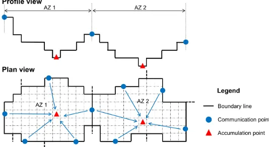
Figure 2 shows the sketch of the subdivision of a generic DEM into a system of AZs. The single AZ represents the natural depression in the ground where water flows toward in case of flooding and has several contiguous cells.
Figure 2: Sketch of the subdivision of the DEM into a system of accumulation zones (AZs) with the associated boundary lines, communication points and accumulation points.
which water spills into a neighbour AZ. Basically, there is one communication point for each line of separation and one line of separation for each AZ adjacent to the one considered.
The pre-processing phase is essential for the execution of the subsequent spreading phase because it defines a system of AZs that is unique and represents the calculation domain of the spreading phase where water can move and then accumulate. Thus, depending only on the terrain topography, the preliminary operations need to be performed only once. In this study they were accomplished in ArcGISTM environment using a suite of ArcHydro tools particularly dedicated to both the manipulation of DEM and the necessary geometrical information extraction. Operatively, the pre-processing phase features several steps, to be performed one after the other, as detailed in Table 1. In the following a detailed description of each of these steps, together with indication of the ArcHydro tool used to perform them, is provided.
1 2 3 4 5 6
ArcHydr o Tool Sink Prescreening Sink Evaluation Sink Selection Drainage Area Characterization Drainage Boundary Definition Drainage Boundary Characterization
Time (s) 10 45 5 28000 55 180
Table 1: ArcHydro tools and processing time associated to the steps of the terrain pre-processing phase.
Sink Prescreening
Depending on how a DEM is produced, it might contain numerous sinks. Unfortunately, the sinks are not often real depressions in the ground, but rather an artefact of DEM construction process and should be eliminated. Sometimes though, the sinks are actual depressions and should maintained. The Sink Prescreening tool allows to differentiate real sinks from terrain construction artefacts, eliminating those that cannot be ever considered as real sinks. The primary task of this function is to reduce the number of potential sinks that are characterized in the following steps, resulting in decrease of unnecessary processing and overall pre-processing effort improvement.
The input to the Sink Prescreening tool are the DEM and a threshold sink drainage area. After calculating flow direction based on the input DEM, sinks and corresponding drainage area are identified, and the latter compared to the specified threshold value: if a sink has the draining area less than the specified threshold area, the sink is filled, otherwise it is left as is. Practically, filling the sink means replacing its original elevation with the lowest elevation of neighboring DEM cells.
The Sink Prescreening tool performed on Argenta DEM identified 1701 potential sinks. Assuming 20000 m2 as the sink drainage area threshold, 1355 out of 1701 were kept as real sinks and the rest (346) were filled. The threshold value was chosen after several test as it allowed a subdivision into AZs of adequate size judged consistent with the Argenta terrain altimetry.
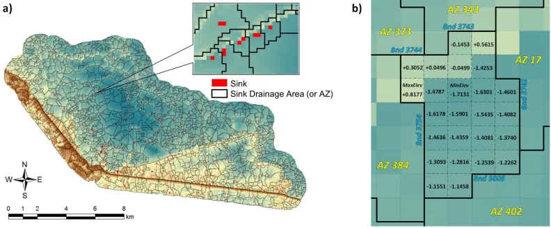
The output of the Sink Prescreening tool was, on the one hand, the “sink grid”, i.e. a map showing the preliminary 1355 sinks (whose drainage area respect the constrains imposed - see red cells in Figure 3a), and, on the other hand, a “pre-filled DEM”, i.e. a final DEM where the elevation of the 346 sinks was modified. More precisely, 1733 cells of the original Argenta DEM (corresponding to the 346 sinks) were filled: this elevation increment ranged between 0 and 3.26 m, with an average value equal to 0.16 m. As a consequence, the Argenta pre-filled DEM is substantially identical to the original DEM. It is worth pointing out that hereafter the pre-filled DEM substituted the original raw DEM in the subsequent steps of the pre-processing phase.
Finally, the sink drainage area identified by ArcHydro represents the AZs previously defined and shown in Figure 2. Overall the Argenta DEM was subdivided into 1355 AZs.
Sink Evaluation
Figure 3a shows the sink drainage areas, or AZs, associated to the 1355 prescreened sinks (in red) in the input Argenta pre-filled DEM and drawn in ArcGIS by the Sink Evaluation tool.
Figure 3b provides an example where all the attributes listed above are identified and represented for the accumulation zone AZ 380: as can be seen, its elevation ranges between MinElev and MaxElev, that are the elevation of the lowest and highest cell within the considered AZ, respectively. MinElev is of particular importance among these attributes because it represents the elevation of the AZ accumulation point.
Sink Selection
The Sink Selection function/tool is an interactive tool that allows the analyst to select sinks, and the associated AZ, desired. In practice, the user can specify particular conditions that the sink has to satisfy to be selected (together with the corresponding AZ), defining threshold values for some sink parameters like sink area, volume and sink drainage area. Previous evaluated sinks in the prefilled DEM with values greater than the specified values are selected and their attribute IsSink is set to 1. Otherwise this latter attribute is set to 0 and both the sink and the corresponding drainage area (or AZ) are not involved in the subsequent steps of the pre-processing analysis.
For Argenta case study, a composite criteria was made with the 3 aforesaid threshold values for sink parameters equal to 0: this implies that all the 1355 sinks (i.e. the 1355 AZs) previously evaluated satisfied all the criteria and were selected. This operation was an expedient to use all the AZs covering the Argenta terrain, avoiding the presence of “holes” in the calculation domain of the subsequent spreading phase. Therefore, this function was applied to correctly and automatically update the attribute IsSink of all the 1355 sinks, thus becoming input to the following pre-processing tools.
Drainage Area Characterization
The Drainage Area Characterization tool allows to generate the elevation-area-volume table (DrainEAV table) for each sink drainage area, i.e. for each AZ. In practice, each drainage area is subdivided in a fixed number of horizontal slices and information about elevation, cumulative area and volume are collected for each slice. In particular, for each slice the following attributes are calculated: BottomElev, bottom elevation of the slice, TopElev (top elevation of the slice), SlcElev (mid elevation of the slice, i.e. 0.5*(BottomElev+TopElev)), CumArea (area of the drainage area having an elevation that is less than or equal to TopElev), CumVolume (volume of water needed to fill the associated drainage area up to TopElev).
The input to this tool was the Argenta pre-filled DEM containing the elevation values, the Sink_DA feature class storing the 1355 AZs to characterize and the number of slices set to 10. The generated Argenta case study DrainEAV table listed the attributes of 14905 slices overall.
Drainage Boundary Definition
Starting from the pre-filled DEM and the corresponding array of sink drainage areas, this function generates a 3D-polyline for each boundary line between two drainage areas. This tool interpolates the elevation of the four closest cells surrounding the interpolation point along the boundary line and this information is stored the Boundary feature class. At the same time, the tool generates the Drainage connectivity table (DrainConn table) where the left and right catchments connected by each drainage boundary are stored (using their respective identification code). With specific reference to the Argenta case study, overall, 4013 polylines were identified and for each of them both the minimum and maximum elevation were gathered in the Boundary feature class. The minimum elevation along each boundary line is important because it is essential for the definition of the communication level of each AZ.
Drainage Boundary Characterization
width and area: BottomElev (bottom elevation of the slice), TopElev (top elevation of the slice), SlcElev (mid elevation of the slice, i.e. 0.5*(BottomElev+TopElev)), SlcWidth (width of water that covers the boundary line for the speciefied TopElev), SlcArea (cross-section area that is below the TopElev and above the BottomElev of the slice), CumArea (cross-section area that is below the TopElev), SlcPerimeter (wetted perimeter).
Figure 3: a) Division of Argenta DEM into AZs, b) example of sink drainage area attributes for the AZ 380.
Referring to the example in Figure 3b, the AZ 380 borders with other five AZs, thus its boundary consists of 5 boundary lines. With reference to each boundary line, the attributes of its corresponding slices were listed in the BndEWA table, as well as those of all the other lines of the study area.
As can be seen in the second row of Table 1, while the processing time associated to almost all the steps performed in ArcHydro has been kept below few minutes, the Drainage Area Characterization of 1355 sinks drainage areas in Argenta took a long time, about 8 hours, although spurious sinks had been preliminary reduced by using the Sink prescreening tool. In general, the greater the number of evaluated sinks, the more time consuming is the Drainage Area Characterization function.
3
The spreading phase
In the spreading phase of the RFSMs, the flood volume V is input into the flood-prone area at one or more points representing the places where the flood phenomenon originates. The temporal evolution of the flood phenomenon is completely disregarded and the hydraulic behaviour of the system of AZs is described through a sequence of “hydrostatic conditions”. Each “hydrostatic condition” represents a computational step in which the volume V is divided among neighbouring AZs on the basis of exchange mechanisms whereby the AZs are filled and the volumes exceeding their capacity spill over into adjacent AZs. The filling/exchange process ends when the volume stored in each of the AZs involved does not exceed its corresponding storage capacity.
RFSMunif model which assumes an instantaneous filling of the AZs inundated, (10) subdivide the volume V in the first input cell (and thus in all subsequent cells) into r parts in order to mimic the temporal dynamics of a flood: in other words, the various AZs are filled in successive steps, that is, a little at a time.
After characterizing in detail the Argenta terrain morphology through the terrain pre-processing phase described in Section 2, the geometric data generated in ArcGISTM environment (in particular the Sink_DA and Boundary feature classes, the DrainEAV, BndEWA and Drainconn tables) were duly organized and converted in txt files and, together with the AZ or AZs representing the starting “point” of the incoming flood volume V, formed the input for the “flood simulation” performed using MatlabTM.
The three RFSMs were applied to two case studies, varying the initial points (or AZs) where the water volume V, equal to 4.000.000 m3, is put into the Argenta area: they were chosen in such a way as to initially flood the AZs which lie adjacent to the river bank line and vary in size (AZ 918: large; AZ 673: medium).
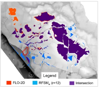
Figure 4: Flood maps: comparison between RFSMw (r = 12) and FLO-2D models.
Finally, the resulting flooded areas and depths were converted in raster format to compare them with those produced by the two-dimensional hydraulic model FLO-2DTM (16). In FLO-2D model a constant hydrograph (duration 10000 s for the two test cases) was defined as the initial condition and the Manning coefficient for the territory was set equal to 0.04 m-1/3s. Therefore, the flooded areas comparison and the RFSMs accuracy evaluation were made in ArcGISTM environment.
Regarding test case with the inlet AZ 673, overall all the RFSMs showed to perform well: in fact, the percentage error Bias in the flooded area estimate ranged between -20.2 and 2.5 % while the root-mean-square error RMSE of the depths over the whole Argenta area was kept below 0.20 m. The flood map produced by RFSMw (r =12) characterized by the lowest Bias (Bias = 0.5%) with respect to the wet areas produced by the FLO-2D model is shown in Figure 4.
The comparison between the computational times of the RFSMs (below 120 seconds) and that of the FLO-2D model (1.29E+06 seconds) demonstrated the significant increase in computational efficiency. This evidence shows the RFSMs’s suitability in flood risk analysis as they require only one preliminary pre-processing phase after which all the necessary flood simulations can be performed with extremely low calculation times.
4
Discussion and Conclusions
low computational times. It is worth noting that the application of these RFSMs necessarily requires a preliminary pre-processing phase aimed at characterizing in detail the terrain where the flood occurs. This study shows how is it possible to perform this preliminary terrain analysis in ArcGISTM environment through a manual sequence of ArcHydro tools designed to subdivide the ground into accumulation zones and to gather the geometrical information essential for the subsequent spreading phase.
Processing times of the RFSMs are dependent on a number of different factors: first, the extension of the flooded area and in fact the more extended and complex the investigated topography, the more time consuming is the stepwise approach of the terrain pre-processing phase; secondly, the number of software languages involved, since also the transformation of input data from a format to another takes time. In this study the initial ArcHydro geometric data are converted into txt files that are then read in MatlabTM environment to perform the flood simulation. Subsequently the resulting water depths are (re)stored in raster format to visualize the flood maps in ArcGISTM environment, thus coming back to the original environment.
In light of these considerations, further research is ongoing and in particular the substitution of the MatlabTM hydraulic phase with a code written in Python language directly embedded in ArcGISTM is under development. This would greatly simplify the RFSMs by eliminating the passage from one software to another and containing the overall processing times.
References
1. Normalised flood losses in Europe: 1970–2006. Barredo, J.I. 2009, Nat. Hazards Earth Syst. Sci., pp. 97-104.
2. Directive 2007/60/EC of the European Parliament and of the Council of 23 October 2007 on the assessment and management of flood risks. European Union. 2007, Off. J. Eur. Union L 288, pp. 27-34.
3. DHI Water & Environment. Hydrodynamic Module User Guide. 2009. 4. WL | Delft Hydraulics. SOBEK River/Estuary User Manual. 2005. 5. EDF-DRD. TELEMAC-2D Software Version 5.2 User Manual. 2002.
6. A non-hydrostatic pressure distribution solver for the nonlinear shallow water equations over irregular topography. Aricò, C. and Lo Re, C. 2016, Advances in Water Resources, pp. 47-69.
7. A weighted cellular automata 2D inundation model for rapid flood analysis. Guidolin, M., et al. 2016, Environmental Modelling & Software, pp. 378-394.
8. A methodology for regional-scale flood risk assessment. Gouldby, B., et al. 2008, Proceedings of the Institution of Civil Engineers - Water Management, pp. 169-182.
9. Recent development and application of a rapid flood spreading method. Lhomme, J., et al.
2009, Flood Risk Management: Research and Practice, pp. 15-24.
10. A rapid model for delimiting flooded area. Bernini, A. and Franchini, M. 2013, Water Resources Management, pp. 3825-3846.
11. ESRI. ArcHydro Tools for ArcGIS 10 - Tutorial. 2012.
12. Maidment, D.R. Arc Hydro: GIS for Water Resources. Redlands CA : Esri Press, 2002. 13. A DEM-based approach for large-scale floodplain mapping in ungauged watersheds.
Jafarzadegan, K. and Merwade, V. 2017, Journal of hydrology, pp. 650-662.
14. A framework model for the dimensioning and allocation of a detention basin system: The case of a flood-prone mountainous watershed. Bellu, A., et al. 2016, Journal of Hydrology, pp. 567-580.
15. Modeling the hydrologic effects of roadside ditch networks on receiving waters. Buchanan, B.P., et al. 2013, Journal of Hydrology, pp. 293-305.