Exploring the impact of Lean manufacturing on flexibility in SMEs

(1)

JIEM, 2017 – 10(5): 919-945 – Online ISSN: 2013-0953 – Print ISSN: 2013-8423 https://doi.org/10.3926/jiem.2119

Exploring the Impact of Lean Manufacturing on Flexibility in SMEs

Franco Lucherini , Mario Rapaccini

Università degli Studi di Firenze (Italy)

[email protected], [email protected]

Received: October 2016

Accepted: October 2017

Abstract:

Purpose: This paper describes the use of simulation and case-study research to assess flexibility gains induced by the adoption of three Lean Manufacturing practices.

Design/methodology/approach: We gather useful material and information about the manufacturing process of a selected Small-Medium Enterprise by adopting a case-research approach. The Value Stream Mapping is the method used for visualizing flows of products and information along the production system. Starting from the current arrangement of the company, computer simulation is used to assess the benefits arising from Cellular Manufacturing, Just-in-Time Delivery by Suppliers, and Single Minute Exchange of Dies.

Findings: To investigate the flexibility improvements coming from the introduction of Lean Manufacturing, we present a simulation model of the described company on which we performed our analysis. We quantify the flexibility of different configurations according to the new 5-step approach in order to segregate the contribution of different lean techniques.

(2)

mostly related to the provision of a supporting method for the decision making process propaedeutic to Lean Manufacturing introduction.

Keywords: lean manufacturing, manufacturing flexibility, case-study, simulation, SMEs, value stream mapping

1. Introduction

Previous research acknowledges that manufacturing firms can achieve significant improvements from the introduction of lean practices (Singh, Garg & Deshmukh, 2008; Thomas, Barton & Chuke-Okafor, 2008). Lean approaches are recommended to mitigate uncertainty, reduce costs and improve productivity (Boyle & Scherrer-Rathje, 2009).

Despite this relevance, there is paucity of studies specifically focused on lean applications to Small-Medium Enterprises (hereafter SMEs), and some authors claim for further research (Bakås, Govaert & van Landeghem, 2011; Shah & Ward, 2003). This paper aims at filling this gap. In particular, we address how the introduction of lean management practices can enhance manufacturing flexibility in SMEs.

By using computer simulation and a case-study we develop a staged approach to quantitatively assess the flexibility improvements induced by the introduction of three Lean Manufacturing practices. This complements existing studies that discuss the importance of Lean Manufacturing in SMEs solely from a qualitative perspective (Achanga, Shehab, Roy & Nelder, 2006; Rose, Deros, Rahman & Nordin, 2011; Zhou, 2016).

(3)

2. Literature Review

This work builds at the intersection of two major research fields, i.e. Manufacturing Flexibility and Lean Manufacturing. This section provides literature review and synthesis of the concepts that we consider relevant for the paper’s scope. In particular, we introduce Manufacturing Flexibility and a set of lean techniques used for its enhancement. Value Stream Mapping, and its combined use with computer simulation, is also presented since it is used to appraise the deliverables of Lean Manufacturing.

2.1. Manufacturing Flexibility (MF)

(4)

2.2. Lean Manufacturing (LM)

As well known, Lean Manufacturing (hereafter LM) was initially set up in the Japanese automotive industry as a new concept, in reaction to the serious circumstance of the post-world war II economy. Womack et al. (1990), in his seminal book, suggests a five-step approach aimed to ban waste and maximize the performances of production flows. LM techniques conceived for these purposes are widely discussed in the operations management literature (Feld, 2000; Monden, 2011; Nahmias, 2001). Hereafter, we review those applications that in our opinion can likely influence the MF performances.

• Cellular Manufacturing (hereafter CELLMFG). In CELLMFG the company’s production is structured into cells; these are defined as single working units, enclosing equipment and resources necessary to produce the highest number of similar products.

• Just-in-time Delivery by Suppliers (hereafter JITds). JITds ensures that suppliers deliver the right quantity at the right time in the right place (Shah & Ward, 2007). Ansari and Modarress in their work (Ansari & Modarress, 1988) state that the base of this technique is a partnership between the Supplier and the Company. Their study also confirms that JITds contributes to the improvement of product quality and productivity of each kind of company.

• Single Minute Exchange of Dies (hereafter SMED). Changing the production sequence from one product to another requires usually significant time for machines setup. SMED arises from the need to have a Quick Changeover. This procedure consists in converting as much as possible the IED (Inside Exchange of Die) in OED (Outside Exchange of Die), practically minimizing setup activities that require downtimes.

2.3. Value Stream Mapping (VSM)

(5)

and restructuring of the overall production process. Once completed, the method can start again as part of the systematic and continuous improvement process.

2.4. Simulation as Support to Value Stream Mapping

Since it is almost impossible to quantify the achievable gains in terms of KPI (i.e. the Work-in-process inventory) with a future state map only, simulation constitutes an appropriate complementary tool (McDonald, van Aken & Rentes, 2002). This solution to evaluate the profitability of an investment, that constitutes a base requirement for the financing of lean introduction (Sullivan, McDonald & van Aken, 2002), is usually cost effective and generally cheaper than a practical on the field test. Many examples of this approach combining VSM and simulations are available in literature (Abdulmalek & Rajgopal, 2007; Bernards, van Engelen, Schrauwen, Cramer & Luitjens, 1990; Gurumurthy & Kodali, 2011; Lian & van Landeghem, 2007; McDonald et al., 2002; Narasimhan, Parthasarathy & Narayan, 2007; Wang, Guinet, Belaidi & Besombes, 2009). One of the most popular simulation tools available on the internet is Arena Simulation (Detty & Yingling, 2000; Hammann & Markovitch, 1995; Kelton, 2002). This software has been selected for the present work considering that its diffusion is wide and that its features have been successfully proven in similar studies (Detty & Yingling, 2000; Lian & van Landeghem, 2002).

3. Research Methodology

A foundational case research provides the base data for the accomplishments of this paper. Then, computer simulation leverages that material to apprise the connections between LM and MF. Section 3 presents the main methods and tools adopted during this study.

3.1. Case Research (CR)

(6)

evidences (Lewis, 1998). According to Yin (2013), CR is an empirical exploration that aims to investigate a contemporary phenomenon in its real context. This happens especially when the boundaries between phenomenon and context are not clearly evident, and when multiple sources of evidence – such as field observations and interviews – are used. Thus, this strategy is recommended when the following criteria are fulfilled:

• Linkages between the phenomenon under examination and the context are not evident;

• Events cannot be reproduced in a laboratory;

• Events observation is possible;

• Typical research questions are of ‘how’ and ‘why’ types.

These criteria fit well with the aims of this work, as we investigate the correlations between LM and MF through field analysis of a case study.

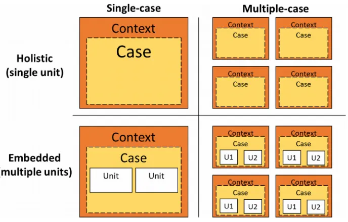
Literature discriminate case studies on the basis of two main parameters:

• The number of cases examined: single or multiple case-study.

• The aim of the study: holistic (single units of analysis) or embedded (multiple units of analysis).

Figure 1. Case Studies (Yin, 2013)

(7)

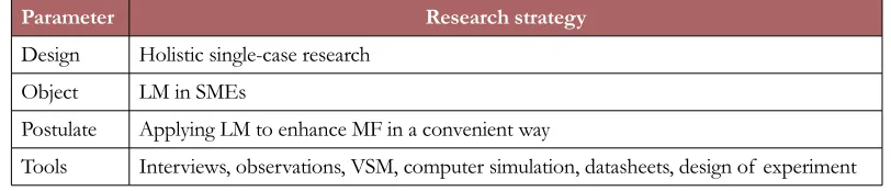
facility that cannot be molded into embedded subunits. On the base of the previous considerations, we set the outline of the research strategy used in this paper as presented in Table 1.

Parameter Research strategy

Design Holistic single-case research Object LM in SMEs

Postulate Applying LM to enhance MF in a convenient way

Tools Interviews, observations, VSM, computer simulation, datasheets, design of experiment

Table 1. Research strategy

The paper addresses the following research question:

How LM and MF are connected in the SME context.

We clarify the flexibility gains that are specifically due to the introduction of lean methods. We apply VSM in combination with the use of computer simulation to measure flexibility objectively. To this concern, we develop a set of metrics for the quantitative evaluation of performance improvement.

3.2. Computer Simulation (CS)

(8)

4. Case Study

As said, ALFA was purposively selected as this firm well fits in the paper’s scope due to the following reasons:

a) It is a small manufacturing company in a niche market, competing with medium- and big-sized rivals;

b) Managers indicate that flexibility is relevant for ALFA, but not easy to achieve since departments that are in charge of each stage of the manufacturing process often take their decisions in isolation;

c) Managers consider the capacity to adapt to the market a critical asset to be enhanced;

d) Managers declared they would have supported this study providing us with manifold, even confidential data.

4.1. Case Study Description

Since the ‘50s, the primary business of ALFA is the decoration of glassware by screen printing. In the beginning, ALFA mostly focused on the local market, but time after time it gained a good reputation for its crafting abilities that, in combination with cutting-edge technologies, make the difference in this kind of business. This is the reason why around 50% of revenues are currently from sales to foreign countries. In the last years, however, ALFA is facing a downtrend due to the unfavorable economic situation in the Italian consumer market. In addition, it is suffering the growing competition, especially on foreign markets, on which its shares are slightly but continuously reducing. As the overall sales decrease, the demand for customized products tends to increase. In sum, ALFA was typically looking for a way to obtain flexibility gains without raising its baseline costs (Madrid-Guijarro, García & van Auken, 2009; Rose et al., 2011). Managers agreed that LM could be the straightforward way towards this result.

4.2. Data Collection Methodologies

(9)

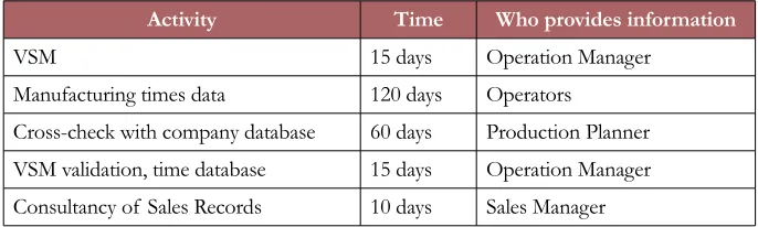
Table 2 summarizes the time we were engaged in field activities and provides an overview of the efforts required for future analysis of similar small-medium manufacturing facilities.

Activity Time Who provides information

VSM 15 days Operation Manager

Manufacturing times data 120 days Operators

Cross-check with company database 60 days Production Planner VSM validation, time database 15 days Operation Manager Consultancy of Sales Records 10 days Sales Manager

Table 2. Efforts and references of field activities

The next section describes how ALFA produces its products.

4.3. Manufacturing Process

(10)

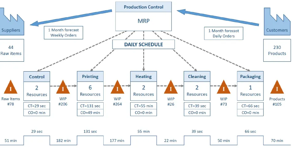
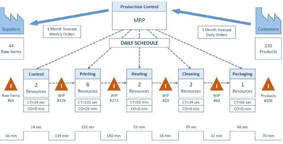
replenishing inventories of the factory outlet, which is close to the production facility. The described production flow has been mapped according to Rother and Shook (2003) and represented in Figure 2, that also shows the departments of the production facility.

Figure 2. VSM Design Point: #1 Current State Map

The current manufacturing performances of ALFA are summarized in Table 3:

Performance Parameters & Indicators Average Value

Production Level 9.0 Batches/day

Mix of products Random List

Total Cycle Time 611 min

Total Added Value Time 59 min

Total Change Over Time 49 min

Total WIP Inventory 751

Resources Utilization 61.0%

(11)

5. Simulations Analysis

To estimate the flexibility gains coming from the introduction of LM, we developed a simulation model of the described process, on which we performed our analysis. Assumptions and objectives of this simulation study are illustrated in the following section.

5.1. Predicted Performances

In this study, we simplify the model from Suarez, Cusumano, and Fine (Suarez, Cusumano & Fine, 1996), and focus on Volume Flexibility (hereafter VOLF) and Mix Flexibility (hereafter MIXF), that drive most of the overall MF (Hallgren & Olhager, 2009; Metternich, Böllhoff, Seifermann & Beck, 2013). To estimate and compare the flexibility performance of different manufacturing systems, we developed two process parameters that ease the characterization of Manufacturing Volume and Manufacturing Mix: Volume Indicator (hereafter VI, Equation 1), Mix Indicator (hereafter MI, Equation 2). To provide a proper definition of these indicators, the following parameters must be defined: CPL is the Current Production Level that the system is required to produce, namely the number of batches produced each day; MPC is the Maximum Productive Capacity that a given system arrangement can achieve assuming a random productive sequence; QIP is the average Quantity of Identical Products’ batches manufactured in series during the process.

(1)

(2)

In the current situation, the minimum acceptable level of production for ALFA is about the 50% of maximum capacity (VI = 50%) and the best optimization of the sequence is 2 identical lots in series (MI = 2).

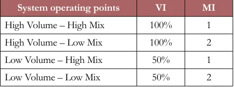
The vertices of the operating window, which are the extreme conditions of process parameters, are presented in Table 6.

System operating points VI MI

High Volume – High Mix 100% 1

High Volume – Low Mix 100% 2

Low Volume – High Mix 50% 1

Low Volume – Low Mix 50% 2

(12)

Building on these parameters, we measured the flexibility of different configurations according to the following 5-step approach shown in Figure 3 and described below.

Figure 3. 5-step Approach

Step 1. Calculation of maximum productive capacity

In the first step, we calculate the Maximum Productive Capacity (hereafter MPC) of the system via software. It represents the simulated capacity of the system reacting to the following inputs: immediate request of 30 batches of each product in the catalog; MI = 1. This value is strongly dependent upon the system configuration and defines the production levels for the next simulations. In facts, two levels of volume rate are tested with the software model: 100% and 50% of maximum capacity.

Step 2. Generation of the production sequences

The combination of different levels of VI and MI generates the 4 operating points declared in Table 6. We generate 4 production sequences based on each of these points to be used as input of the simulation models. The production sequences consist of 5 days of warm-up, actual simulation of 600 days (30 samples of 20 days).

Step 3. Simulation of the system

(13)

Step 4. Data collection

The software tracks and records the position of each products batch during the simulations. Similarly, the utilization of resources is documented. After that, a Visual Basic post processor automatically analyses the raw data in order to extrapolate key performance indicators.

Step 5. Evaluation on flexibility indicators

To quantitatively appraise flexibility vs. efficiency gains, we refer to commonly agreed measures (Bateman, 1999; Mendonça-Tachizawa & Giménez-Thomsen, 2007; Shah & Ward, 2003; Sohal, Keller & Fouad, 1989) such as:

(3)

Given a VI level, WIP is calculated as the average quantity of items stored in the production buffers during a 20 days’ simulation sample for MI = 1 and the equivalent sample for MI = 2.

(4)

Given a VI level, RU is defined as the average utilization of resources during a 20 days’ simulation sample for MI = 1 and the equivalent sample for MI = 2.

(5)

Given a MI level, PL is defined as the average production level achieved during a 20 days’ simulation sample for VI = 2. With reference to the definition of MPL provided above in Step 1, PL differs from MPC since it is evaluated for different MI and it is specific for a simulation sample. MPC on the contrary is a reference value for a system configuration and it is calculated for MI = 1.

The flexibility of the system is evaluated on 3 Responses, which are calculated through the indicators obtained in Step 5.

Capacity Response (hereafter CR): This response indicates the normalized difference between the maximum production achievable with an optimized sequence of products and a random list (Equation 6).

(14)

Considering a constant set of possible products, VOLF results in a function of fixed costs and production capacity only (Parker & Wirth, 1999). Hence, a production system is flexible when characterized by a constant and high production capacity, and operating with low fixed costs.

Inventory Response (hereafter IR): This response indicates the normalized difference between the inventory level at maximum production and the inventory level at half production (Equation 7).

(7)

Bartezzaghi and Turco confirm the connection between an overall low level of inventory with a MIXF oriented approach (Bartezzaghi & Turco, 1989). Thus, a stable and low work in progress inventories level can be considered as an additional estimator for the MIXF level.

Utilization Response (hereafter UR): This response indicates the difference between the resources utilization at maximum production and the resources utilization at half production (Equation 8).

(8)

The resource utilization of a rigid system decreases when the production volume drops since a part of the resources is not employed. On the contrary, in a flexible system, resources can be temporarily used for the completion of other activities during the downturn (Julie Yazici, 2005; Lee & Ebrahimpour, 1984), and an additional capacity can be outsourced during peaks of demand. Hence, a flexible system presents a steady and high level of resource utilization, regardless of the fluctuation in demand.

We assess the effects of lean techniques on flexibility completing the 5-step approach for all the investigated production layouts and comparing results.

5.2. Design of Experiment (DoE)

For the Design of Experiment (hereafter DoE), we adopt the L^k Factorial Design strategy (Law & Kelton, 2000) to simulate the ALFA’s manufacturing plant. With this method, we are able to efficiently study the correlation between performance and the structure of the system itself.

(15)

Design point SMED JITds CELLMFG

DP#1 As Is – – –

DP#2 SMED + – –

DP#3 JITds – + –

DP#4 SMED, JITds + + –

DP#5 CELLMFG – – +

DP#6 CELLMFG, SMED + – +

DP#7 CELLMFG, JITds – + +

DP#8 CELLMFG, SMED, JITds + + +

Table 4. Design Points

The adoption of the factors in Table 4 is commented below:

The SMED technique is interpreted in the context of this research as a method to reduce the setup time of the print stations, the setup time of the frames for the screen printing, and the required handlings for the controls of raw materials. The adoption of this technique is linked to the investments needed to modernize tools and equipment, currently used in the operations. Figure 4 shows the VSM updated considering a 50% reduction of times related to changeover and control activities. This value is in line with the expectation of ALFA’s management.

(16)

The performances of ALFA operating in the SMED configuration are summarized in Table 5:

WIP Inventory 692

Table 5. Manufacturing Performances of SMED configuration

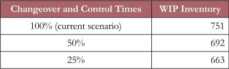
The data presented in Table 5 show a 7.9% decrease in WIP. The beneficial effect of SMED on inventory has been also evaluated with a different assumption: 75% decrease in changeover and control activities. In this case, the decrease in WIP is 11.7%.

Changeover and Control Times WIP Inventory

100% (current scenario) 751

50% 692

25% 663

Table 6. SMED effect on inventory

(17)

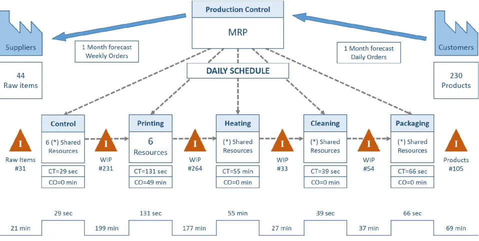
Figure 5. VSM Design Point: #3 JITds Map

The performances of ALFA operating in the JITds configuration are summarized in Table 7:

WIP Inventory 539

Table 7. Manufacturing Performances of JITds configuration

(18)

Figure 6. VSM Design Point: #5 CELLMFG Map

The performances of ALFA operating in the CELLMFG configuration, with 12 operators instead of 13, are summarized in Table 8:

WIP Inventory 717

(19)

5.3. Case Study Results

This section discusses the findings from our simulation experiments with respect to the research question presented in section 3.1.

How LM and MF are connected in the SME context.

We find that LM techniques have different impacts on the operational performance of the plant. These effects are quantified in Table 9.

Technique Effect on CR Effect on IR Effect on UR

Avg. Std. Dev. Avg. Std. Dev. Avg. Std. Dev.

SMED (1.6%) 0.3% (19.85) 29.73 0.2% 1.2%

JITds (0.1%) 0.0% (31.19) 10.94 0.0% 1.1%

CELLMFG (1.0%) 0.1% (58.60) 19.42 33.1% 1.2%

Table 9. Summary of Effects

Looking at the first columns in Table 5 the effect on CR, is evident for all techniques – CR Avg. values are all negatives and, in absolute value, 1.6% for SMED, 0,1% for JITds, and 1.0% for CELLMFG –. SMED, as expected, is the most useful. In fact, the setup times are the necessary No Added Value operations, which mostly penalize the flexibility in this context.

With reference to the effect on IR, the analysis on differences between the WIP at 100% and at 50% capacity is statistically complex because of the high fluctuation of the inventory itself (very high standard deviations are associated with the metrics). Due to the high reductions of the parameters, it is anyway clear that the contribution of JITds and CELLMFG to the maintaining of an inventory level, adequate to the production level is positive – IR Avg. values are all negatives and, in absolute value, 31.19% for JITds, and 58.60% for CELLMFG –. In particular, JITds seems to be the most effective technique, able also to reduce the variability in WIP.

(20)

According to the obtained responses data, LM can be considered a good strategy to increase MF as it contributes to equalize the system performances under varying boundary conditions (production mix or volume).

The present study shows that the benefits achieved by the use of SMED, JITds, and CELLMFG have strong implications also on the flexibility of production systems.

For instance, reducing the setup time by using SMED, the ratio between the value-added operations and the overall cycle time increases. Consequently, the general improvements obtainable in this case study through the Single Minute Exchange of Die are a 7% increase in production. The decrease in tooling is particularly important when a high Mix Flexibility is required. Moreover, the simulation shows that the difference in productivity between a low-mix and a high-mix scenario drops from the 37% of the basic arrangement to the 35% of the SMED configuration. Based on this, the SMED can be considered a good solution for manufacturing systems where the production of batches with variable size is required. The higher is the investment on these techniques, the higher are the percentage benefits.

The Just-in-Time is commonly used for a general reduction of the inventory. The analysis of the company ALFA shows that a daily supply of raw materials produces a high level of WIP. Simulating an advanced replenishing logic by JITds, the stock levels drop significantly – about 30% –. The reduction in inventory is more pronounced when the level of production, and therefore the daily storage of raw materials, is high (Perceptual decrease is almost constant). This phenomenon contributes to flatten the WIP stock, and, thus, increases the Volume Flexibility.

(21)

6. Conclusions

This study investigates the connections between Lean Manufacturing and Manufacturing Flexibility within the Small-Medium Enterprise context. Case Research is used to fill the need for experiential evidences about lean introduction into small companies (Bakås et al., 2011; Moeuf et al., 2016). In that regard, the cause effect relationship between lean techniques and flexibility enhancement is explored in an uncommon field. A single case approach is leveraged to obtain a detailed analysis and a better view on this topic (Burgess, 1993; Crotty, 1998; Voss et al., 2002).

On this basis, the first novel contribution of this research is the gathering of empirical data about the use of Lean for Flexibility improvement in a small firm. The present work focuses on two types of flexibility that are commonly deemed the most important (Hallgren & Olhager, 2009; Metternich et al., 2013): MIXF and VOLF. On the basis of the available literature about the above mentioned flexibilities (Bartezzaghi & Turco, 1989; Bateman, 1999; Mendonça-Tachizawa & Giménez-Thomsen, 2007; Parker & Wirth, 1999; Sohal et al., 1989), the following KPIs have been selected for their measurement: Production Capability, Inventory Level, and Resource Utilization. Single Minute Exchange of Die, Just in Time delivery by Suppliers and Cellular Manufacturing are the lean techniques focused upon this paper. The flexibility gains for the company have been evaluated by simulations. Single Minute Exchange of Die produces an improved and stable Production Capability, which entails an enhancement of VOLF; this benefit is particularly remarkable when a high product mix is also needed. Just in Time delivery by Suppliers reduces the Inventory Level, improving the MIXF. Cellular Manufacturing generates a positive effect on Resource Utilization, producing lower fixed costs; this enhances the VOLF, and, indirectly, has a positive effect on the MIXF by harmonizing the inventory levels. Although specific benefits vary from case to case, it can be said that the operational process of lean thinking contributes to the competitiveness of the firm under examination.

(22)

The principal limitation of this study is the low generalizability of the results which are related to a single case study. In spite of the solidity of this limitation, one of the deliverables of the work is a method for the collection of additional experimental evidences. In this regard, the next possible step of this work should be a comparison between additional samples, that would also allow the optimization of the system and its full automation in a dedicated software tool. Considering this, an in-depth study with other case researches would be desirable for the further extension of the operation management research field.

References

Abdulmalek, F.A., & Rajgopal, J. (2007). Analyzing the benefits of lean manufacturing and value stream mapping via simulation: A process sector case study. International Journal of production economics, 107(1), 223-236. https://doi.org/10.1016/j.ijpe.2006.09.009

Abernethy, M.A., & Lillis, A.M. (1995). The impact of manufacturing flexibility on management control system design. Accounting, Organizations and Society, 20(4), 241-258.

https://doi.org/10.1016/0361-3682(94)E0014-L

Achanga, P., Shehab, E., Roy, R., & Nelder, G. (2006). Critical success factors for lean implementation within SMEs. Journal of Manufacturing Technology Management, 17(4), 460-471.

https://doi.org/10.1108/17410380610662889

Ansari, A., & Modarress, B. (1988). JIT purchasing as a quality and productivity centre. The International Journal of Production Research, 26(1), 19-26. https://doi.org/10.1080/00207548808947838

Bakås, O., Govaert, T., & van Landeghem, H. (2011). Challenges and success factors for implementation of lean manufacturing in European SMES. Paper presented at the 13th International conference on the Modern Information Technology in the Innovation Processes of the Industrial Enterprise (MITIP).

Bartezzaghi, E., & Turco, F. (1989). The impact of just-in-time on production system performance: An analytical framework. International Journal of Operations & Production Management, 9(8), 40-62.

https://doi.org/10.1108/EUM0000000001257

Bateman, N. (1999). Measuring the mix response flexibility of manufacturing systems. International Journal of Production Research, 37(4), 871-880. https://doi.org/10.1080/002075499191571

(23)

Bernards, J., van Engelen, G., Schrauwen, C., Cramer, H., & Luitjens, S. (1990). Simulation of the recording process with a VSM on Co-Cr and Co-Ni-O layers deposited at oblique incidence. IEEE Transactions on Magnetics, 26(5), 2289-2291. https://doi.org/10.1109/20.104700

Boyle, T.A., & Scherrer-Rathje, M. (2009). An empirical examination of the best practices to ensure manufacturing flexibility: Lean alignment. Journal of Manufacturing Technology Management, 20(3), 348-366.

https://doi.org/10.1108/17410380910936792

Burgess, R.G. (1993). Research methods. Nelson.

Buzacott, J.A., & Mandelbaum, M. (1985). Flexibility and productivity in manufacturing systems. Paper presented at the Proceedings of the annual IIE Conference.

Cagliano, R., Blackmon, K., & Voss, C. (2001). Small firms under MICROSCOPE: International differences in production/operations management practices and performance. Integrated Manufacturing Systems, 12(7), 469-482. https://doi.org/10.1108/EUM0000000006229

Carpinetti, L.C., Gerolamo, M.C., & Dorta, M. (2000). A conceptual framework for deployment of strategy-related continuous improvements. The TQM Magazine, 12(5), 340-349.

https://doi.org/10.1108/09544780010341950

Crotty, M. (1998). The foundations of social research: Meaning and perspective in the research process. Sage.

Detty, R.B., & Yingling, J.C. (2000). Quantifying benefits of conversion to lean manufacturing with discrete event simulation: A case study. International Journal of Production Research, 38(2), 429-445.

https://doi.org/10.1080/002075400189509

Feld, W.M. (2000). Lean manufacturing: Tools, techniques, and how to use them. CRC Press.

https://doi.org/10.1201/9781420025538

Gerwin, D. (1993). Manufacturing flexibility: A strategic perspective. Management science, 39(4), 395-410.

https://doi.org/10.1287/mnsc.39.4.395

Gupta, Y.P., & Goyal, S. (1989). Flexibility of manufacturing systems: Concepts and measurements. European journal of operational research, 43(2), 119-135. https://doi.org/10.1016/0377-2217(89)90206-3

Gurumurthy, A., & Kodali, R. (2011). Design of lean manufacturing systems using value stream mapping with simulation: A case study. Journal of Manufacturing Technology Management, 22(4), 444-473.

(24)

Hallgren, M., & Olhager, J. (2009). Flexibility configurations: Empirical analysis of volume and product mix flexibility. Omega, 37(4), 746-756. https://doi.org/10.1016/j.omega.2008.07.004

Hammann, J.E., & Markovitch, N.A. (1995). Introduction to Arena [simulation software]. Paper presented at the Simulation Conference Proceedings. Winter. https://doi.org/10.1109/WSC.1995.478785

Hayes, R.H., & Pisano, G.P. (1994). Beyond world-class: The new manufacturing strategy. Harvard business review, 72(1), 77-86.

Jeong, K.-Y., & Phillips, D.T. (2011). Application of a concept development process to evaluate process layout designs using value stream mapping and simulation. Journal of Industrial Engineering and Management, 4(2), 206-230. https://doi.org/10.3926/jiem.2011.v4n2.p206-230

Julie-Yazici, H. (2005). Influence of flexibilities on manufacturing cells for faster delivery using simulation. Journal of Manufacturing Technology Management, 16(8), 825-841.

https://doi.org/10.1108/17410380510627843

Kelton, W.D. (2002). Simulation with ARENA. McGraw-Hill.

Law, A.M., & Kelton, W.D. (2000). Simulation modeling and analysis. McGraw-Hill.

Lee, S.M., & Ebrahimpour, M. (1984). Just-in-time production system: Some requirements for implementation. International Journal of operations & production management, 4(4), 3-15.

https://doi.org/10.1108/eb054721

Lewis, M.W. (1998). Iterative triangulation: A theory development process using existing case studies. Journal of Operations Management, 16(4), 455-469. https://doi.org/10.1016/S0272-6963(98)00024-2

Lian, Y.-H., & van Landeghem, H. (2002). An application of simulation and value stream mapping in lean manufacturing. Paper presented at the Proceedings 14th European Simulation Symposium.

Lian, Y.-H., & van Landeghem, H. (2007). Analysing the effects of Lean manufacturing using a value stream mapping-based simulation generator. International Journal of Production Research, 45(13), 3037-3058.

https://doi.org/10.1080/00207540600791590

Madrid-Guijarro, A., García, D. & van Auken, H. (2009). Barriers to innovation among Spanish manufacturing SMEs. Journal of Small Business Management, 47(4), 465-488.

https://doi.org/10.1111/j.1540-627X.2009.00279.x

(25)

Mascarenhas, M.B. (1981). Planning for flexibility. Long Range Planning, 14(5), 78-82.

https://doi.org/10.1016/0024-6301(81)90011-X

McDonald, T., van Aken, E.M., & Rentes, A.F. (2002). Utilising simulation to enhance value stream mapping: A manufacturing case application. International Journal of Logistics, 5(2), 213-232.

https://doi.org/10.1080/13675560210148696

Mendonça-Tachizawa, E., & Giménez-Thomsen, C. (2007). Drivers and sources of supply flexibility: An exploratory study. International Journal of Operations & Production Management, 27(10), 1115-1136.

https://doi.org/10.1108/01443570710820657

Metternich, J., Böllhoff, J., Seifermann, S., & Beck, S. (2013). Volume and mix flexibility evaluation of lean production systems. Procedia CIRP, 9, 79-84. https://doi.org/10.1016/j.procir.2013.06.172

Moeuf, A., Tamayo, S., Lamouri, S., Pellerin, R., & Lelievre, A. (2016). Strengths and weaknesses of small and medium sized enterprises regarding the implementation of lean manufacturing. IFAC-PapersOnLine, 49(12), 71-76. https://doi.org/10.1016/j.ifacol.2016.07.552

Monden, Y. (2011). Toyota production system: An integrated approach to just-in-time. CRC Press.

Nahmias, S. (2001). Production and Operations Analysis. Irwin, New York: McGraw-Hill.

Narasimhan, J., Parthasarathy, L., & Narayan, P.S. (2007). Increasing the effectiveness of value stream mapping using simulation tools in engine test operations. Paper presented at the 18th IASTED International Conference on Modeling and Simulation.

Nemetz, P.L., & Fry, L.W. (1988). Flexible manufacturing organizations: Implications for strategy formulation and organization design. Academy of Management Review, 13(4), 627-639.

Ohno, T. (1988). Toyota production system: Beyond large-scale production. CRC Press.

Parker, R.P., & Wirth, A. (1999). Manufacturing flexibility: Measures and relationships. European journal of operational research, 118(3), 429-449. https://doi.org/10.1016/S0377-2217(98)00314-2

Rose, A., Deros, B.M., Rahman, M.A., & Nordin, N. (2011). Lean manufacturing best practices in SMEs. Paper presented at the Proceedings of the 2011 International Conference on Industrial Engineering and Operations Management.

(26)

Shah, R., & Ward, P.T. (2003). Lean manufacturing: Context, practice bundles, and performance. Journal of operations management, 21(2), 129-149. https://doi.org/10.1016/S0272-6963(02)00108-0

Shah, R., & Ward, P.T. (2007). Defining and developing measures of lean production. Journal of operations management, 25(4), 785-805. https://doi.org/10.1016/j.jom.2007.01.019

Singh, R.K., Garg, S.K., & Deshmukh, S. (2008). Strategy development by SMEs for competitiveness: A review. Benchmarking: An International Journal, 15(5), 525-547. https://doi.org/10.1108/14635770810903132

Slagmulder, R., & Bruggeman, W. (1992). Investment justification of flexible manufacturing technologies: Inferences from field research. International Journal of Operations & Production Management, 12(7/8), 168-186. https://doi.org/10.1108/EUM0000000001310

Sohal, A., Keller, A., & Fouad, R. (1989). A review of literature relating to JIT. International Journal of Operations & Production Management, 9(3), 15-25. https://doi.org/10.1108/EUM0000000001228

Suarez, F.F., Cusumano, M.A., & Fine, C.H. (1996). An empirical study of manufacturing flexibility in printed circuit board assembly. Operations research, 44(1), 223-240. https://doi.org/10.1287/opre.44.1.223

Sullivan, W.G., McDonald, T.N., & van Aken, E.M. (2002). Equipment replacement decisions and lean manufacturing. Robotics and Computer-Integrated Manufacturing, 18(3), 255-265.

https://doi.org/10.1016/S0736-5845(02)00016-9

Thomas, A., Barton, R., & Chuke-Okafor, C. (2008). Applying lean six sigma in a small engineering company–a model for change. Journal of Manufacturing Technology Management, 20(1), 113-129.

https://doi.org/10.1108/17410380910925433

Vassell, C. (1999). Computer integrated manufacturing, and small and medium enterprises. Computers & industrial engineering, 37(1-2), 425-428. https://doi.org/10.1016/S0360-8352(99)00109-6

Vokurka, R.J., & O’Leary-Kelly, S.W. (2000). A review of empirical research on manufacturing flexibility. Journal of operations management, 18(4), 485-501. https://doi.org/10.1016/S0272-6963(00)00031-0

Voss, C., Tsikriktsis, N., & Frohlich, M. (2002). Case research in operations management. International journal of operations & production management, 22(2), 195-219. https://doi.org/10.1108/01443570210414329

Wang, T., Guinet, A., Belaidi, A., & Besombes, B. (2009). Modelling and simulation of emergency services with ARIS and Arena. Case study: The emergency department of Saint Joseph and Saint Luc Hospital. Production Planning and Control, 20(6), 484-495. https://doi.org/10.1080/09537280902938605

(27)

Xia, W., & Sun, J. (2013). Simulation guided value stream mapping and lean improvement: A case study of a tubular machining facility. Journal of Industrial Engineering and Management, 6(2), 456.

https://doi.org/10.3926/jiem.532

Yin, R.K. (2013). Case study research: Design and methods. Sage Publications.

Zhou, B. (2016). Lean principles, practices, and impacts: A study on small and medium-sized enterprises (SMEs). Annals of Operations Research, 241(1-2), 457-474. https://doi.org/10.1007/s10479-012-1177-3

Journal of Industrial Engineering and Management, 2017 (www.jiem.org)

Article’s contents are provided on an Attribution-Non Commercial 3.0 Creative commons license. Readers are allowed to copy, distribute and communicate article’s contents, provided the author’s and Journal of Industrial Engineering and Management’s