Online Appendix: Entry into Export Markets
1
Data
All the firms in our sample have Chile as country of origin and we restrict our analysis to firms whose main activity is the manufacture of chemicals and chemical products (ISIC sector number 24). This is the second largest export manufacturing sector in Chile. Our data set includes both exporters and non-exporters from 1995 to 2005. However, we restrict our sample to firms that have been active in Chile for all eleven years between 1995 and 2005.
Our data come from two separate sources. The first is an extract of the Chilean customs database, which covers the universe of exports of Chilean firms. The second is the Chilean Annual Industrial Survey (Encuesta Nacional Industrial Anual, or ENIA), which includes all manufacturing plants with at least ten workers. We merge these two data sets using firm identifiers, allowing us to exploit information on the export destinations of each firm and on their domestic activity. These two datasets provide us with information on the value exported per firm and destination country and the firm characteristics that we use to predict the actual revenue from exporting.1
We complement our customs-ENIA data with a database of country characteristics from CEPII.2 This database gives us information on the physical distance between any country and Chile, as well as on the gravity variables that we include inXictR. Finally, we collect data on real GDP per capita from the World Bank World Development Indicators.
2
Revenue Regression
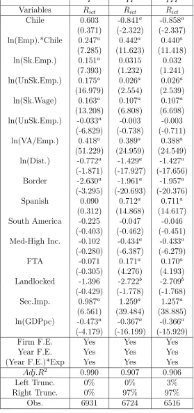
In the revenue regression, the observed right hand side covariate vector, XictR, includes:3 (a) firm characteristics: number of skilled and unskilled workers (Sk.Emp and UnSk.Emp), av-erage wage of skilled and unskilled workers (Sk.Wage and UnSk.Wage), and average value added per worker (VA/Emp); (b) country characteristics: dummy for being landlocked ( Land-locked), country-specific level of imports in chemical sector (Sec.Imp.), and GDP per capita (GDPpc); (c) gravity variables or distance measures: physical distance between Chile and destination country (Dist.), dummy for having a FTA with Chile (FTA), and dummies for sharing border (Border), continent (South America), language (Spanish), and World Bank GDP per capita group with Chile (Med-High Inc.). In addition, we introduce firm and year fixed effects, and allow a dummy capturing that country c is equal to Chile to change by year. We check the robustness of our results to outliers by running three separate regressions: regression I includes all the observed export flows; regression II drops the largest 3%; and regressionIII drops both the smallest and largest 3%.
We estimate the parameter vectorθusing Nonlinear Least Squares (NLLS). The estimates ofθ are contained in the following table.
1An observation in this data is a firm-country-year combination. For each observation we have
information on the value of goods sold in US dollars. We obtain sales values in year 2000 terms using the US CPI.
2Available at http://www.cepii.fr/anglaisgraph/bdd/distances.htm. Mayer and Zignago
(2006) provide a detailed explanation of the content of this database.
Table 1: Revenue Regression
I II III
Variables Rict Rict Rict
Chile 0.603 -0.841a -0.858a
(0.371) (-2.322) (-2.337) ln(Emp).*Chile 0.247a 0.442a 0.440a
(7.285) (11.623) (11.418)
ln(Sk.Emp.) 0.151a 0.0315 0.032
(7.393) (1.232) (1.241)
ln(UnSk.Emp.) 0.175a 0.026a 0.026a
(16.979) (2.554) (2.539)
ln(Sk.Wage) 0.163a 0.107a 0.107a
(13.208) (6.808) (6.698)
ln(UnSk.Emp.) -0.033a -0.003 -0.003 (-6.829) (-0.738) (-0.711) ln(VA/Emp.) 0.418a 0.389a 0.388a
(51.229) (24.959) (24.549) ln(Dist.) -0.772a -1.429a -1.427a
(-1.871) (-17.927) (-17.656) Border -2.630a -1.961a -1.957a
(-3.295) (-20.693) (-20.376)
Spanish 0.090 0.712a 0.711a
(0.312) (14.868) (14.617)
South America -0.225 -0.047 -0.046 (-0.403) (-0.462) (-0.451) Med-High Inc. -0.102 -0.434a -0.433a
(-0.280) (-6.387) (-6.279)
FTA -0.071 0.171a 0.170a
(-0.305) (4.276) (4.193)
Landlocked -1.396 -2.722b -2.709b (-0.429) (-1.778) (-1.768) Sec.Imp. 0.987a 1.259a 1.257a
(6.561) (39.484) (38.885)
ln(GDPpc) -0.473a -0.367a -0.366a (-4.179) (-16.199) (-15.929)
Firm F.E. Yes Yes Yes
Year F.E. Yes Yes Yes
(Year F.E.)*Exp Yes Yes Yes
Adj.R2 0.990 0.907 0.906
Left Trunc. 0% 0% 3%
In order to estimate the numbers in Table 1, we exclusively use data for those observa-tions with positive exports. Therefore, the estimated vector ˆθ verifies the following mean independence condition
E[Rict−r(XictR; ˆθ)|XictR,dict= 1] =E[νictR +εRict+ηRict|XictR,dict= 1] = 0,
where ηictR = r(XictR;θ) − r(XictR; ˆθ). Given that dict is potentially a function of νictR, the
estimate ˆθ will generally not be a consistent estimate of θ. More precisely, ˆθ is a consistent estimator ofθ if and only if
E[Rict−r(XictR;θ)|XictR,dict = 1] = 0, (1)
This moment condition will hold if (a)νR
ict = 0; and, (b)E[εRict|XictR] = 0.4
Even in those cases in which ˆθ is not a consistent estimator of θ, we can still consider
r(XictR,θˆ) as a reduced form approximation of the potential revenue from exporting,Rict, and,
moreover, as a proxy for the expected revenue from exporting,R∗ict. The resulting error term from using ˆRict =r(XictR,θˆ) as a proxy forR∗ict is
R∗ict−Rˆict =R∗ict−r(XictR,θˆ) =R
∗
ict−Rict+Rict−r(XictR,θˆ),
and it holds thatE
R∗ict−Rict|Jit
= 0 and E
Rict−r(XictR,θˆ)|XictR,dict = 1
= 0. The first orthogonality condition arises from the definition ofR∗ict as the expected revenue conditional on the information setJit. The second orthogonality condition is a direct implication of the
definition of ˆθ as the result of projecting realized revenues Rict on the nonlinear function r(XR
ict,θˆ).
3
Instrument Functions for Empirical Exercise
We present the results for three different sets of instruments. Remember from the main text that the vectorXict contains the proxy ˆRict that we use for the unobserved expected revenue
R∗ict. The vector Z1ict contains the distance covariateDc, measured without error, and the variable Z2ict incorporates the lagged revenue ˆRict−1 as an instrument for current revenue.
The vectorZict is defined as (Z1ict, Z2ict).
The first set of instruments incorporates the following six instruments:
Ψ(1)r (Xict, Z1ict) =
ˆ
Rict
1
Dc
−
ˆ
Rict
1
Dc
, Ψ(1)s (Xict, Z1ict) =
ˆ
Rict
1
Dc
λ(Xict, Z1ict)
−
ˆ
Rict
1
Dc
λ(Xict, Z1ict)
(2)
4A sufficient condition for restriction (b) is that XR
ict ∈ Jit. Note that we have not imposed this restriction so far and that it is not necessary;XR
where Ψ(1)r (·) is the set of instruments that we apply to the revealed preference inequalities,
Ψ(1)s (·) is the set applied to the score function inequalities,
λ(Xict, Z1ict) = fν(−uict(Xict, Z1ict;β))
Fν(−uict(Xict, Z1ict;β)),
and uict(Xict, Z1ict;β) = β1Rˆict−β2−β3Dc. The set of instruments in equation (2) defines
inequalities that contain the true value of the parameter vectorβ only under the assumption of no expectational error (i.e. perfect foresight). This set of instruments Ψ(1)(·) generates identified parameters that are identical to those arising from maximizing the log likelihood function:
L=E
L(Xict, Z1ict,dict)
=
E
dictlog 1−Fν(−uict(Xict, Z1ict;β))
+ (1−dict) log Fν(−uict(Xict, Z1ict;β))
. (3)
In order to prove that our moment inequalities, combined with the instrument vector in equation (2), identify the same parameter value as the maximum likelihood estimator, we show that these moment inequalities are equivalent to the first order condition from the maximization of the log likelihood function. In particular, the vectoral first order condition from maximizing the log likelihood function in equation (3) is:
E
ˆ
Rict
1
Dc
· h
dict
fν(−uict(Xict, Z1ict;β))
1−Fν(−uict(Xict, Z1ict;β))−(1−dict)
fν(−uict(Xict, Z1ict;β))
Fν(−uict(Xict, Z1ict;β))
i !
=
E
ˆ
Rict
1
Dc
·
hfν(−uict(Xict, Z1ict;β)) Fν(−uict(Xict, Z1ict;β)) i
·hdict
Fν(−uict(Xict, Z1ict;β)) 1−Fν(−uict(Xict, Z1ict;β))
−(1−dict) i
!
= 0
and this first order condition is equivalent to the combination of the following two inequalities:
E
ˆ
Rict
1
Dc
·
hfν(−uict(Xict, Z1ict;β)) Fν(−uict(Xict, Z1ict;β))
i ·hdict
Fν(−uict(Xict, Z1ict;β))
1−Fν(−uict(Xict, Z1ict;β))−(1−dict)
i !
≥0,
−E
ˆ
Rict
1
Dc
·
hfν(−uict(Xict, Z1ict;β)) Fν(−uict(Xict, Z1ict;β))
i ·hdict
Fν(−uict(Xict, Z1ict;β))
1−Fν(−uict(Xict, Z1ict;β))−(1−dict)
i !
≥0,
We can rewrite these two inequalities as
E Ψ(1)s (Xict, Z1ict)
h
dict
Fν(−uict(Xict, Z1ict;β)) 1−Fν(−uict(Xict, Z1ict;β))
−(1−dict) i
! ≥0,
The second set of instruments is:
Ψ(2)r (Zict) = ˆ
Rict−1
1
Dc
1/Dc
1/√Dc − ˆ
Rict−1
1
Dc
1/Dc
1/√Dc
, Ψ(2)s (Zict) = ˆ
Rict−1
1
Dc
1/Dc
1/√Dc
·λ(Zict)
− ˆ
Rict−1
1
Dc
1/Dc
1/√Dc
·λ(Zict) , (4)
where Ψ(2)r (·) is the set of instruments that we apply to the revealed preference inequalities,
Ψ(2)s (·) is the set applied to the score function inequalities,
λ(Zict) =
fν(−uict(Zict;β)) Fν(−uict(Zict;β)),
anduict(Zict;β) =β1Rˆict−1−β2−β3Dc.
The third set of instruments simply expands the second set to incorporate interaction terms of lagged revenues and distance:
Ψ(3)r (Zict) =
Ψ(2)s (Zict)
ˆ
Rict−1(1/Dc)
ˆ
Rict−1(1/ √
Dc)
−
ˆ
Rict−1(1/Dc)
ˆ
Rict−1(1/ √ Dc)
, Ψ(3)s (Zict) =
Ψ(2)s (Zict)
ˆ
Rict−1(1/Dc)
ˆ
Rict−1(1/ √
Dc)
·λ(Zict)
−
ˆ
Rict−1(1/Dc)
ˆ
Rict−1(1/ √
Dc)
·λ(Zict) . (5)
Both the second and third set of instruments are a function ofZ2ict = ˆRict−1 (instead ofXict
= ˆRict). Therefore, they are both consistent with the presence of expectational error and will