Market Efficiency of Commercial Bank in Financial Crisis

(1)

Issues

ISSN: 2146-4138

available at http: www.econjournals.com

International Journal of Economics and Financial Issues, 2016, 6(2), 756-764.

Market Efficiency of Commercial Bank in Financial Crisis

Han-Ching Huang

1

**_{*, Yong-Chern Su}**

2

_{, Tze-Yi Lin}

3

1_{Department of Finance, Chung Yuan Christian University, Taoyuan, 32023 Taiwan,}2_{Department of Finance, National Taiwan} University, Taiwan, 3_{Department of Finance, National Taiwan University, Taiwan. *Email: samprass@cycu.edu.tw}

ABSTRACT

This study investigates commercial bank market efficiency in financial crisis. We employ a time-varying generalized autoregressive conditional heteroskedasticity (GARCH) model because volatility matters in financial crisis. The empirical results show a significant positive relation between contemporaneous order imbalances and returns in convergence process toward efficiency. A direct linkage between volatility and order imbalances is examined by GARCH model. Surprisingly, a low connection exists between order imbalance and price volatility, implying that market makers are capable of mitigating commercial bank prices volatility in financial crisis. We develop an imbalance based trading strategy but fail to beat the market. A nested causality approach, which examines the dynamic return-order imbalance relationship during the price formation process, confirms the results.

Keywords: Order Imbalance, Market Efficiency, Commercial Bank, Financial Crisis

JEL Classifications: G01, G14, G21

1. INTRODUCTION

The global financial crisis has led to renewed criticism of the efficient-market hypothesis (EMH). As one prominent example, market strategist Jeremy Grantham has stated that

EMH is responsible for the current financial crisis and claim that belief in the EMH caused financial leaders to have a “chronic

underestimation of the dangers of asset bubbles breaking”1_. Renowned financial journalist and best-selling author Roger Lowenstein blasted the theory, stating “The upside of the current

Great Recession is that it could drive a stake through the heart of the academic nostrum known as the EMH”2_.

The main purpose of our study is to investigate market efficiency in 2008 financial crisis in the U.S., which is the leading and most efficient stock market in the world. Therefore, the magnitude of effect is far greater than 1997 financial crisis. We especially focus

1 Cited in a widely read New York Times business column, Joe Nocera, “Poking Holes in a Theory on Markets,” New York Times, June 5, 2009. http://www. nytimes.com/2009/06/06/business/06nocera.html?scp=1&sq=efficient%20 market&st=cse. See also Grantham’s foreword in Andrew Smithers, Wall Street Revalued: Imperfect Markets and Inept Central Bankers (Chichester, UK: Wiley, 2009).

2 On Wall Street, the Price isn’t Right.” Washington Post. 7 June, 2008.

on market efficiency of commercial banks. Beginning in the 1980s,

players in the U.S. mortgage market started to transfer the risk to other players, and some of these players are commercial banks, where customers deposit their money into checking or savings accounts. Commercial banks are also lending institutions. They provide mortgages and other types of loans to their customers, and in some cases pass these mortgages to other institutions. These mortgages are bundled into securities and sold to large investment banks and the government-sponsored entities Fannie Mae and Freddie Mac to get mortgage debt off their books. In this way, commercial banks have the capacity to make more loans.

Besides, commercial banks have an incentive to seek low-risk assets to meet the capital adequacy requirements which were set forth by the Basel Committee on Banking Regulation.

Commercial banks not only look for low-risk assets, but also seek assets that produce high yields on their investment to increase

profit. Commercial banks in the U.S. and worldwide thus have

an incentive to purchase assets that entail little risk and do not

require them to keep large amounts of capital on hand. Through securitization, the U.S. investment banks and other financial

institutions pool many different types of assets, including risky

subprime mortgages, to make assets “safer” and thus attract

(2)

in subprime mortgage-backed securities to get a greater yield for the same amount of risk.

However, during financial crisis period, these “safer” assets

became toxic assets that banks were no longer able to value and that were worth so little on the market. Thus, they have become

virtually un-sellable when credit rating agencies realized that the

assets they had rated as AAA, or very low-risk, were actually much riskier. Furthermore, according to mark-to-market accounting

rules, commercial banks are required to value mortgage backed securities and collateralized debt obligation based on their market

price, but banks were no longer able to value them accurately because there was no way of determining their risk. Those that are able to sell their assets on the market made a great loss because

the market prices of those assets were much lower than the assets’

original values. Since these assets were sold for such a low price, commercial banks that did not sell their assets had to lower the

value of, or “write down,” the assets on their balance sheets in order to “mark to market.” These write-downs hurt banks even

when they were not planning to sell the assets.

We can infer that there would be a large impact on commercial banks in financial crisis since these banks have toxic assets. Thus,

we observe the relation between order imbalances and returns to investigate whether informed traders have more inside information such as how many toxic assets commercial banks have and how

many debts are removed from balance sheet through securitization

process, and then they are able to get abnormal return.

There are some researches on stock market efficiency in 1997 financial crisis. Hoque et al., (2007) investigate the weak-form efficiency of eight Asian stock markets by adopting variance ration tests for the pre-crisis (1990-1997) and post-crisis (1998-2004) periods. They indicate that the crisis does not have significant effect on the efficiency degree, and six of the Asian markets continue inefficient after the crisis, while Korea has the opposite result. Taiwan market is the only one that gets improvement in efficiency

from the pre-crisis to post-crisis period. Jae and Shamsuddin

(2008) find that there is no significant change in the degree of market efficiency by using multiple variance ratio tests. Lim et al. (2006) conjecture that the nonlinear serial dependency structure is

attributed to unexpected shocks. They argue that investors were

swamped by panic, and this adversely affected the market’s ability to price stock efficiently. Cheong et al. (2007) separate the sample

data into four periods, that is, pre-crisis, crisis, USD pegged, and

post-crisis period. Their study shows that the highest inefficiency

is during the crisis period, followed by pre-crisis, post crisis, and

USD pegged period. Lim et al. (2008) investigate eight Asian stock markets’ efficiency in the 1997 financial crisis for pre-crisis,

crisis, and post-crisis periods by using the rolling bi-correlation test statistic. Their result presents that the crisis badly affected the

efficiency of most Asian stock markets, with Hong Kong being strike severely, yet most of these markets’ efficiency get improved

in the post-crisis period. They also indicate that investors would overreact not only to local news, but also news from other markets, particularly adverse news. Moreover, Choudhry and Jayasekera

(2015) examine twenty five UK firms of different sizes and from different industries from 2004 to 2010, which includes the current

global financial crisis. They find that most firms and industries seem to support the market efficiency hypothesis during good

periods (booms) and bad periods (recessions). However, the level

of market efficiency seems to decline significantly from the pre-crisis to pre-crisis period. Both the results of market efficiency and declining market efficiency from the pre-crisis to crisis periods support the asymmetric effect of the financial crisis on the beta of UK firms.

In brief, most of previous studies about efficiency in financial crisis show that market cannot achieve efficiency during market crash

period. Moreover, some researchers observe the trading volume or order imbalances to investigate the behavior of informed traders and examine whether there exists information asymmetry.

In our study, we use order imbalance to investigate relations among intraday stock return, volatility and order imbalances of

commercial banks during financial crisis. We choose short event window in order to minimize the noise arising from random

price movements and errors owing to misestimates of benchmark

returns. Chordia et al. (2002) find that the order imbalances are

strongly related to past market returns and are strongly related to contemporaneous absolute returns after controlling for market

volume and market liquidity. Order imbalance increases (decrease)

after market declining (rising), which shows that investors are contrarians on aggregate. However, either excess buyer- or

seller-initiated order imbalances reduces liquidity. Moreover,

order imbalances affect market returns even after controlling for

aggregate volume and liquidity. Guillermo et al. (2002) adopt a

simple model, in which the investors trade for two reasons which is to share risk or to speculate upon private information. They argue that the relation between current returns, volume, and future returns

depends on the relative significance of speculative trade versus hedging trade. They find that returns generated by speculative

trades tend to continue themselves, while returns generated by hedging trades tend to reverse themselves. Moreover, they also

find that smaller firms with higher bid-ask spread tend to maintain

their returns following high volume.

Chordia and Subrahmanyam (2004) test the relation between

order imbalances and daily returns of individual stocks. They

find that contemporaneous imbalances are strongly related to

contemporaneous returns, but the positive relation between lagged imbalance and returns disappears after controlling for the contemporaneous imbalances. In addition, individual stock order

imbalances are strongly and auto-correlated. Chordia et al. (2005)

provide the relation between order imbalances and stock returns

for different intervals. They find that order imbalances are highly

positively dependent over both short and long time intervals. They

argue that market can achieve weak-form efficiency between 5

and 6 min.

In our study, we don’t find a significant positive relation between

current stock returns and lagged-one order imbalances. The

empirical results show that within 10 or 15 min interval, market makers adjust inventories to mitigate volatility. We separate overall

effect, auto-correlated effect, and cross-correlated effect. In overall

(3)

order imbalances is observed, and this result is contrary to cross-correlated effect situation. The contemporaneous order imbalances

are significantly positive for all time intervals at 1% level, while most of the coefficients of lagged-one imbalances turn to be significantly negative, which is consistent with Chordia and Subrahmanyam (2004). We also document a convergence process

from 5 min interval to 15 min interval. Our trading strategies are not capable of beating the market.

Our study proceeds as follows. Section 2 describes data.

Section 3 presents the return-order imbalances relation. We discuss the dynamic return (volatility)-order imbalance generalized

autoregressive conditional heteroskedasticity (GARCH) relation in

Section 4. Section 5 shows the market efficiency testing through an imbalance-based trading strategy. We exhibit Dynamic causal

relationship in explaining the return-order imbalance relationship in Section 6, and Section 7 concludes.

2. DATA

Major U.S. commercial banks are included in our samples.

We observe commercial bank efficiency from September 9 to September 18, 2008, namely 4 days before and after Lehman Brothers bankruptcy. We collect intraday transactions data from

Trade and Quote (TAQ).

Stock are included or excluded depending on the following

criteria. First, the firm must be included in both the Compustat and TAQ database. Second, the top four commercial banks (Bank of America, Wells Fargo, City Bank, and American Express) are listed in NYSE based on liquidity and size concern. Third, we delete transactions within the first 90 s after the opening of the market to avoid noise trading. Fourth, quotes established and transactions

traded before the opening or after the close are excluded.

3. RETURN-ORDER IMBALANCES

RELATION

We apply Lee and Ready (1991) trade assignment algorithm on intraday returns and order imbalances for 5-, 10-, and 15-min time intervals. We use a multi-regression to examine the impact of five lagged order imbalances on current stock returns for three

different time intervals.

R_t = α₀+α₁OI_t₋₁+α₂OI_t₋₂+α₃OI_t₋₃+α₄OI_t₋₄+α₅OI_t₋₅+ε_t (1)

Where R_t is the current stock return of the individual stock. OI_t_−i

are the lagged order imbalances at time t−1, t−2, t−3, t−4, and t−5

of the sample stocks.

An imbalance-based trading strategy is developed on the condition

that order imbalances have a significant impact on return. We also

include contemporaneous and four lagged order imbalances to examine conditional lagged return- order imbalance regression relation for three time intervals. According to Chordia and

Subrahmanyam (2004), we expect a positive relation between

contemporaneous imbalances and current returns, and a negative relation between current returns and lagged order imbalances after controlling for the contemporaneous order imbalances because of information over-weighting of market makers. Moreover, we observe how market makers dynamically accommodate the imbalances pressure by examining whether there is a trend among

three different time intervals (5-, 10-, 15-min).

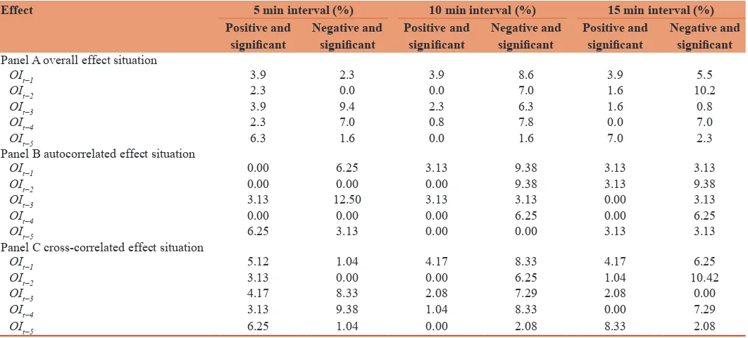
Table 1 presents the percentages of positive and significant

coefficients of lagged-one order imbalance are 3.9%, 3.9%, and 3.9% in 5-, 10-, and 15-min intervals respectively. From Panel A, we observe that the percentage of positive and significant of lagged-one order imbalance is higher than negative and significant

Table 1: Empirical results of unconditional lagged return-order imbalance relation

Effect 5 min interval (%) 10 min interval (%) 15 min interval (%)

Positive and

significant Negative and significant Positive and significant Negative and significant Positive and significant Negative and significant

Panel A overall effect situation

OIt−1 3.9 2.3 3.9 8.6 3.9 5.5

OIt−2 2.3 0.0 0.0 7.0 1.6 10.2

OIt−3 3.9 9.4 2.3 6.3 1.6 0.8

OIt−4 2.3 7.0 0.8 7.8 0.0 7.0

OI_t−5 6.3 1.6 0.0 1.6 7.0 2.3

Panel B autocorrelated effect situation

OIt−1 0.00 6.25 3.13 9.38 3.13 3.13

OI_t−2 0.00 0.00 0.00 9.38 3.13 9.38

OI_t−3 3.13 12.50 3.13 3.13 0.00 3.13

OIt−4 0.00 0.00 0.00 6.25 0.00 6.25

OIt−5 6.25 3.13 0.00 0.00 3.13 3.13

Panel C cross-correlated effect situation

OIt−1 5.12 1.04 4.17 8.33 4.17 6.25

OIt−2 3.13 0.00 0.00 6.25 1.04 10.42

OIt−3 4.17 8.33 2.08 7.29 2.08 0.00

OIt−4 3.13 9.38 1.04 8.33 0.00 7.29

OIt−5 6.25 1.04 0.00 2.08 8.33 2.08

Rt=α0+α1OIt−1+α2OIt−2+α3OIt−3+α4OIt−4+α5OIt−5+εt. Where Rt is the stock return at time t of the sample stock, OIt is the lagged order imbalances at time t of the sample stocks, εt is the

(4)

one in 5 min interval, but both are insignificant. Surprisingly, significantly negative lagged-one imbalance is much larger then positive in 10 min interval at 10% and 5% significant level and in 15 min interval at 10% significant level. This finding can be explained as follows. When negative information shock occurs during financial crisis, informed traders eager to short stocks.

They herd or spread their orders out over time, which causes a huge negative order imbalance. Confronted with the imbalance

pressure, market makers react against that by reducing the quote

price within 5 min interval, and the lower price does mitigate the

pressure of selling for a while. We infer that within 10 min interval

or 15 min interval would be a better interval for market makers

to adjust inventories. Therefore, they raise quote prices and cause positive 10 min and 15 min returns, which leads to a negative

relation between lagged-one imbalance and returns.

In addition, we find that the percentage of negative and significant

lagged-three imbalances is relatively high in comparison with that of other lagged imbalances under 5 min interval. It implies that market makers are not able to determine whether the large order imbalance is caused by informed traders or not. Thus, they wait

for two periods to confirm and start to adjust quote price back to

normal level. Moreover, except for lagged-one and lagged-two

imbalances under 5 min interval, the percentage of all significantly

negative lagged imbalances are much larger than positive one in other lagged order imbalances, indicating that they tend to

adjust quote price back to normal level gradually to offload their

inventory rather than to correct at a stroke after they react by

lowering or raising quote price in the beginning.

Panel B summarizes the empirical results of return on its own order imbalance at 5% significant level. The ratios of positive and significant coefficients of lagged-one order imbalance are 0%, 3.13%, and 3.13% under 5-, 10-, and 15-min intervals

respectively. In contrast to the result of previous overall effect, the

ratio of significantly negative lagged-one imbalance is larger than positive one under 5 min interval at 10% and 5% significant level, which is inconsistent with Chordia and Subrahmanyam (2004). It indicates that market makers react immediately and efficiently at the moment confronted with auto order imbalances. We presume

that market makers know private information before shock arrives

in financial crisis period, and market makers had already prepared

enough inventories to accommodate order imbalance shocks.

Panel C illustrates findings of returns on order imbalances from other stocks, namely cross effect at 5% significant level. The percentages of positively significant coefficients of lagged-one order imbalance are 5.21%, 4.17%, and 4.17% under 5-, 10-, and

15-min intervals respectively. The result of cross-correlated effect

is similar to overall effect. Andrade et al. (2008) explain that a

demand shock for only one stock affects prices of other stocks

due to the hedging desires of liquidity providers. In Panel C, the ratio of significantly positive coefficient of lagged-one imbalance

is larger than negative one, which is contradict to auto-correlated effect. The possible explanation is as follows. Market makers,

as liquidity providers, execute buy orders if they meet other stocks’ buy orders from other traders for liquidity and hedging

concerns just as what is mentioned above. They tend to raise

quote price to induce other traders to sell in order to maintain

their inventory level. Therefore, demand shock from other stock

induce market makers to raise quote price of the individual stock,

thus bring about positive relation between returns and lagged -one imbalances.

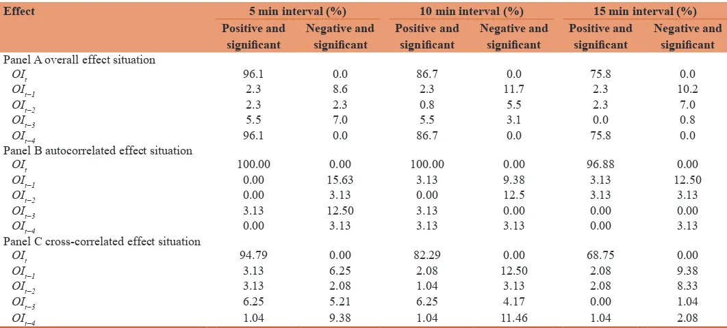
Table 2 presents that contemporaneous order imbalances are

significantly positive at all significant levels and under all time

intervals in overall effect, auto-correlated effect, and

cross-correlated effect situation, while most of the coefficients of

Table 2: Empirical results of conditional contemporaneous return-order imbalance relation

Effect 5 min interval (%) 10 min interval (%) 15 min interval (%)

Positive and

significant Negative and significant Positive and significant Negative and significant Positive and significant Negative and significant

Panel A overall effect situation

OIt 96.1 0.0 86.7 0.0 75.8 0.0

OIt−1 2.3 8.6 2.3 11.7 2.3 10.2

OIt−2 2.3 2.3 0.8 5.5 2.3 7.0

OIt−3 5.5 7.0 5.5 3.1 0.0 0.8

OI_t−4 96.1 0.0 86.7 0.0 75.8 0.0

Panel B autocorrelated effect situation

OIt 100.00 0.00 100.00 0.00 96.88 0.00

OI_t−1 0.00 15.63 3.13 9.38 3.13 12.50

OI_t−2 0.00 3.13 0.00 12.5 3.13 3.13

OIt−3 3.13 12.50 3.13 0.00 0.00 0.00

OIt−4 0.00 3.13 3.13 3.13 0.00 3.13

Panel C cross-correlated effect situation

OIt 94.79 0.00 82.29 0.00 68.75 0.00

OIt−1 3.13 6.25 2.08 12.50 2.08 9.38

OIt−2 3.13 2.08 1.04 3.13 2.08 8.33

OIt−3 6.25 5.21 6.25 4.17 0.00 1.04

OIt−4 1.04 9.38 1.04 11.46 1.04 2.08

Rt=α0+α1OIt−1+α2OIt−2+α3OIt−3+α4OIt−4+α5OIt−5+εt. Where Rt is the stock return at time t of the sample stock, OIt is the lagged order imbalances at time t of the sample stocks, εt is the

(5)

lagged-one imbalances turn to be significantly negative, which is consistent with Chordia and Subrahmanyam (2004). They argue

that the positive relation between lagged imbalances and returns disappears after controlling for the current imbalance. Market makers overweight the impact of current trades which are

auto-correlated with past trades, as a consequence they reverse the quote

price to offset the overreaction in next period.

From Panels B and Panel C of Table 2, we find that the result of

auto-correlated and cross-correlated effect are similar. It implies that in these two conditions, market makers have concern for information contained in order imbalances and inventory risk. Nonetheless, the magnitude is larger in auto-correlated effect because market makers tend to adjust inventory level by degree of correlation of stocks, and correlation in cross-correlated effect is lower than that of individual stock.

4. DYNAMIC RETURN

(VOLATILITY)

-

ORDER IMBALANCE

GARCH RELATION

In order to explore the impact of volatility on return-order

imbalance relation, we adopt a time-varying GARCH model. We

use the model to examine the dynamic relation between returns and order imbalances under three different time intervals (5 min,

10 min, and 15 min):

R_t= α +βOI_t+ε_t

ε_t|Ω_t₋₁~N(0,h_t)

h_t = +A Bh_t₋₁+Cε_t2₋₁ (2)

Where R_tis the return at time t, and is defined as lnP_t-lnP_t₋₁. OI_t

denotes the explanatory variable of order imbalance. β is the coefficient describing the impact of order imbalance on stock returns. ε_tis the residual value of the stock return at time t. h_tis conditional variance at time t. Ω_t₋₁ is the information set in at time t−1.

Intuitively, a large order imbalance is positively associated with a

large volatility. We expect a significant positive β. Furthermore, we

examine how long it takes for commercial bank market to achieve

efficiency. Therefore, we adopt a GARCH model to investigate

whether a larger order imbalances lead to a larger price volatility under three different time intervals.

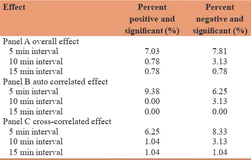
The empirical results of dynamic return-order imbalance GARCH relation have been presented in Table 3. In contrast with the results in the above regression models, there exists a clear convergence

process. At 5% significant level, the proportion of significantly positive β are 71.88%, 43.75%, and 28.13% under 5-, 10-,

and 15-min interval respectively in auto-correlated effect, and

51.04%, 35.42%, and 18.75% under 5-, 10-, and 15-min interval

respectively in cross-correlated effect. From the empirical

findings, we confirm the important role of volatility on

return-order imbalance relation.

The relation between price volatility and order imbalance is also

an important issue in our study. We expect that there is a positive

correlation between price volatility and order imbalances, that is, large price volatility is accompanied by large order imbalances. The results are presented in Table 4.

We observe that the proportion of significantly positive or negative coefficients of order imbalances is not as large as we expect,

indicating that the impact of order imbalance on volatility is not

as strong as we expect. At 5% significant level, the proportion of significantly positive β are 9.38%, 0%, and 0% under 5-, 10-, and 15-min interval respectively in auto-correlated effect, and 6.25%, 1.04%, and 1.04% under 5-, 10-, and 15-min interval respectively

in cross-correlated effect. The low connection between order imbalances and price volatility could be explained that market

makers show the capability of mitigating commercial banks’ price volatility in financial crisis.

Table 3: Empirical results of the dynamic return-order imbalance GARCH (1, 1) relation

Effect Percent

positive and significant (%)

Percent

negative and significant (%)

Panel A overall effect

5 min interval 56.25 0.78

Panel B auto correlated effect

Panel C cross-correlated effect

Rt=α+βOIt+εt, εt|Ωt−1~N(0, ht), ht= +A Bht−1+Ct−1 2

ε Where Rt is the return at time t, and

defined as ln(Pt)-ln(Pt−1), OIt denotes the explanatory variable of order imbalance, β is the coefficient describing the impact of order imbalance on stock returns, ht is the

conditional variance at time t, Ωt−1 is the information set in at time t−1. “Significant”

denotes significant at the 5% level

Table 4: Empirical results of the dynamic volatility-order imbalance GARCH (1, 1) relation

Effect Percent

positive and significant (%)

Percent

negative and significant (%)

Panel A overall effect

Panel B auto correlated effect

Panel C cross-correlated effect

Where Rt is the return at time t, and is defined as ln(Pt)-ln(Pt−1), OIt denotes the

explanatory variable of order imbalance. ε_t is the residual value of the stock return at

time t. ht is the conditional variance at time t, Ωt−1 is the information set in at time t, γ is

(6)

5. MARKET EFFICIENCY TESTING

THROUGH AN IMBALANCE BASED

TRADING STRATEGY

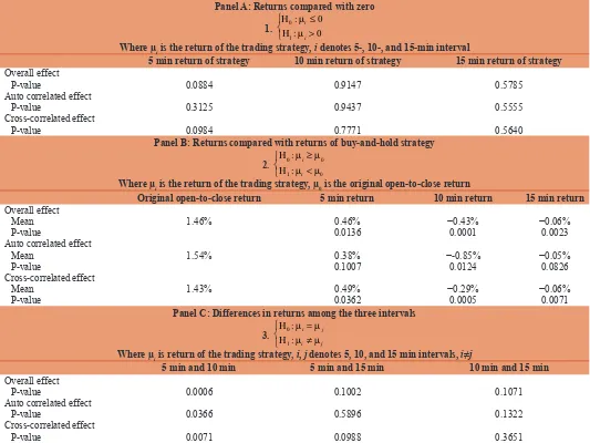
We take a further step to test market efficiency through an intraday imbalance based trading strategy. We truncate 10% of the largest order imbalance to trade under 5-, 10-, and 15-min interval. We

buy when positive order imbalance appears, and short when it turns negative. The results are presented in Table 5.

Panel B shows that we earn a daily return of 0.38%, −0.85%, and −0.05% under 5-, 10-, and 15-min interval respectively in auto-correlated effect; 0.49%, −0.29%, −0.06% under 5-, 10-,

and 15-min interval respectively in cross-correlated effect. The returns in cross-correlated effect seem to be higher than those of auto-correlated effect. A one-tail Z-test has been performed. The

P-values reported in Panel A are 0.3125, 0.9437, 0.5555 under 5-, 10-, and 15-min interval respectively in auto-correlated effect, and 0.0984, 0.7771, and 0.5640 under 5-, 10-, and 10-min interval respectively in cross-correlated effect. At 5% significant level, there is no significant positive profit by executing the trading strategy.

We also perform paired-t test to test whether the trading strategy

can beat the market, that is, original open-to-close return. From

Panel B, we find that the one-tail P-values are 0.1007, 0.1241, and 0.0826 under 5-, 10-, and 15-min interval respectively in auto-correlated effect, and 0.0362, 0.0004, and 0.0071 under 5-, 10-, and 15-min interval respectively in cross-correlated effect. We can’t argue the trading strategy beat the market in either

auto-correlated or cross-auto-correlated effect.

In addition, we check whether the trading strategy makes

significantly difference among 5-, 10-, and 15-min intervals. Panel C shows that the returns of strategy under 5-min interval are significantly better than those under 10-min interval in both

auto-correlated effect and cross-correlated effect situation, but

insignificant difference.

To sum up, we find that imbalance-based trading strategy is not able to beat the market in commercial banks in financial crisis, which implies that there exists an efficient market. Moreover, we get the result that 5-min returns of strategy are significantly better than 10-min returns, and this is consistent with our

previous empirical results of dynamic return-order imbalance

Table 5: Trading profit

Panel A: Returns compared with zero

1. HH

0

1

0

0 :

:

µ µ

i

≤ >   

Where µi is the return of the trading strategy, i denotes 5-, 10-, and 15-min interval

5 min return of strategy 10 min return of strategy 15 min return of strategy

Overall effect

P-value 0.0884 0.9147 0.5785

Auto correlated effect

P-value 0.3125 0.9437 0.5555

Cross-correlated effect

P-value 0.0984 0.7771 0.5640

Panel B: Returns compared with returns of buy-and-hold strategy

2. HH

0 0

1 0

:

µ µ

i

≥ <   

Where µ_i is the return of the trading strategy, µ₀ is the original open-to-close return

Original open-to-close return 5 min return 10 min return 15 min return Overall effect

Mean 1.46% 0.46% −0.43% −0.06%

P-value 0.0136 0.0001 0.0023

Mean 1.54% 0.38% −-0.85% −0.05%

P-value 0.1007 0.0124 0.0826

Mean 1.43% 0.49% −0.29% −0.06%

P-value 0.0362 0.0005 0.0071

Panel C: Differences in returns among the three intervals

3. HH

0

1

:

µ µ

i j

= ≠   

Where µ_i is return of the trading strategy, i, j denotes 5, 10, and 15 min intervals, i≠j

5 min and 10 min 5 min and 15 min 10 min and 15 min

Overall effect

P-value 0.0006 0.1002 0.1071

P-value 0.0366 0.5896 0.1322

(7)

GARCH relation, which shows a decreasing trend from 5-min

to 10-min interval. Thus, market makers do have the capability

of mitigating volatility through inventory adjustments, even in

financial crisis.

6. DYNAMIC CAUSAL RELATIONSHIP

IN EXPLAINING THE RETURN-ORDER

IMBALANCE RELATIONSHIP

Finally, in order to explain the story behind an imbalance-based trading strategy, we employ a nested causality to explore the dynamic causal relationship between returns and order imbalances.

According to Chen and Wu (1999), we define four relationships

between two random variables, x₁and x₂, in terms of constraints on the conditional variances of x_1(T+1) and x_2(T+1)based on various available information sets, where x_i=(x_i1, x_i2., x_iT), i=1, 2, are vectors of observations up to time period T.

Definition 1: Independency, x₁˄x₂:

x₁and x₂are independent if:

Var x( ₍_T ₎ x) Var x( _T x x, ) Var x( _T x x x, ,

~ ( ) ~ ~ ( ) ~ ~ (

1 +1 1 = 1 +1 1 2 = 1 +1 1 2 2TT+1)

~ )

(3)

And

Var x( (T ) x ) Var x( T x x, ) Var x( T x x x, ,

~ ( ) ~ ~ ( ) ~ ~ (

2 +1 2 = 2 +1 1 2 = 2 +1 1 2 1TT+1)

~ )

(4)

Definition 2: Contemporaneous relationship, x₁ <−> x₂:

x₁ and x₂are contemporaneously related if:

Var x( ₍_T ₎ x) Var x( _T x x, )

~

( )

~ ~

1 +1 1 = 1 +1 1 2 (5)

Var x( ₍_T ₎ x x, ) Var x( _T x x x, , _T )

~ ~

( )

~ ~

( )

~

1 +1 1 2 > 1 +1 1 2 2 +1 (6)

And

Var x( _T x ) Var x( _T x x, )

( ) ~

( ) ~ ~ 2 +1 2 = 2 +1 1 2

(7)

Var x( ₍_T ₎ x x, ) Var x( _T x x x, , _T )

~ ~

( )

~ ~

( )

~

2 +1 1 2 > 2 +1 1 2 1 +1 (8)

Definition 3: Unidirectional relationship, x₁=>x₂:

There is a unidirectional relationship from x₁to x₂if:

Var x( (T ) x) Var x( T x x, )

~

( )

~ ~

1 +1 1 = 1 +1 1 2 (9)

And

Var x( ₍_T ₎ x ) Var x( _T x x, )

~

( )

~ ~

2 +1 2 > 2 +1 1 2 (10)

Definition 4: Feedback relationship, x₁<=>x₂:

There is a feedback relationship between x₁ and x₂if

Var x( (T ) x) Var x( T x x, )

~

( ) ~ ~ 1 +1 1 > 1 +1 1 2

(11)

And

Var x( _T x ) Var x( _T x x, )

( ) ~

( ) ~ ~ 2 +1 2 > 2 +1 1 2

(12)

To explore the dynamic relationship within a bi-variate system, we

form the five statistical hypotheses in Table 6 where the necessary

and sufficient conditions corresponding to each hypothesis are

given in terms of constraints on the parameter values of the vector autoregression (VAR) model. To determine whether there

exists a specific causal relationship, we use a systematic multiple

hypotheses testing method.

The causal relationships are defined as follows: ˄ represents

independency; <−> is the contemporaneous relationship; ≠> is the negation of a unidirectional relationship; <=>is the feedback

relationship; ≠>> is the negation of a strong unidirectional relationship where σ₁₂=σ₂₁=0; and <<=>> is a strong feedback relationship where σ₁₂=σ₂₁=0.

Unlike the traditional pair-wise hypothesis testing approach, this testing method avoids the potential bias induced by restricting the causal relationship to a single alternative hypothesis. To implement this method, we employ the results of several pair-wise hypothesis tests. For instance, in order to conclude that x₁=>x₂, we need to establish that x₁<≠x₂and to reject that x₁≠>x₂. To conclude that

x₁<−>x₂, we need to establish that x₁<≠x₂as well as x₁≠>x₂and also to reject x₁˄x₂. In other words, it is necessary to examine all

five hypotheses in a systematic way before we draw the conclusion

that a dynamic relationship exists. The following presents an

Table 6: Hypotheses on the dynamic relationship of a bivariate system

Hypotheses The VAR test

H₁: x₁^x₂ φ₁₂ (L)=φ₂₁ (L)=0, and σ₁₂=σ₂₁=0 H₂: x₁<−>x₂ φ₁₂ (L)=φ₂₁ (L)=0

H₃: x₁≠>x₂ φ₂₁ (L)=0

H₃*: x₂≠>x₁ φ₁₂ (L)=0

H₄: x₁<=>x₂ φ₁₂ (L)* φ₂₁ (L) ≠0 H₅: x₁≠>>x₂ φ₂₁ (L)=0 , and σ₁₂=σ₂₁=0 H₆: x₂≠>>x₁ φ₁₂ (L)=0 , and σ₁₂=σ₂₁=0 H₇: x₁<<=>>x₂ φ₁₂ (L)* φ₂₁ (L) ≠0 , and σ₁₂=σ₂₁=0

The bivariate VAR model may be expressed as: 11 12

21 22 ϕ ϕ ϕ ϕ ( ) ( ) ( ) ( ) L L L L           1 2 t t x x        = 1 2 t t ε ε       

 where x1t and

x2t are mean adjusted variables. The first and second moments of the error structure,

~

( , ) '

ε ε εt= 1t 2t are that, E t( ) ~

ε =0 and

E t t k( )

~ ~

ε ε+ =0for k≠0 and _{E t t k}( )

~ ~

ε ε+ = Σfor k=0,

where Σ =

(8)

inference procedure that starts from a pair of the most general alternative hypotheses.

Our inference procedure for exploring the dynamic relationship is based on the principle that a hypothesis should not be rejected

unless there is sufficient evidence against it. In the causality

literature, most tests intend to discriminate between independency and an alternative hypothesis. The primary purpose of the literature cited above is to reject the independency hypothesis. On the contrary, we intend to identify the nature of the relationship

between two financial series. The procedure consists of four testing sequences, which implement a total of six tests (denoted

as a-f), where each test examines a pair of hypotheses. The four

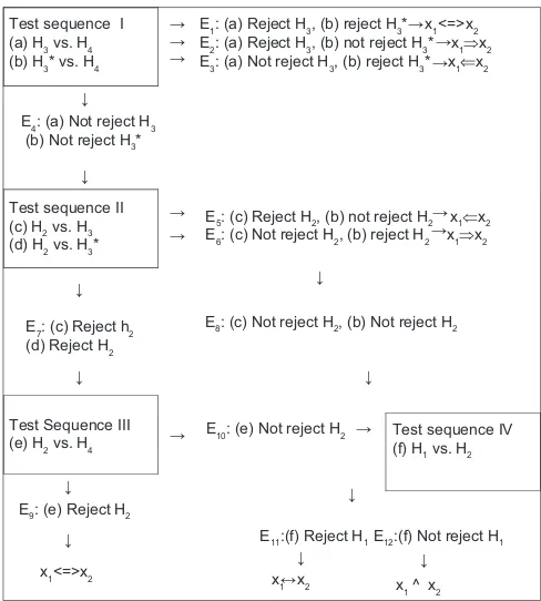
testing sequences and six tests are summarized in a decision-tree flow chart in Figure 1.

To explore the dynamic return-order imbalance relationship during the price formation process, we employ a nested causality approach. In order to investigate the dynamic relationship between two variables, we impose the constraints in the upper panel of Table 6 for the VAR model. In Table 7, we present the empirical results of the tests of the hypotheses for the dynamic relationship in Table 2. For the entire sample, we show that the unidirectional

relationship from returns to order imbalances is 0.00% of the sample firms for the entire sample, while the unidirectional relationship from order imbalances to returns is 50.00%. The percentage of firms that fall into the independent category is 0.00%. Moreover, 25.00% of firms exhibit a contemporaneous relationship between returns and order imbalances. Finally, 25.00% of firms exhibit a

feedback relationship between returns and order imbalances. The

percentage of firms exhibiting a unidirectional relationship from

order imbalances to returns is larger than that exhibiting such a unidirectional relationship from returns to order imbalances, suggesting that order imbalances constitute a better indicator

for predicting future returns. This finding is consistent with

many articles, which document that future daily returns could be

predicted by daily order imbalances (Brown et al., 1997; Chordia and Subrahmanyam, 2004). In addition, the percentage of firms

exhibiting a contemporaneous relationship is larger than that of

the corresponding percentage reflecting a feedback relationship,

indicating the interaction between returns and order imbalances in the current period is larger than that over the whole period.

7. CONCLUSION

In recent years, there has been a dramatic proliferation of research

concerned with market efficiency while recent global financial

crisis has led to renewed criticism of the hypothesis. The main

purpose of our study is to investigate market efficiency in financial

crisis. In our study, we investigate the relation among the intraday stock return, volatility and order imbalances of commercial banks

during financial crisis.

We collect the sample of the major U.S. commercial bank stocks 4 days before and after Lehman Brothers bankruptcy. First, we use a multiple-regression by contemporaneous returns and five

lagged order imbalances to examine the unconditional lagged

return- order imbalance OLS relation. We find that there is no

significantly positive relation between current stock returns and

lagged-one order imbalances, which is inconsistent with Chordia

and Subrahmanyam (2004).

We examine both auto-correlated and cross-correlated effect. In

auto-correlated effect, a negative relation between current returns and order imbalances is documented. It implies that market makers have a better capability to adjust inventory. Second, we examine conditional returns-order imbalances relation. The

Table 7: Dynamic nested causality relationship between returns and order imbalances

Trade size x₁^x₂ x₁<−>x₂ x₁⇒x₂ x₁⇐x₂ x₁<=>x₂

All trade size 0.00% 25.00% 0.00% 50.00% 25.00%

The causal relationships are defined as follows: Represents independency; <−> is the

contemporaneous relationship; ≠> is the negation of the unidirectional relationship;

<=>is the feedback relationship; ≠>> is the negation of a strong unidirectional

relationship where σ12=σ21=0; and <<=>> is a strong feedback relationship where

σ12=σ21=0. The percentage explained by each dynamic relationship is based on a 5%

significance level of tests

Test sequence I

(a) H3 vs. H4

(b) H3* vs. H4

Test sequence II

(c) H2 vs. H3

(d) H2 vs. H3*

E7: (c) Reject h2

(d) Reject H2

Test Sequence III

(e) H2 vs. H4

Test sequence IV

(f) H1 vs. H2

E9: (e) Reject H2

x1<=>x2

E1: (a) Reject H3, (b) reject H3* x1<=>x2

E2: (a) Reject H3, (b) not reject H3* x1⇒x2

E3: (a) Not reject H3, (b) reject H3* x1⇐x2

E5: (c) Reject H2, (b) not reject H2 x1⇐x2

E6: (c) Not reject H2, (b) reject H2 x1⇒x2

E8: (c) Not reject H2, (b) Not reject H2

E10: (e) Not reject H2

E11:(f) Reject H1 E12:(f) Not reject H1

x1 x2 x₁ ^ x₂

E4: (a) Not reject H3

(b) Not reject H3*

→ → →

→ →

→ → →

↓

↓ ↓

↓

↓ ↓

↔ ↓

Five groups of dynamic relationship are identified: Independency (˄) the contemporaneous relationship (↔) the unidirectional relationship ( ⇒ or ⇐ ) and feedback relationship (<=>). To determine a specific causal relationship, we use a systematic multiple hypotheses testing method. Unlike the traditional pairwise hypothesis testing, this testing method avoids the potential bias induced by restricting the causal relationship to a single alternative hypothesis. In implementing this method, we need to the employ results of several pairwise hypothesis tests. For instance, in order to conclude that x₁=>x₂, we need to establish that x₁<≠x₂ and to reject x₁≠>x₂. To conclude that x₁<−>x₂, we need to establish that x₁<≠x₂ as well as x₁≠>x₂ and also to reject x₁˄x₂. In other words, it is necessary to examine all five hypotheses in a systematic way before a conclusion regarding the dynamic relationship can be drawn

(9)

empirical results show that contemporaneous order imbalances

are significantly positive at all significant levels and under all time

intervals in overall, auto-correlated, and cross-correlated effect,

while most of the coefficients of lagged-one imbalances turn to be significantly negative, which is consistent with Chordia and Subrahmanyam (2004). We also employ a time varying GARCH model to investigate return-order imbalance relation. We confirm

the important rile of volatility in return-order imbalance relation.

Moreover, the relation between price volatility and order

imbalance is also an important issue in our study. We observe that the proportion of significantly positive or negative coefficients of

order imbalances is not as large as we expect. The low connection between order imbalances and price volatility could be explained

that market makers have good control on commercial banks’ price

volatility. Finally, we form an intraday imbalance-based trading

strategy to test market efficiency. From the empirical results,

our trading strategy is not able to beat the market. It implies an

efficient market in commercial banks. A nested causality testing confirms the results.

REFERENCES

Andrade, S.C., Chang, C., Seasholes, M.S. (2008), Trading imbalances, predictable reversals, and cross-stock price pressure. Journal of Financial Economics, 88(2), 406-423.

Brown, P., Walsh, D., Yuen, A. (1997), The interaction between order imbalance and stock price. Pacific-Basin Finance Journal, 5(5), 539-557.

Chen, C., Wu, C. (1999), The dynamics of dividends, earnings and prices: Evidence and implications for dividend smoothing and signaling.

Journal of Empirical Finance, 6(1), 29-58.

Cheong, C.W., Abu, H.S.M., Isa, Z. (2007), Asymmetry and long memory volatility: Some empirical evidence using GARCH. Physica A: Statistical Mechanics and its Applications, 373(1), 651-664. Chordia, T., Roll, R., Subrahmanyam, A. (2002), Order imbalance,

liquidity, and market returns. Journal of Financial Economics, 65(1), 111-130.

Chordia, T., Roll, R., Subrahmanyam, A. (2005), Evidence on the speed of convergence to market efficiency. Journal of Financial Economics, 76(2), 271-292.

Chordia, T., Subrahmanyam, A. (2004), Order imbalances and individual stock returns: Theory and evidence. Journal of Financial Economics, 72(3), 486-518.

Choudhry, T., Jayasekera, R. (2015), Level of efficiency in the UK equity market: Empirical study of the effects of the global financial crisis.

Review of Quantitative Finance and Accounting, 44(2), 213-242. Guillermo, L., Michaely, R., Saar, G., Wang, J. (2002), Dynamic

volume-return relation of individual stocks. Review of Financial Studies, 15(4), 1005-1047.

Hoque, H.A.A., Kim, J.H., Pyun, C.S. (2007), A comparison of variance ratio tests of random walk: A case of Asian emerging stock markets. International Review of Economics and Finance, 16(4), 488-502. Jae, K., Shamsuddin, A. (2008), Are Asian stock markets efficient?

Evidence from new multiple variance-ratio tests. Journal of Empirical Finance, 15(3), 518-532.

Lee, M.C., Ready, M.J. (1991), Inferring trade direction from intraday data. Journal of Finance, 46(2), 733-746.

Lim, K.P., Brooks, R.D., Hinich, M. (2006), Testing the Assertion that Emerging Asian Stock Markets are Becoming more Efficient. Working Paper, Monash University.