GPU-ACCELERATED MODELING OF MICROSCALE ATMOSPHERIC FLOWS OVER COMPLEX TERRAIN

ATMOSPHERIC FLOWS OVER COMPLEX TERRAIN

by

Anthony Rey DeLeon

A thesis

submitted in partial fulfillment of the requirements for the degree of Master of Science in Mechanical Engineering

Boise State University

DEFENSE COMMITTEE AND FINAL READING APPROVALS

of the thesis submitted by

Anthony Rey DeLeon

Thesis Title: GPU-accelerated Modeling of Microscale Atmospheric Flows over Com-plex Terrain

Date of Final Oral Examination: 13 June 2012

The following individuals read and discussed the thesis submitted by student Anthony Rey DeLeon, and they evaluated his presentation and response to questions during the final oral examination. They found that the student passed the final oral examination.

Inanc Senocak, Ph.D. Chair, Supervisory Committee

Ralph Budwig, Ph.D. Member, Supervisory Committee

Paul Dawson, Ph.D. Member, Supervisory Committee

I would like to express my appreciation to everyone who has helped me through-out my studies here at Boise State University. This thesis would not have been completed without their help. In particular, I thank Dr. Inanc Senocak for presenting me with the opportunity to work on the research discussed in this thesis and for guiding me throughout the entire process. The experience has been very beneficial to me, having been exposed to several new areas of study and learning numerous valuable skills that will most certainly help me throughout my career. I also want to thank Dr. Ralph Budwig and Dr. Paul Dawson for being members on my thesis committee and all the helpful feedback they provided.

I would also like to thank Kyle Felzien and Marianna Budnikova, at the time computer science undergraduate students, for their efforts in producing pre-processing software for this research, and Marty Lukes for his efforts in maintaining our GPU computing infrastructure here at Boise State. My thanks also go to Ken Blair, for maintaining Boise State’s supercomputing cluster located at Idaho National Labora-tory.

Being funded by a NASA EPSCoR fellowship, I would also like to thank the Idaho Space Grant Consortium (ISGC) for awarding me this fellowship. This work was also partially funded by the National Science Foundation (Award # 1043107).

With installed wind power capacities steadily on the rise, balancing the loads on electrical grids is challenging due to the intermittency of the wind. Short-term wind power forecasting can be a valuable tool for better informing grid operators on the available wind power. Current short-term wind forecasting techniques typically adopt mesoscale weather forecasting models with spatial resolutions on the order of a kilometer. On relatively flat terrain, use of mesoscale models may prove effective, but application to complex terrain induces large forecasting errors. To address this issue, a baseline incompressible flow solver for GPU (graphics processing unit) clusters is extended to simulate neutrally-stable atmospheric flows over complex terrain with the ultimate goal of developing a comprehensive short-term wind fore-casting capability that can resolve winds at turbine hub height. In the extended wind model, the large-eddy simulation (LES) technique with a Lagrangian dynamic subgrid-scale (SGS) model is implemented to better capture the effects of atmospheric turbulence over complex terrain. Additionally, the immersed boundary method (IBM) is adopted to numerically represent the complex terrain on a Cartesian mesh. Vali-dation is performed using common benchmark cases. Performance results obtained from simulating the Bolund Hill Experiment demonstrates that faster than real-time computations are realized with GPU clusters. While the results are encouraging and justifies the foundation for a short-term wind forecasting capability, the work does not account for all factors in wind forecasting and the results can be considered as a first attempt requiring further improvements.

ABSTRACT . . . vi

LIST OF FIGURES . . . ix

LIST OF ABBREVIATIONS . . . xiii

1 Introduction . . . 1

1.1 Thesis Statement . . . 3

1.2 Works Published . . . 7

2 Technical Background . . . 8

2.1 Governing Equations . . . 8

2.2 Numerical Methods . . . 9

2.3 GPU Computing . . . 10

2.4 GPU Cluster Implementation . . . 14

3 Large-Eddy Simulation Technique . . . 16

3.1 Subgrid Scale Models . . . 18

3.2 Validation of the LES Technique . . . 24

4 Immersed Boundary Method . . . 34

4.1 Overview of Immersed Boundary Methods . . . 34

4.2 Velocity Reconstruction Scheme . . . 40

4.4 Immersed Boundary Method Validation . . . 46

5 Wind Flow Over Complex Terrain . . . 48

5.1 Brief Survey of Wind Forecasting Over Complex Terrain . . . 48

5.2 IBM in Atmospheric Flows . . . 51

5.3 Hybrid RANS/LES . . . 52

5.4 Evaluation of Hybrid RANS/LES . . . 53

5.5 Bolund Hill Performance Tests . . . 56

6 Conclusions and Future Directions . . . 63

6.1 Conclusions . . . 63

6.2 Future Directions . . . 65

REFERENCES . . . 68

2.1 A simple illustration of a CUDA-enabled GPU hardware architecture. Actual configurations of streaming multiprocessors and CUDA cores vary depending on the particular model of NVIDIA GPU. The two-headed arrows show how information is transferred between different components. . . 12 2.2 A simple depiction of the CUDA programming model. The kernel is

initiated on the CPU and then divided up into a grid of blocks. Each block, which consists of multiple threads, is then given to a SM. Note that different grid sizes can be used for different kernels. . . 13

3.1 A comparison of the mean streamwise velocity profiles using different models and mesh sizes (coarse - 64_× 64_×96, fine - 128_× 96_×128):

¤, Smagorinsky on coarse grid;+, Lagrangian dynamic on coarse grid;

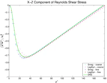
◦, Smagorinsky on fine grid;_∗, Lagrangian dynamic on fine grid. . . 25 3.2 A comparison of the x-z component of the Reynolds shear stress tensor

using different turbulence models at different grid resolutions. ¤, Smagorinsky on coarse grid (64 _× 64 _× 96); +, Lagrangian dynamic on coarse grid; _◦, Smagorinsky on fine grid (128 _× 96 _× 128); _∗, Lagrangian dynamic on fine grid. . . 26

× ×

◦, Smagorinsky on fine grid (128_× 96_×128); _∗, Lagrangian dynamic on fine grid. . . 27 3.4 The rms values of spanwise velocity fluctuations: ¤, Smagorinsky on

coarse grid (64 _× 64_× 96); +, Lagrangian dynamic on coarse grid;_◦, Smagorinsky on fine grid (128_×96_×128);_∗, Lagrangian dynamic on fine grid. . . 28 3.5 The rms values of wall-normal velocity fluctuations: ¤, Smagorinsky

on coarse grid (64_×64_× 96); +, Lagrangian dynamic on coarse grid;

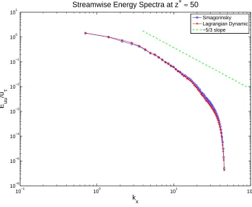
◦, Smagorinsky on fine grid (128_× 96_×128); _∗, Lagrangian dynamic on fine grid. . . 29 3.6 Streamwise spectra of turbulent kinetic energy normalized with friction

velocity at approximately z+

≈50 for Reτ = 180 on fine resolution mesh (128 _× 96_× 128). . . 30 3.7 The mean streamwise velocity of turbulent channel flow at Reτ = 395

compared to DNS results [59]. Only the Lagrangian dynamic model was used. . . 31 3.8 The x-z component of Reynolds stress from Reτ = 395 turbulent

chan-nel flow compared to DNS results [59]. Only the Lagrangian dynamic model was used. . . 32 3.9 A visualization of vortical flow structures using the Q-criterion for the

Reτ = 395 turbulent channel flow. The mesh size used was 192_×128_×384.33

the boundary. Solid nodes are assigned values by using interpolation reconstruction schemes involving the image nodes that implicitly ap-plies the boundary condition. . . 36 4.2 A sketch of the cut-cell method. Cells intersecting the solid are

re-shaped, creating an unstructured mesh at the solid-fluid interface. Cut-ting the cell essentially reshapes the control volume that the governing equations are solved over. . . 37 4.3 A sketch of the indirect imposition approach. A line normal to the

surface (triangle) is projected through the immersed boundary node (green circle) until it intersects a plane of resolved values (orange squares). The resolved values are interpolated onto the line and then another interpolation is performed along the line to impose the bound-ary condition at the immersed boundbound-ary node. . . 38 4.4 Sketch of the reconstruction scheme at an IB point, where a line is

projected along the normal direction of the nearest triangular element into the fluid domain. . . 43 4.5 Streamlines of flow over a circular cylinder at Re = 20. . . 46 4.6 Streamlines of flow over a circular cylinder at Re = 40. . . 46 4.7 Theucomponent of centerline velocity in the wake behind the circular

cylinder for both Re = 20 and Re = 40 in a domain of 31D_×24D. Results are compared to Nieuwstadt and Keller [61]. . . 47

512_×192_×64 and the separation between wall and first u-component was 30 wall units. IBM reconstruction schemes: _∗, logarithmic; _◦, linear 54 5.2 The surface created by the STL geometry of Bolund Hill used in this

paper. The wind flow direction is parallel to the superimposed line with the windward side being the escarpment. . . 57 5.3 Closeup of a Cartesian mesh slice in the x-z plane superimposed on the

Bolund Hill STL. One cell has dimensions of 4 m in the x and 1 m in the z. . . 57 5.4 Wind speedup 5 m above ground along the 270◦_{line. The experimental}

data is found in Berg et al. [6]. . . 58 5.5 Instantaneous wind velocity along the 270◦ _{line. The existence of}

turbulent flow structures and vortex shedding in the wake demonstrate that the LES is able to generate eddies well but requires better bound-ary layer shear stresses to compute wind speed correctly. . . 58 5.6 Ensemble-averaged wind velocity along the 270◦ _{line. The acceleration}

at the escarpment and the evidence of a wake are encouraging results. . 59 5.7 Instantaneous wind velocity vectors approximately 7 m from base of

hill indicating the present flow solver does capture some of the effects of the complex terrain. . . 59 5.8 Comparison of normalized mean wind velocity along the 270◦ _{line (∗),}

2 m south of the 270◦_{line (◦) and 2 m north of the 270}◦_{line (¤) reveals}

that the results are quite sensitive to the location meaning Bolund Hill is not an ideal case for simulation evaluation. . . 61

GPU – Graphics Processing Unit

CFD – Computational Fluid Dynamics

ABL – Atmospheric Boundary Layer

CUDA – Compute Unified Device Architecture

MPI – Message Passing Interface

LES– Large-eddy Simulation

SGS – Subgrid Scale

IBM – Immersed Boundary Method

NWP – Numerical Weather Prediction

ARMA – Autoregressive Moving Average

CHAPTER 1

INTRODUCTION

The integration of more renewable energy resources into our electrical power grids is driven by several factors including: energy security and stability; environmental and climate changes concerns; and economics. Wind energy has the potential to become a larger energy resource in the United States, however producing electricity from wind is far more complicated than just installing more wind turbines. Grid integration is a major challenge, the focus being how to balance the load on the grid given the highly variable nature of the wind. Economics is always a concern with the cost of additional transmission lines, wind turbine manufacturing, and the maintenance of wind farms. The uncertainty of forecasting wind power generation for short periods of time (anywhere from an hour to a few days) is a challenge as well, since the results from existing short-term wind forecasting capabilities vary greatly depending on the location and time period investigated [10, 60, 82]. These and other challenges are further described in a Department of Energy (DOE) report, 20% Wind by 2030 [93].

Overprediction of wind power generation forces utility companies to curtail power generation causing monetary losses for the wind fleet [11, 81]. In general, uncertainty in wind speed and wind power generation causes economic losses for both utility companies and the wind fleet. Reducing the uncertainty would be beneficial to both parties.

Improvements in wind forecasting is the subject of several research projects in recent years [10, 60, 82]. Numerical weather prediction (NWP) models solve the complex mathematical models for wind velocity, temperature, pressure, and moisture using mesoscale initial conditions provided by weather services to estimate the wind conditions at wind farm locations [82]. The mesoscale is on the order of 1 km to 100 km horizontal spatial resolutions. The microscale, the scale applicable to wind turbines, is less than 2 km [77]. The challenge is then to reduce uncertainty in transforming mesoscale information to the microscale.

suffers from the same disadvantages. Even though improvements have been made over the years, no approach can be considered universally applicable to all wind farm locations and a significant uncertainty still exists that would be beneficial to reduce.

1.1

Thesis Statement

The focus of this thesis is to provide a foundation for a short-term wind forecasting capability that involves modeling the atmospheric boundary layer (ABL) over complex terrain at the microscale. A comprehensive microscale wind forecasting model has to consider atmospheric stability while taking into account the effect of surface roughness and fluxes of heat and moisture. Therefore, turbulence modeling and imposing complex terrain boundary conditions are of the utmost importance. For the core components, large-eddy simulation (LES) will be hybridized with Reynolds-averaged Navier-Stokes (RANS) for turbulence modeling. The immersed boundary method (IBM) is then adopted to impose the complex terrain boundary conditions.

resources and turn around times, particularly at high Reynolds numbers [70]. RANS does not need as much resolution as LES and is more widely adopted for industrial applications.

For wind forecasting and other atmospheric studies, LES is desirable for the detail it provides with highly separated flows but today’s computational resources today do not allow for fully-resolved LES at high Reynolds numbers. Also, SGS models in LES do not take into account surface roughness or fluxes of heat and moisture at the surface. Using RANS greatly reduces the amount of computational grid points needed in the near-wall region and can act as a sort of wall model for the LES [75]. RANS can also provide a shear stress near the surface. Correct specification of stresses at the surface is critical because any misprediction can lead to erroneous results in the domain. Surface roughness and fluxes of heat and moisture can also be taken into account with RANS turbulence models [4]. One technique that is practical to implement is to hybridize the RANS and LES techniques where RANS acts as a sort of wall model for LES. However, the differences in the scales of LES and RANS causes a challenge when hybridizing the two approaches but several methods have been investigated [70]. Since micro-scale ABL flows are highly turbulent, a hybrid RANS/LES approach will be implemented similar to Senocak et al. [78].

to complex terrain. Therefore, this thesis will extend an IBM described in Gilmanov et al. [25] that uses a stereolithography (STL) file of an arbitrarily complex object to micro-scale ABL flows over complex terrain using techniques proposed by Senocak et al. [79].

After implementing the hybrid RANS/LES and IBM, the wind simulation will be tested on Bolund Hill. Bolund is a small, isolated hill located off the coast of Denmark. It is 12 m high and is almost completely surrounded by water. Recently, Bolund Hill has been the subject of several numerical and experimental studies, and it constitutes a good test case to evaluate the accuracy and performance of wind models.

The forecasting time horizon for this particular simulation is short-term and requires use of high-performance supercomputing technologies. In recent years, the graphics processing unit (GPU) has become the new paradigm in high performance parallel computing for the tremendous speedups it provides to most numerical simula-tions, and the cost-efficiency of these performance gains. GPUs are used in a variety of fields including computational fluid dynamics (CFD), medical imaging, and molecular dynamics [65, 66], to name a few.

GPUs provide the potential of greatly reducing the turn around time of climate and meteorological models, which could greatly improve the speed of the weather forecasting capability that we have today. GPU computing can also provide the necessary performance gains to broaden the adoption of more intensive flow solver techniques and weather forecasting methods, such as ensemble forecasting [27, 45], which are considered infeasible due to long turn around times and significant compu-tational resources. Therefore, the flow solver techniques are programmed for clusters with NVIDIA GPU accelerators.

incompress-ible, three-dimensional flow solver that is the prior work of Julien Thibault [85] and Thibault and Senocak [86], who developed a GPU-accelerated laminar flow solver that was demonstrated as a basis for an urban dispersion model, and Dana Jacobsen [34], who transformed the work of Thibault for use on GPU clusters [36, 37] and created a full-depth parallel geometric multigrid solver with an amalgamation strategy for the pressure Poisson equation [35]. Also, the pre-processor for the IBM (described later in Section 4.2) was jointly developed by the author of this thesis along with Kyle Felzien, a student in Computer Science at Boise State University [17].

1.2

Works Published

Works published as part of this thesis:

• R. DeLeon, I. Senocak, “GPU-accelerated Large-Eddy Simulation of Turbu-lent Channel Flows,” 50th AIAA Aerospace Sciences Meeting, Nashville, TN, January 2012.

• R. DeLeon, D. Jacobsen, I. Senocak, “Large Eddy Simulations of Turbulent Incompressible Flows on GPU Clusters,” pre-print, Computing in Science and Engineering, March 2012.

• R. DeLeon, K. Felzien, I. Senocak, “Immersed Boundary Turbulent Flow Sim-ulations on GPU Clusters,” Poster presented at the NVIDIA GPU Technology Conference, San Jose, CA, May 2012.

CHAPTER 2

TECHNICAL BACKGROUND

This chapter provides the governing equations and numerical methods used in this flow solver. The core components for the wind solver are accelerated by the massively-parallel, many-core graphics processing unit (GPU) to realize a forecasting capability. A discussion of the GPU and the programming implementation of the previous GPU-accelerated, incompressible flow solver [34, 85] that is the starting point for the wind forecasting capability developed in this study is also included.

2.1

Governing Equations

The governing equations for LES of incompressible flows are the filtered form of the Navier-Stokes equations given as,

∂uj

∂xj

= 0 (2.1)

∂ui

∂t + ∂ ∂xj

(uiuj) =− 1 ρ ∂p ∂xi + ∂ ∂xj ¡

2νSij −τij

¢

, (2.2)

where

Sij = 1 2

µ

∂ui

∂xj

+∂uj

∂xi

¶

is the deformation tensor, and

τij =uiuj−uiuj (2.4)

is the tensor representing the interaction of the subgrid-scales on the resolved large-scales. The overbar in these equations represents a filtered quantity. The numerical mesh typically provides this filter.

2.2

Numerical Methods

The governing equations were solved on a directionally-uniform Cartesian grid using the projection algorithm [15] with second-order central difference schemes for spatial derivatives and a second-order Adams-Bashforth scheme for time advance-ment. The projection algorithm predicts the velocity by removing the pressure term from the governing Navier-Stokes equations to get

u∗ _=ut_{+ ∆t}¡

−ut_{∇ ·}ut+ν_∇2

ut¢. (2.5)

A Poisson equation for pressure can then be written by imposing a divergence free condition on the velocity field at time t+ 1,

∇2

Pt+1

= ρ ∆t∇ ·u

∗_{. (2.6)}

ut+1

=u∗ ₋∆t

ρ ∇P

t+1

. (2.7)

The basic idea behind multigrid [12, 88] is to solve the problem on multiple meshes to reduce long- and short-wavelength errors and accelerate the convergence. The most basic multigrid routine, termed the V-cycle, is to coarsen the original mesh in levels (i.e., repeatedly halving the number of grid points) until the coarsest mesh possible is achieved. Coarsening the mesh is referred to as restriction. The solution is solved at each level to smooth the results until the coarsest mesh is achieved. The solution is directly solved on the coarsest grid and then interpolated back up the levels to the original mesh in the prolongation stage.

2.3

GPU Computing

previously had been two different pipelines, one for pixel shaders and the other for vertex shaders. With one pipeline, a programmer could easily harness all the resources on a GPU [42, 76]. Along with a GPU whose architecture was tailored towards scientific computations, NVIDIA also released the CUDA C programming language [63]. CUDA C, commonly referred to as just CUDA, is a very scalable, single instruction on multiple data (SIMD) language that is an extension of C. Because scientists no longer had to learn complicated graphics languages, the GPU was rapidly adopted by the scientific computing community for the massive data parallelism that could be achieved by the GPU hardware.

GPUs can provide significant speedups to traditional CPU codes. However, one must know the architecture of the GPU and the optimal programming techniques to realize these speedups [62]. While adding a bit more rigor to the programming task, disregarding the architecture may cause an application to run slower than its CPU counterpart. For a forecasting application where speed is essential, optimizing the code to best exploit the GPU architecture is also essential.

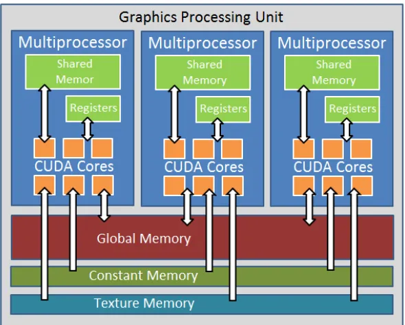
Figure 2.1: A simple illustration of a CUDA-enabled GPU hardware architecture. Ac-tual configurations of streaming multiprocessors and CUDA cores vary depending on the particular model of NVIDIA GPU. The two-headed arrows show how information is transferred between different components.

specific SM [42]. NVIDIA GPUs have onboard dedicated memory referred to as global memory that can be used by any SM but is slower to access than the shared memory or thread registers [62]. The global memory is used to transfer data between the device (GPU) and the host (CPU) memory. Some GPUs, such as the NVIDIA Tesla C2075, have up to 6 GB of onboard memory and 448 SPs allowing researchers to tackle very large problems.

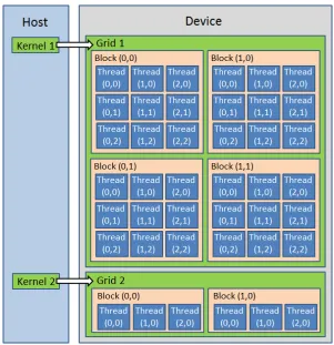
Figure 2.2: A simple depiction of the CUDA programming model. The kernel is initiated on the CPU and then divided up into a grid of blocks. Each block, which consists of multiple threads, is then given to a SM. Note that different grid sizes can be used for different kernels.

Figure 2.2 illustrates how blocks and threads are arranged.

and the thread accesses should reflect this same alignment otherwise performance decreases. Aligned thread accesses are not always possible and therefore global memory accesses must be coalesced [63]. Minimizing the amount of host-device data transfer is also imperative for achieving maximum performance due to the very slow bandwidth of CPU/GPU communication compared to the bandwidth of global memory accesses [62].

2.4

GPU Cluster Implementation

The work performed for this thesis was built upon a flow solver first developed by Julien Thibault [85] and later advanced by Dana Jacobsen [34]. Their work and others [35–37, 86] created a parallel three-dimensional, incompressible Navier-Stokes flow solver accelerated by multiple GPUs that uses dual-level parallelism by interleaving CUDA and Message Passing Interface (MPI). The same programming optimizations in the previous flow solver are adopted in the algorithms used in the current study.

MPI [30] is a parallel programming language that consists of portable message-passing systems that allows multiple processes to communicate with each other. Similar to CUDA, MPI is a C-based language. In the present flow solver, MPI handles the coarse-grain parallelism (partitioning the data into large sections) while CUDA handles the fine-grain parallelism (executing parallel instructions on individual data elements).

copy-ing operations uscopy-ing CUDA streams. Non-blockcopy-ing communication routines allow the program to continue without having to finish the data transfer. Asynchronous memory transfer are also non-blocking and allow the program to continue without the completion of the CPU/GPU data transfer. This communication strategy is described in detail in Jacobsen’s thesis [34] and in Jacobsen et al. [37].

CHAPTER 3

LARGE-EDDY SIMULATION TECHNIQUE

LES uses the idea that larger eddies, which interact with and extract energy from the mean flow, are highly dependent on the geometry of the problem domain, boundary conditions and body forces, while smaller eddies exhibit a more universal behavior being nearly isotropic [94]. Therefore, the effect of the smaller eddies could be captured by a model while the larger eddies could be resolved. Mathematically, this can be accomplished by specifying a cutoff length with a mathematical low-pass filter. The smaller eddies that pass below the filter are called subgrid-scale (SGS) eddies and must be replaced by a SGS model [48]. Several challenges face LES. One comes from the replacement of SGS eddies with a model that introduces errors to the simulation [75]. Another is the computational expense of wall-bounded flows at high Reynolds numbers [94]. A third challenge is boundary conditions introducing errors when the flow is not deterministically known, particularly with inflow conditions that do not introduce the proper turbulent kinetic energy and flow structure information [39].

showed the feasibility of three-dimensional computation of turbulence. This led to future studies [58, 72, 74] of LES applied to turbulent channel flow to gain a better understanding of wall-bounded turbulent flows. Throughout the years, development of several SGS models and tremendous advances in computational hardware have enabled LES to make a major impact in applications such as combustion, aero-dynamics of vehicles, aero-acoustics, propulsion, turbomachinery, and atmospheric modeling [48, 75].

LES is one of three numerical approaches to turbulence calculation. The other two are Reynolds-averaged Navier-Stokes (RANS) and direct numerical simulation (DNS). In the RANS approach, the governing equations are time-averaged such that the resulting quantities are mean values. This is the least computationally expensive form of turbulence calculation and is thus widely adopted in industry [94]. However, RANS cannot resolve most flow structures given the time-averaged governing equations and requires an additional turbulence model to account for their effect. To date, no single turbulence model can be considered universal for turbulent flow simulations, and therefore must be chosen depending on the flow scenario. The DNS approach numerically resolves all scales of turbulent flow as is by far the most computationally expensive. For example, a modest Reynolds number of 104

would require approximately 109

grid points in a DNS [94]. Thus, DNS is primarily used in fundamental turbulence research.

will be the focus of future work.

The full resolution of boundary layers at high Reynolds numbers using LES is im-practical. Thus, wall models have been proposed to alleviate the near-wall resolution requirements by modeling the inner-layer scales with a velocity profile relating the outer-layer velocity to wall stress or using a Reynolds-averaged parametrization. Pi-omelli [70] gives a survey of wall-modeling methods for LES with some examples being the use of a constant-stress shear layer near the wall or using a hybrid RANS/LES methods that uses RANS to calculate the near-wall flow while LES calculates the flow away from the wall. In the present study, a hybrid RANS/LES approach is implemented.

3.1

Subgrid Scale Models

backscatter of energy but does not dissipate energy well and is typically blended with an eddy-viscosity model [53]. The present study uses the Lagrangian dynamic model [54] based on the original Smagorinsky eddy-viscosity model for its applicability to complex geometries and practicality of implementation.

The original Smagorinsky model [80] is perhaps the most popular SGS model but has well-known deficiencies. The model parameters are constant and are chosen a priori [16]. Constant parameters do not cause the eddy viscosity to vanish at near wall boundaries. An ad hoc fix to the problem is to use van Driest damping [18].

In 1991, Germano et al. [21] proposed an alternative method to dynamically calculate the empirical parameters in a SGS model using information from the re-solved velocity field. The dynamic Smagorinsky model introduced by Germano et al. correctly predicts a decaying eddy viscosity near wall boundaries, but it has the disadvantage of requiring homogeneous directions in the flow problem at hand, which has later been addressed by other researchers [22, 54, 71].

The original Smagorinsky model relates local SGS stresses with the local rate of strain on the large-scale eddies. It is given by

τij =−2νtSij + 1

3τiiδij (3.1)

where νt is the turbulent or SGS eddy viscosity and is calculated by

νt= (CS∆)2

q

2SijSij. (3.2)

∆ is the filter width and can be defined by either a mathematical filter (e.g., top-hat filter) or by using the numerical grid as ∆ = √3

proper CS value, which depends upon the mesh and the flow problem being inves-tigated, is critical. For wall boundaries in a channel flow, the model parameter CS must be adjusted to reflect the vanishing eddies by multiplyingCS with the van-Driest damping function [18], which is given as

1₋exp

µ

−y+

A

¶

, (3.3)

wherey+

is the non-dimensional distance given in wall units andAis a constant that is approximately 25.

Damping the Smagorinsky coefficient through an arbitrary function significantly improves the LES results, but the procedure is ad-hoc and does not readily extend to complex geometry. This particular shortcoming is overcome by the adopting the dynamic procedure [21, 49, 69]. The dynamic procedure uses information from the existing flow field to calculate the model coefficient dynamically while the simulation is advancing.

The first dynamic subgrid scale model was proposed by Germano et al. [21]. In their dynamic procedure, a second filter with a larger width, denoted by the hat, is applied to a resolved field. The basis of the dynamic procedure is the Germano identity

Lij =Tij −cτij. (3.4)

The individual terms in this algebraic relation are given by

Tij =udiuj −ubiubj, (3.5)

c

The tensor,Lij, is referred to as the Leonard stresses and can be calculated as follows

Lij =udiuj −ubiubi. (3.7)

Using the Germano identity and the Smagorinsky model, Germano et al. [21] proposed to calculate CS by

C2

S = 1 2

­

LijSij

® ­

MijSij

®, (3.8)

which uses spatial averaging in homogeneous directions as denoted by the angle brackets. The advantages of this method are that an arbitrary damping function is no longer required to make eddy viscosity diminish near walls and determination of ana priori CS is no longer necessary. The dynamic Smagorinsky model was later modified by Lilly [49] who used a least-squares method to obtain

C2

S = 1 2

hLijMiji hMijMiji

. (3.9)

In both cases, the tensor, Mij, is given by

Mij = 2∆2

h

\

|S_|Sij−α2|Sb|bSij

i

, (3.10)

There-fore, Meneveau et al. [54] proposed a dynamic model from a Lagrangian perspective by averaging along the flow pathlines rather than in homogeneous directions. The idea is to minimize the error caused by using the Smagorinsky model and the Germano identity by taking previous information along the pathline to obtain a current value. This formulation applies to fully inhomogeneous turbulent flows as seen in many en-gineering applications and requires less computational resources than other localized dynamic models [22], therefore making it a practical option in fluids engineering.

The Lagrangian dynamic model uses backward time integration and an expo-nential weighting function that decreases the weight of past events. The weighted backward time integration can then be written as two relaxation-transport equations

∂_JLM

∂t +u· ∇JLM =

1

T (LijMij− JLM), (3.11) ∂_JM M

∂t +u· ∇JM M =

1

T (MijMij − JM M), (3.12)

where T is the relaxation time scale. Meneveau et al. [54] chose to define T as

T = 1.5∆ (_{JLMJM M})−1/8

. (3.13)

After solving Equations 3.11 and 3.12, the value of CS is then calculated using the relation,

C2

S = J LM JM M

, (3.14)

which can be directly substituted into the Smagorinsky eddy-viscosity model.

model requires two filters. The base filter is the computational mesh. A simple top-hat filter is used as the second filter in the Lagrangian dynamic model. Time advancement in the Lagrangian dynamic model (Equations 3.11 and 3.12) is performed using the first-order schemes recommended by Meneveau et al. [54], which are given as

Jn+1

LM (x) =H

©

ǫ[LijMij]n

+1

(x) + (1₋ǫ)_JLMn (x₋un∆t)ª, (3.15) Jn+1

M M(x) = ǫ[MijMij]n

+1

(x) + (1₋ǫ)_{JM M}n (x₋un∆t), (3.16)

where

ǫ= ∆t/T n

1 + ∆t/Tn (3.17)

and T is defined in Equation 3.13. The ramp function in Equation 3.15 is required to clip away negative C2

3.2

Validation of the LES Technique

Periodic turbulent channel flow at Reτ = 180 and 395 were used to validate the LES capability. The dimensions of the computational domain are (2πδ, πδ,2δ) in (x, y, z) where δ is the channel half-height, x, y and z are the streamwise, spanwise, and wall-normal directions, respectively. Two grids were used for the Reτ = 180 case, a coarse resolution mesh with 64 _× 64 _× 96 points, and a fine resolution mesh with 128 _× 96 _× 128 points. Grid stretching was not applied in the wall-normal direction because a structured adaptive mesh refinement strategy is envisioned in future extensions of the present wind solver.

The turbulent channel flow was initialized in an approach similar to Gowardhan [28] that superimposes a sinusoidal fluctuating component on a logarithmic profile as in

u=uτ

µ

1

κlny

+

+ 5.5

¶

+ sin (πz) cosxsiny, (3.18)

v =₋(1 + cos (πz) ) sinxsiny, (3.19)

w=₋πsin (πz) sinxcosy. (3.20)

The fluctuating components can be scaled by a constant. However, because periodic boundary conditions are imposed in the streamwise directions, the amplitude of the fluctuations did not matter for the current cases as the solution eventually converges on to a statistically stationary turbulent state. Thus, the sinusoidal fluctuation amplitudes were set to unity.

Figure 3.1: A comparison of the mean streamwise velocity profiles using different models and mesh sizes (coarse - 64_×64_×96, fine - 128_×96_×128): ¤, Smagorinsky on coarse grid; +, Lagrangian dynamic on coarse grid; _◦, Smagorinsky on fine grid;

∗, Lagrangian dynamic on fine grid.

Periodic boundary conditions [29] were applied in the stream- and span-wise directions to both velocity and scalar quantities. On channel walls, the no-slip condition was imposed on the velocity field, and Neumann boundary conditions for pressure and the scalar quantities found in the Lagrangian dynamic model were set to zero. The flow was maintained by imposing a height independent constant pressure gradient in the streamwise direction that is u2

τ/δ. The simulation was allowed to develop for 200 dimensionless time units (uτt/δ). Statistics were sampled for 20 dimensionless time units.

Figure 3.2: A comparison of the x-z component of the Reynolds shear stress tensor using different turbulence models at different grid resolutions. ¤, Smagorinsky on coarse grid (64 _× 64 _× 96); +, Lagrangian dynamic on coarse grid; _◦, Smagorinsky on fine grid (128 _×96 _× 128); _∗, Lagrangian dynamic on fine grid.

Smagorinsky model with van Driest damping and the Lagrangian dynamic model. The profiles were compared to both the theoretical law of the wall and the DNS performed by Moser et al. [59]. As expected, the finer mesh did considerably better than the coarse mesh, having two points in the viscous sublayer as opposed to one.

All simulations did well with the x-z component of the Reynolds shear stress as depicted in Figure 3.2. The Smagorinsky model gave a higher Reynolds shear stress near the wall than the DNS while the Lagrangian dynamic model gave lower values than the DNS. Both models gave larger values of Reynolds shear stress away from the wall, particularly the Lagrangian dynamic at the coarse grid resolution.

Figure 3.4: The rms values of spanwise velocity fluctuations: ¤, Smagorinsky on coarse grid (64 _× 64 _× 96); +, Lagrangian dynamic on coarse grid; _◦, Smagorinsky on fine grid (128 _×96 _× 128); _∗, Lagrangian dynamic on fine grid.

3.3-3.5. With the streamwise velocity fluctuations in Figure 3.3, the coarse grid Lagrangian dynamic model does worse than the coarse grid Smagorinsky toward the center of the channel but better toward the wall. However, the fine grid approaches yields the exact opposite, with the Smagorinsky model performing better toward the wall but worse away from the wall. With the velocity fluctuations in the spanwise direction (Figure 3.4) and the wall-normal direction (Figure 3.5), the Smagorinsky model gives better results than the Lagrangian dynamic model, on both grids.

10−1 100 101 102 10−6

10−5 10−4 10−3 10−2 10−1 100 101

k x

E uu

/u τ

Streamwise Energy Spectra at z+≈ 50

Smagorinsky Lagrangian Dynamic −5/3 slope

Figure 3.6: Streamwise spectra of turbulent kinetic energy normalized with friction velocity at approximately z+

≈50 for Reτ = 180 on fine resolution mesh (128 _× 96 × 128).

slope close to theoretical one roughly around wavenumbers five through ten.

Figure 3.8: The x-z component of Reynolds stress from Reτ = 395 turbulent channel flow compared to DNS results [59]. Only the Lagrangian dynamic model was used.

turbulent flow [48]. The abundance of flow structures depicted in Figure 3.9 is an outcome of LES where large-scale motions are resolved in the computations.

Figure 3.9: A visualization of vortical flow structures using the Q-criterion for the Reτ = 395 turbulent channel flow. The mesh size used was 192_×128_×384.

CHAPTER 4

IMMERSED BOUNDARY METHOD

Immersed boundary method (IBM) is a numerical technique that imposes bound-ary conditions created by embedded solids on Cartesian meshes. This technique eliminates the cumbersome task of generating body-fitted grids. Body-fitted grids may not be suitable for a short-term wind forecasting over highly complex terrain because of the possibility of skewed cells that would introduce significant error to the solution. Also, Cartesian meshes fit much more naturally to the GPU architecture as opposed to unstructured body-fitted grids, resulting in better acceleration of the computations. For these reasons, IBM was chosen for this study. This chapter provides general details of IBM and the specific details of the implementation.

4.1

Overview of Immersed Boundary Methods

accuracy of the body force terms and the stability of computations has been the focus of many studies.

There are two primary approaches in IBM: continuous forcing and discrete forcing. The discrete forcing approach is used in the present study. The continuous forcing approach came about when the IBM concept was first proposed by Peskin [67] to simulate blood flow in a heart using a Cartesian mesh. This approach adds a body forcing term to the governing equationsbefore discretization, requiring the numerical method to resolve another continuous term. The continuous forcing approach works well for flow involving elastic boundaries, which usually falls into biological [9, 68] and multiphase flows [89, 92]. The disadvantage of the continuous forcing approach is formulating a proper body force term without creating additional numerical stability constraints in flow with rigid bodies [56].

The discrete forcing method, proposed by Mohd-Yusof [57] and later applied by Verzicco et al. [95], remedied the numerical stability issue by imposing the forcing term

after the governing equations are discretized, eliminating the need for calculating an additional continuous term in the governing equations. The discrete forcing method can be categorized further into two different groups of boundary condition imposition: indirect and direct. Indirect imposition is used in this thesis.

Figure 4.2: A sketch of the cut-cell method. Cells intersecting the solid are reshaped, creating an unstructured mesh at the solid-fluid interface. Cutting the cell essentially reshapes the control volume that the governing equations are solved over.

implicitly applies the boundary condition. As an example, linear interpolation of the velocity at the boundary between a solid node and its corresponding image node should be zero after reconstruction.

The cut-cell method [91] is another direct imposition approach used in finite volume methods. This creates an unstructured grid around the solid by reshaping cells intersecting the solid, as shown in Figure 4.2. Cutting the cell essentially reshapes the control volume that the governing equations are solved over. This approach guarantees the conservation of mass and momentum since control volumes are adjusted to conform with the solid when using a finite volume approach.

the components required for the indirect imposition approach. A line normal to the surface is projected such that it passes through the immersed boundary node that will eventually intersect a plane of resolved fluid nodes. The resolved values are interpolated onto the line and then another interpolation is performed along the line to impose the boundary condition at the immersed boundary node. This indirect approach has been successfully applied by Fadlun et al. [19], Verzicco et al. [95], and Iaccarino and Verzicco [32] for engineering fluid flow applications at moderate Reynolds numbers.

The treatment of the pressure boundary condition at the immersed boundary is different among authors. Fadlun et al. [19] explain that because of the linearization of the governing equations at the immersed boundary, the pressure gradient in the normal direction is zero and an explicit application of a Neumann boundary condition is not necessary. They also described how not including the Neumann pressure bound-ary condition varies the solution on the order of 10−3

-10−4

for a linear reconstruction. This was also implemented in Balaras [1]. Kim et al. [41] describe a mass source/sink term in the pressure Poisson equation defined as (in two dimensions)

q=₋u1 ∆x −

v1

∆y =

1

∆x∆y(−uˆ1∆y−vˆ1∆x) (4.1)

whereu1 andv1 are the vector components inside the solid and the hat on the velocity

that provides consistency between pressure and velocity. The present study follows Fadlun et al. [19] with no explicit application of the Neumann pressure boundary condition.

4.2

Velocity Reconstruction Scheme

The discrete forcing with indirect boundary imposition was chosen for this flow solver because Cartesian meshes are well-suited for the GPU architecture and RANS will provide a mean velocity profile near the surface so a direct boundary imposition isn’t necessary. In the discrete forcing IBM, a solid boundary is represented by adding a forcing term to the momentum equations given in Equation 2.2. The discretized form of the u-momentum equation is

un+1

i −uni

∆t =RHSi+Fi, (4.2)

whereRHSi includes the pressure gradient, convective, and diffusive terms, as well as SGS terms when addressing turbulent flows. Using the direct forcing method [19, 57], the velocity at the boundary can be prescribed asun+1

i =Vn

+1

i , then the body force becomes

Fi =−RHSi+

Vn+1

i −uni

∆t , (4.3)

on grid points near the solid geometry. The steps in applying the IB method within the projection algorithm are summarized as follows

1. In the preprocessing stage, separate the Cartesian cells as solid, fluid, or im-mersed boundary (IB). Determine the necessary parameters for the velocity field reconstruction schemes.

2. Predict the velocity by solving the momentum equations as per the projection algorithm.

3. Set the solid Cartesian cells to zero and apply reconstruction scheme to IB nodes.

4. Solve the pressure Poisson equation by imposing the divergence free condition.

5. Correct the velocity field and set solid cells to zero.

For this application, the reconstruction scheme used will be similar to the IBM approach described in Gilmanov et al. [23–25] but will be extended to atmospheric flows with a rough surface following the approach described in [79]. No Neumann pressure boundary condition is applied in the IBM because studies by Fadlun et al. [19] have shown the error of omitting this step is very small (on the order of 103

−104

).

of the CAD geometry with the underlying Cartesian mesh. The preprocessor was jointly created by Kyle Felzien, a computer science undergraduate student at Boise State University, the author of this thesis, and Senocak [17].

The first stage of the preprocessor identifies all Cartesian points within the small search radius, ds0, from the solid boundary. The value of the search radius is

determined by finding the maximum distance from opposite corners of a cell (i.e.

ds0 =

p

dx2_+dy2_+dz2_{). The position vectors of these points, rN B, are compared}

to the position vector of the mth triangular element’s centroid, rm+1/2, until the

following condition is satisfied

min

m=1,M|rN B−rm+1/2|< ds0. (4.4)

Any point that satisfies the above condition is called a near-boundary node. Note that near-boundary nodes can be either internal or external to the solid boundary.

The next stage is to determine which of the near-boundary points are actually within the solid. For every near-boundary point, all triangular elements located within the search radius centered at the near-boundary node are identified. Examining the sign of the scalar product,nm+1/2·(rnb−rm+1/2), determines whether a near-boundary

point is internal or external to the solid boundary. Ifnm+1/2·(rnb−rm+1/2)>0 forat least onetriangular element within the sphere from the point, then the Cartesian mesh point is external to the body and flagged as an IB node. Ifnm+1/2·(rnb−rm+1/2)<0

Figure 4.4: Sketch of the reconstruction scheme at an IB point, where a line is projected along the normal direction of the nearest triangular element into the fluid domain.

4.3

Extending the Reconstruction Scheme to Atmospheric

Boundary Layer Flows

The linear interpolation reconstruction scheme may also work well for turbulent flows if the grid resolution is fine enough to capture the viscous sublayer where

u+

= y+

as suggested by the law of the wall. However, a clear viscous sublayer does not exist within the ABL due to the rough surface. A linear interpolation scheme could underestimate the surface stresses, because a logarithmic or power wind profile is typically observed in atmospheric flows. One also has to consider how the reconstruction scheme influences the SGS model. A consistency between the underlying assumptions in the turbulence model and the IBM reconstruction scheme is desirable to obtain satisfactory results. Therefore, a logarithmic reconstruction scheme [79] is proposed so when combined with Prandtl’s mixing length model [94] (discussed later), the aforementioned consistency is maintained.

Atmospheric flows over complex terrain are influenced by roughness, atmospheric stability, and fluxes of sensible and latent heat and moisture, all of which play a major role in the observed wind profiles. Typically, the boundary conditions are imposed through stress and flux terms

τ =ρu′_w′ _(4.5)

H =ρCpw′Θ′ (4.6)

E =ρw′_q′ _(4.7)

where τ is the turbulent stress at the surface, H and E are the fluxes for heat and moisture, respectively. u′_{, w}′_{, Θ}′_{, q}′ _{represents the fluctuations of streamwise wind,}

implementa-tion of these terms in Equaimplementa-tions 4.5-4.7 within an immersed boundary method would be tedious and can complicate the IBM, which has historically become popular due to the simplicity of its implementation. Therefore, the reconstruction schemes should operate only on the primitive variables (e.g.,u,v,w, Θ,q) to retain the simplicity of the IB method for atmospheric flows computations.

The reconstruction scheme proposed is the log-law reconstruction scheme [79] because of its consistency with the Monin-Obukhov similarity theory for neutral sta-bility conditions that is also used in turbulence model assumptions. The logarithmic reconstruction is derived from the assumption that friction velocity remains constant in the direction normal to the wall. Therefore, similarity in the velocity profile is maintained at different distances from the wall. Dividing the rough surface log-law,

U uτ = 1 κln µ z z0 ¶ , (4.8)

where z0 is the equivalent roughness height at the boundary results in

U1 =U2

·

ln (z1/z0)

ln (z2/z0)

¸

, (4.9)

where U1 and U2 are the magnitude of the velocity at locations shown in Figure 4.4,

and z1 and z2 are the normal distances to the surface along the IB line as shown in

Figure 4.4. The magnitude of the velocity must then be broken down into u, v and

Figure 4.5: Streamlines of flow over a circular cylinder at Re = 20.

Figure 4.6: Streamlines of flow over a circular cylinder at Re = 40.

4.4

Immersed Boundary Method Validation

Laminar flow over a circular cylinder at Reynolds numbers of 20 and 40 were used to validate the immersed boundary implementation. The domain was 31D_×24D

in the x and z directions, respectively, where x is the direction of flow and D is the diameter of the cylinder. The center of the cylinder was placed at 10.5D in the x

direction and at the halfway point in the z direction. The boundary conditions were an inlet and convective outlet in the streamwise direction with all other boundary condition set to freeslip. A linear reconstruction scheme was applied to this flow scenario. The resolution of the mesh was 1024 _×768 with 64 cells in the longitudinal direction. Approximately 30 cells were placed with the diameter of the cylinder.

The streamlines are presented in Figures 4.5 and 4.6. Figure 4.7 shows the u

Figure 4.7: The u component of centerline velocity in the wake behind the circular cylinder for both Re = 20 and Re = 40 in a domain of 31D_× 24D. Results are compared to Nieuwstadt and Keller [61].

CHAPTER 5

WIND FLOW OVER COMPLEX TERRAIN

In this chapter, the methods described in preceding chapters are extended to sim-ulate wind flow over complex terrain. A literature review on recent wind forecasting techniques is also provided. The IBM extended to atmospheric flows as described in Section 4.3 along with a hybrid RAN/LES method will be implemented since fully resolving the ABL with LES is impractical. Results of wind flow over a complex terrain are presented as well.

5.1

Brief Survey of Wind Forecasting Over Complex Terrain

Medium-term forecasts generally range from 6 hours to a day while long-Medium-term forecasts are measured in days.

In the present survey, only short-term wind forecasting techniques are reviewed. The most basic short-term wind forecasting model that often serves as a benchmark for new models is a persistence model [27]. A persistence model uses the assumption that the future value will equal the current value [81]. Persistence models typically work well within an hour or two but the quality of the results rapidly degrades when the time horizon is increased.

There are two additional wind forecasting approaches that typically produce better results than persistence models: the physical approach and the statistical approach [82]. The physical approach is based on using numerical weather prediction (NWP) models. NWP solves the complex mathematical models describing wind flow over complex terrain, temperature, and pressure. A major challenge of this approach is the uncertainty when using the mesoscale wind speeds provided by a weather service on the microscale spatial domain of the wind farm site [45]. NWP requires significant computational resources and are often limited to medium- and long-term forecasts because of the difficulty of providing the mesoscale weather information. The best results are obtained in neutrally stratified weather conditions [82].

ensemble forecasting is to take a combination of different NWP implementations with the same initial conditions to produce a frequency distribution, but it still requires the same resources as ensemble forecasting [45].

The statistical approach to wind forecasting is the use of time series using the auto-regressive moving average (ARMA). The basic idea of ARMA is to estimate a future value of an individual time series as a linear combination of previously observed values [27]. There are several derivatives to the ARMA approach [10, 60, 82] including the Box-Jenkins approach of autoregressive integrated moving average (ARIMA), the seasonally adjusted ARIMA (SARIMA), and the approach of fractional-ARIMA (f-ARIMA), to name a few. There are several other time series techniques that have been employed and surveys of these are given in Bhaskar et al. [10] and Soman et al. [82].

A popular area of wind forecasting research in recent years has been in artificial neural networks (ANN) [10]. The ANN technique is based on artificial intelligence where the program mimics the human learning process to discover relationships between the variables in a system [31]. ANN does not require explicit declarations of mathematical expressions and thus takes less development and computational time than ARMA models [10]. Depending on the implementation and application, ANN models can produce better or worse results than ARMA models as shown by comparing the conclusions of Gomes and Castro [27] and Soman et al. [82].

A physical approach is pursued in this study. Statistical approaches provide good results for short time horizons but the accuracy of the results degrade as the time horizon is extended. Typically, physical approaches are useful for medium-and long-term forecasts (> 6 hours) because of the amount of computations and difficulty obtaining information in short time horizons [82]. Hence, the simulation has been developed for GPU clusters for their potential to accelerate the computations to predict in the short-term while still maintaining the applicability to longer time horizons. Also, time series only provide mean wind velocity predictions. Resolving the wind in the ABL can provide predictions on the mean and random components of wind velocity as well as other quantities such as pressure and temperature.

5.2

IBM in Atmospheric Flows

IBM in meteorological applications is not without precedent. Senocak et al. [79] extended the discrete forcing approach to atmospheric boundary layer simulations over a flat terrain by adopting the same length scale assumptions in the turbulence model and reconstruction schemes. Lundquist et al. [52] presented a 2D implementa-tion of the ghost-cell approach within the Weather Research and Forecasting Model (WRF) for analytical geometries without any consideration for turbulence modeling and turbulent stresses at the immersed surfaces. Jafari et al. [38] performed a RANS simulation of wind flow over complex terrain also using a ghost-cell approach.

turbulence modeling and lay the foundation for future incorporation of models that maintain atmospheric stability and account for land-surface fluxes. One of the first steps is to couple the IBM with a logarithmic reconstruction schemes described in Chapter 4 with a hybrid RANS/LES turbulence modeling technique.

5.3

Hybrid RANS/LES

The LES technique is pursued because of the information it provides on turbulent fluctuations and has potential to capture the details of highly separated flows that are found in wind flow over complex terrain. The Lagrangian dynamic Smagorinsky model was chosen for the SGS model because homogeneous directions of turbulence are not a requirement. However, LES requires resolution in the viscous sublayer and with Reynolds numbers being on the order of 107

along with the surface being rough, fully resolving the boundary layer is impractical. This is the motivation for hybridizing LES with RANS at high Reynolds numbers to form a hybrid RANS/LES technique. RANS models the contribution of the near-wall eddies and acts as a sort of wall model for the LES. Hybrid RANS/LES has been applied to atmospheric scenarios with success in Senocak et al. [78], Bechmann et al. [5] and Bechmann and Sørensen [4], to name a few. There are several methods to hybridize LES and RANS [75], but the method chosen for this simulation is the smooth length scale transition suggested by Senocak et al. [78]

νt=

"µ

1₋exp

µ

−z h

¶¶2

(CS∆)

2 + exp µ −z h ¶2

(κz)2

#

|S_|, (5.1)

main-tains consistency with the mixing length turbulence model. The transition height is determined by the following relationship based on the Nyquist theorem,

γ = h

2∆, (5.2)

where ∆ is the base filter width and γ is a parameter chosen depending on the flow. The value ofγ dictates how many cells near the wall are modeled by RANS. Ensuring thath is large enough to encompass at least one full cell is of the utmost importance, particularly when the aspect ratio of a cell is larger in the wall-normal direction than in the lateral directions.

5.4

Evaluation of Hybrid RANS/LES

The consistent coupling of the hybrid RANS/LES and IBM implementations were evaluated using periodic turbulent channel flow (see Chapter 3). The friction Reynolds number was set to 1000 to ensure a sufficiently large log-law region. The dimensions of the channel were also increased to (8πδ,3πδ,2δ) in (x, y, z). To test the IBM, the walls were placed such that they were not coincident with any of the grid points, but were still parallel to the x-y plane. Thirty wall units separated a wall to the firstucomponent. The computational grid was chosen to be 512_× 192_×64. No grid stretching was applied. Note the z dimension is actually larger than the height of the channel to maintain the thirty wall unit separation. The same forcing, initial conditions and time sampling intervals used in the LES validation were applied. A length scale transition height for the hybrid RANS/LES was chosen to be 4∆ or γ

100 101 102 103 0

5 10 15 20 25

z+

u

+

Linear Reconstruction Logarithmic Reconstruction Log Law

Viscous Sublayer

Figure 5.1 is a comparison of different IBM reconstruction schemes to the the-oretical law of the wall. A logarithmic reconstruction scheme (Equation 4.9) was developed using smooth wall log-law given as,

U uτ

= 1

κln

³_yuτ

ν

´

+B, (5.3)

where κ is the von K´arm´an constant and B is a constant. The value of the von K´arm´an constant is 0.41 and B is 5.2 [73]. The logarithmic reconstruction performs much better than the linear reconstruction. The linear reconstruction severely under-predicts the velocity. On the other hand, the logarithmic reconstruction provides more reasonable result consistent with the law of the wall. The underprediction of velocity with linear reconstruction is not surprising, since the separation between the wall and the first calculated component is 30 wall units. At this distance, linear relations present in the viscous sublayer no longer hold and forcing a linear relationship does not provide the proper shear stress near the wall. The distance is in the region where the log-law holds, and therefore logarithmic reconstruction agrees well with theory.

5.5

Bolund Hill Performance Tests

Using the implementation described in Sections 5.2 and 5.3, simulations were performed on Bolund Hill, a 12-meter-high isolated coastal hill located in Roskilde Fjord, Denmark. Because of its isolation and small shape, it has been the subject of several studies, both experimental [6] and computational [3, 38].

Figure 5.2 is a surface rendering of the Bolund Hill stereolithography (STL) file used in this paper. The feature that makes the Bolund Hill case challenging to simulate is the steep vertical escarpment. Figure 5.3 shows a slice of the Cartesian mesh used superimposed on the STL at the escarpment. In this solver, the x and y

directions correspond to the lateral directions andz to the vertical direction, with the

x direction being perpendicular to the escarpment in Figure 5.2. The computational Cartesian mesh used in this paper was 256 _×192 _×128 in the x,y, andz directions, respectively, with a lateral resolution of 4 m and vertical resolution of 1 m. A no-slip condition was imposed at the terrain surface with a free-slip condition at the top of the domain and periodic lateral boundary conditions. The equivalent roughness height for the logarithmic reconstruction (Equation 4.9) was 0.0003 m for the water and 0.015 m for the hill as was suggested in Berg et al. [6]. A height-independent, constant forcing of 0.001 was applied.

In the Bolund Hill Experiment, masts with sonic anemometers were set up along in the vicinity of the line in Figure 5.2. This line is referred to as the 270◦ _{line in the}

Bolund Experiment when the escarpment is the windward side. The simulation was compared to data of wind 5 m above the ground along the 270◦ _{line. Figure 5.4 shows}

the velocity sampled over the hill normalized to a value sampled from the reference mast [3, 6]. The results are not very satisfactory and deviate from the experimental data but several factors may be responsible for the erroneous results.

Figure 5.2: The surface created by the STL geometry of Bolund Hill used in this paper. The wind flow direction is parallel to the superimposed line with the windward side being the escarpment.

−100 −50 0 50 100 150 0.4

0.6 0.8 1 1.2 1.4 1.6 1.8 2

Relative Position (m)

Normalized Wind Speed, U/U

ref

Figure 5.4: Wind speedup 5 m above ground along the 270◦ _{line. The experimental}

data is found in Berg et al. [6].

Figure 5.5: Instantaneous wind velocity along the 270◦ _{line. The existence of}

Figure 5.6: Ensemble-averaged wind velocity along the 270◦ _{line. The acceleration at}

the escarpment and the evidence of a wake are encouraging results.

and may incorrectly influence the upstream velocity. While the influence might be minor because of the hill having a low profile, replacing the periodic lateral boundary conditions with open lateral boundary conditions would be worthwhile to pursue. Another factor is the spatial resolution, particularly in the vicinity of the surface. As shown in Figure 5.3, only 4 to 6 cells are currently resolving the vertical escarpment. When looking back to the laminar cylinder case, approximately 30 cells were needed to obtain good results. Therefore, grid refinement is necessary. Also, issues with the hybrid RANS/LES and IBM when applied to complex geometry may not have arisen when simple benchmark cases were performed. Further evaluation of these techniques is required. However, Figure 5.4 shows that the acceleration and deceleration of the wind is captured, but the errors in the magnitudes can be attributed errors in the surface stresses.

While unsatisfactory results were obtained in the wind speeds at several locations, the flow solver is able to capture the influence of the complex terrain qualitatively. Figure 5.5 is a visualization of the instantaneous velocity along the 270◦ _{line. The}

existence of turbulent flow structures and vortex shedding demonstrate that the turbulence modeling performs well but requires better boundary layer shear stresses to accurately model atmospheric turbulence.

Figure 5.6 depicts the time-averaged wind velocity values along the 270◦ _line.

The acceleration at the escarpment looks good from a qualitative perspective when compared to results from Jafari et al. [38]. The wake behind the hill compares reasonably well also compared to Jafari et al., again from a qualitative standpoint.

−100 −50 0 50 100 150 0.4 0.6 0.8 1 1.2 1.4 1.6 1.8 2

Relative Position (m)

Normalized Wind Speed, U/U

ref

2 m south 270° line 2 m north

Figure 5.8: Comparison of normalized mean wind velocity along the 270◦ _{line (∗),}

2 m south of the 270◦ _{line (◦) and 2 m north of the 270}◦ _{line (¤) reveals that the}

results are quite sensitive to the location meaning Bolund Hill is not an ideal case for simulation evaluation.

Figure 5.7, although this may be sudden acceleration due to turbulence. This may be an issue that did not arise when testing was performed on simple benchmark cases and prompts further evaluation of the IBM and hybrid RANS/LES.

Figure 5.8 provides another reason for further evaluation of the simulation. This figure compares numerical results along the 270◦ _{line against results from 2 m north}

and south of the same line. The results do not deviate greatly 2 m north of the 270◦

line. However, sampling 2 m south greatly deviates from the other two demonstrating that the results are highly sensitive to the location, which implies that simulation is also highly sensitive to the complex geometry of this particular case. The sensitivity suggests that Bolund Hill is too difficult a complex terrain to be an ideal case for evaluating a simulation. Other simpler test cases should be used alongside this one to gain a better understanding of the model.

× 192 _× 128 case performed at 20% of real-time. That is, for every 5 seconds of computational wall time, 1 second physical time was resolved. The computing platform used consisted of four NVIDIA Tesla C2070 GPUs connected by PCI Express 2.0_×16 buses and a quad data rate (QDR) Infiniband interconnect. Mesh sizes of 192 ×128_×64 and 128_×128_×33 with the same spatial resolutions were also attempted although the results are not shown in this thesis. The 192_×128_×64 mesh performed at approximately 70% of real-time on the same computing platform but with only two GPUs. Using four GPUs resulted in approximately the same performance but a large majority of the GPU remained idle for this problem size.