Identification of hydrodynamic forces developed by flapping fins in a watercraft propulsion flow field

(1)

University of New Orleans University of New Orleans

ScholarWorks@UNO

University of New Orleans Theses and

Dissertations Dissertations and Theses

Fall 12-18-2014

Identification of hydrodynamic forces developed by flapping fins

in a watercraft propulsion flow field

Erdem Aktosun

University of New Orleans, [email protected]

Follow this and additional works at: https://scholarworks.uno.edu/td

Part of the Aerodynamics and Fluid Mechanics Commons, Controls and Control Theory Commons,

Navigation, Guidance, Control and Dynamics Commons, Propulsion and Power Commons, Signal

Processing Commons, and the Systems Engineering and Multidisciplinary Design Optimization Commons

Recommended Citation Recommended Citation

Aktosun, Erdem, "Identification of hydrodynamic forces developed by flapping fins in a watercraft propulsion flow field" (2014). University of New Orleans Theses and Dissertations. 1900.

https://scholarworks.uno.edu/td/1900

This Thesis-Restricted is protected by copyright and/or related rights. It has been brought to you by

ScholarWorks@UNO with permission from the rights-holder(s). You are free to use this Thesis-Restricted in any way that is permitted by the copyright and related rights legislation that applies to your use. For other uses you need to obtain permission from the rights-holder(s) directly, unless additional rights are indicated by a Creative Commons license in the record and/or on the work itself.

(2)

Identification of hydrodynamic forces developed by flapping fins in a watercraft propulsion flow field

A Thesis

Submitted to the Graduate Faculty of the University of New Orleans in partial fulfillment of the requirements for the degree of

Master of Science in

Engineering

By

Erdem Aktosun

B.ScYildiz Technical University, 2010

(3)

Acknowledgments

First of all, I would like to acknowledge Dr. Nikolas Xiros for always having the patience

and knowledge to help guide me to complete this thesis on time.

I would also like to acknowledge the following people for their role in helping me

conquer my feat of this thesis:

 Dr. Kostas A. Belibassakis from National Technical University of Athens for helping me

with getting CFD flapping fins data.

 PHD student Vasileios Tsarsitalidis from National Technical University of Athens for

helping and explaining concept and previous work about flapping fins.

 PHD student Mustafa Arda from Trakya University with helping for MATLAB coding

concept.

 My family and friends for always supporting me through my academic and life

(4)

Table of Contents

List of Figures ... v

List of Tables ... vii

Abstract ... viii

CHAPTER 1 ... 1

Introduction ... 1

1.1 General Overview ... 1

1.2 Purpose of the Study ... 5

CHAPTER 2 ... 7

Review of Literature... 7

2.1 Previous Studies ... 7

2.2 The Investigation of Aerohydrobionts ... 9

2.3 The investigation of the flapping fin theory ... 13

2.4 Kinematics of biomimetic fin thrusters ... 16

2.5 Dynamics of biomimetic fin thrusters ... 17

2.6 Free Surface Effects ... 19

2.7 The outline of CFD code by NTUA ... 20

2.8 Harvesting power and energy by flapping fins ... 23

CHAPTER 3 ... 26

Methodology ... 26

3.1 Data Analysis for Heave Force ... 27

3.2 Describing Function for Heave Force ... 40

3.3 Data Analysis for Surge Force ... 43

CHAPTER 4 ... 62

Results ... 62

4.1 Comparison Transfer Function Model and CFD Data for Heave Force ... 63

4.2 Data points of Surge force ... 74

CHAPTER 5 ... 82

Conclusions ... 82

(5)

5.2 Future Work ... 83

Bibliography ... 84

Appendix ... 88

Appendix A: CFD folder tree made spectrum analysis ... 88

Appendix B: One of the CFD output data ... 89

Appendix C: MATLAB codes ... 91

Appendix D: Spectrum plots for fish15AR4 and fish15AR6 ... 131

Appendix E: Comparison plots for fish15AR4 and fish15AR6 ... 163

(6)

List of Figures

Figure 1: MIT laboratory robot "Robotuna" [1] ... 1

Figure 2: Considered laws of unsteady motion: A: combined translational-rotational oscillations, B: purely translational oscillations, C: purely rotational oscillations, and D: advancing wave-type deformations [1] ... 3

Figure 3: Vortex structures, forming behind the fin, performing heaving oscillations: A: near free surface, B:Near solid flat ground and C: In unbounded fluid [1] ... 4

Figure 4: Cutter on underwater flapping fins [1] ... 14

Figure 5: Russian ship with a fin wave energy extraction system [1] ... 15

Figure 6: Japanese ship with a fin wave energy extraction system [1] ... 15

Figure 7: Description of motion of the flapping fin during CFD experiment [46] ... 16

Figure 8: Flapping fins simulation model in CFD environment ... 18

Figure 9: (a) Ship hull equipped with a horizontal flapping wing located below the keel, forward the ship section. (b) Same hull with a vertical flapping wing located below the keel, at mid-ship [49] ... 21

Figure 10: Schematics of a flow energy harvesting system based upon a flapping fin [50] ... 24

Figure 11: Analog signal [51] ... 27

Figure 12: Discrete – time signal - low sampling rate [51] ... 28

Figure 13: Discrete-time signal - high sampling rate [51] ... 28

Figure 14: Discretization of the time signal [51] ... 30

Figure 15: Dividing of the signal into the two new signals [51] ... 31

Figure 16: Rectangular Fin outline for s/c = 2, 4, 6 respectively [46] ... 33

Figure 17: Fish-like fin outline for s/c=4 and s = 150, 300, 450 respectively [46] ... 34

Figure 18: Cross section area for NACA 0012 [52] ... 34

Figure 19: FFT flow chart ... 36

Figure 20: Heave force spectrum - frequency domain pattern for one type of data ... 37

Figure 26: Describing function heave force system ... 40

Figure 27: Surge force spectrum - frequency domain pattern for one type of data ... 44

(7)

Figure 34: FFT analysis spectrum - frequency for first data series ... 48

Figure 35: Nonlinear surge force system ... 50

Figure 36: Comparison between CFD data and heave force transfer function model ... 68

Figure 42: Magnitudes of H(F,F) ... 74

Figure 43: Phases of H(F,F) ... 75

Figure 44: Magnitudes of H(-F,-F) ... 76

Figure 45: Phases of H(-F,-F) ... 77

Figure 46: Magnitudes of H(-F,F) ... 78

Figure 47: Phases of H(-F,F) ... 79

Figure 48: Magnitudes of H(F,-F) ... 80

(8)

List of Tables

Table 1: Aerohydrodynamic characteristics of various systems [1] ... 10

Table 2: Speed characteristic of some biological and technical systems [23] ... 11

Table 3: fish15AR4, Heave Amplitude = 1m ... 63

Table 4: fish15AR4, Heave Amplitude = 1.5 m ... 64

Table 5: fish15AR4, Heave Amplitude = 2 m ... 64

Table 7: fish15AR6, Heave Amplitude = 1.5 m ... 65

Table 9: Optimization result fish15AR4, Heave Amplitude = 1m ... 66

Table 10: Optimization result fish15AR4, Heave Amplitude = 1.5 m ... 66

Table 11: Optimization result fish15AR4, Heave Amplitude = 2 m ... 66

Table 12: Optimization result fish15AR6, Heave Amplitude = 1 m ... 67

Table 13: Optimization result fish15AR6, Heave Amplitude = 1.5 m ... 67

(9)

Abstract

In this work, the data analysis of oscillating flapping fins is conducted for mathematical

model. Data points of heave and surge force obtained by the CFD (Computational Fluid

Dynamics) for different geometrical kinds of flapping fins. The fin undergoes a combination of

vertical and angular oscillatory motion, while travelling at constant forward speed. The surge

thrust and heave lift are generated by the combined motion of the flapping fins, especially due to

the carrier vehicle’s heave and pitch motion will be investigated to acquire system identification

with CFD data available while the fin pitching motion is selected as a function of fin vertical

motion and it is imposed by an external mechanism. The data series applied to model unsteady

lifting flow around the system will be employed to develop an optimization algorithm to

establish an approximation transfer function model for heave force and obtain a predicting black

box system with nonlinear theory for surge force with fin motion control synthesis.

Flapping fins, flapping fin thruster, biomimetic ship propulsion, energy from waves,

(10)

CHAPTER 1

Introduction

1.1 General Overview

The idea of biomimetic flapping fins based on observations of fish and cetaceans

(swimming marine mammals, e.g whale). The present work of biomimetic fins has given much

information about kinematics. For example, it shows us how these animals use their flapping

tails and fins to produce propulsive and maneuvering forces. In order to understand how these

creatures generate forces, the fin theory needs to be combined with modern fluid mechanics. The

fish tails have high aspect ratio similarly to fins as shown Fig.1. To sum up, these fins have been

investigated by developing kinematics and dynamics model and by calculating its hydrodynamic

response.

Figure 1: MIT laboratory robot "Robotuna" [1]

In general, a basic difference between a biomimetic thruster and a conventional propeller

(11)

pitching (fin) motion, while for the propeller there is only rotational power feeding. In realistic

sea conditions, the ship undergoes a moderate or higher-amplitude oscillatory motion due to

waves, and the vertical ship motion could be exploited for providing one of the modes of

combined/complex oscillatory motion of a biomimetic propulsion system. At the same time, due

to waves, wind and other reasons, ship propulsion energy demand in rough sea is usually

increased well above the corresponding value in calm water for the same speed, especially in the

case of bow/quartering seas.

Many experimental and theoretical analyses have been performed for flapping fins and

fins. The result of these recent research and development efforts illustrates that the flapping fins

systems at optimum conditions can manage high thrust levels [2,3,4]. Furthermore, the

requirements for environment and inter-governmental regulations are getting stricter for ocean

vehicles. According to Kyoto Treaty, the reduction of pollution and environmental impact of

especially ocean vehicles is the great key to effect of global warming and climate change. For

example, the environmental pollution caused by cargo ships all over the world has been

considered as one of the great factors [5,6] contributing to adverse impact on environment due to

bad fuel use of vessels. Another proof about environmental problems is coming from satellite’s

data [7]. It suggests that the main maritime-waterborne of the transportation has permanently

spots with high concentration of pollutants induced by the engine of vessels.

As aforementioned, the study of generation of thrust by flapping fins has been increased

significantly in recent years due to quest for clean energy generation by regulations. The

principles of flapping fins performance analysis is based on fluid mechanics especially

(12)

approximated as fish-like motion which is combination of harmonic heave and pitch motion as

shown in Fig.2.

Figure 2: Considered laws of unsteady motion: A: combined translational-rotational oscillations, B: purely translational oscillations, C: purely rotational oscillations, and D: advancing wave-type deformations [1]

The idea is that fish have their own thrust mechanism and they propel themselves in

water very efficiently due to rhythmic motion of their tail [8]. Propulsion is generated by means

of the combined motion of the tail. Thrust is manageable due to the fact that the combined

(13)

Figure 3: Vortex structures, forming behind the fin, performing heaving oscillations: A: near free surface, B:Near solid flat ground and C: In unbounded fluid [1]

Flapping fins of a thin plate is approached as fish tails in steady forward motion. They are

thought of oscillating with combinations of harmonic heave and pitch motion during calculation

of their thrust performance. However, the hydrodynamics of oscillating fins or thin plates has

been mostly studied in experimental way because there is difficulty of analyzing vortex shedding

induced by boundary layer separation and estimation of nonlinear dynamics of the large vortices

generated by free layers as shown in Fig.3 [8].

Some may raise the question why many scientists have been interested in this field so far.

The answer is the useful advantages of flapping fin system [1] below;

 Can be considered as environmentally friendly

 Relatively low-frequency systems

(14)

 Multi-functional being capable of operating in different regimes of motion

 Can provide static thrust

 Possess more acceptable cavitation characteristics than conventional propellers

 Can provide high maneuverability

1.2 Purpose of the Study

In this study, the data analysis of flapping fin oscillation which is combination of

harmonic heave and pitch motion is implemented for post-processing data from CFD code in

order to perform system identification for heave and surge force. The data results from CFD

include 6 degrees of freedom outputs which are forces and moments. These forces are surge,

sway and heave forces and the moments are roll, pitch and yaw moments. In this work,

especially heave and surge force will be analyzed to develop system identification between

inputs which is the combined motions of flapping fin due to the forward motion of ship in waves

and outputs which are heave and surge force. Note that surge force is playing very important role

to acquire thrust from flapping fin and heave force is very important to get lift action. First of all,

CFD software is very slow to make analysis. If one parameter is changed for calculation, time

needs to be dedicated. In addition, CFD results are not a closed form relationship. Therefore, the

relationship between force and frequency, velocity or amplitude is unknown. As known, force is

a function of the frequency motion, the forward velocity of the vehicle and the amplitude of

motion of the flapping fins. For instance, once one parameter is changed, the effect of change of

this parameter is unknown on force due to unknown relationship. Furthermore, this parameter

could be optimized for better operations. To sum up, the objective of this thesis is to define a

(15)

control system theory and can be used to provide a prediction of relationships based on inputs

(16)

CHAPTER 2

Review of Literature

This chapter includes a review of literature describing previous studies performed and the

fundamental information of flapping fins.

2.1 Previous Studies

The first study was implemented by Leonardo da Vinci to explain and apply the

mechanism of thrust generation by a flapping fin in 1490. Based on studies of Leonardo da

Vinci, at the end of the 19th century and the beginning of the 20th century, many studies were

emerged in this field to develop flight vehicles using flapping fins [9,10]. That time studies about

bionics were limited due to having inadequate scientific and engineering background.

The first explanation of the physics of flapping fins is given by Knoller and Betz [1] in 1909 and

1912 respectively. Both of them reached the conclusion that longitudinal thrust force and vertical

lift force is induced by flapping fin oscillations. However, an extensive research was done about

flapping fin by the end of the 19th century [1]. The first experimental study was implemented by

Katzmayr [11] to verify Knoller – Betz’s work in 1922.

Prandtl studied development of unsteady motion of a fin in incompressible flow and he

concluded that vortices are shed from a sharp trailing edge [1] in 1922. Birnbaum contributed a

linearized solution for Prandtl’s formulation and provided the resultant thrust force generated by

a flapping fin [1]. Also further studies of this unsteady airfoil theory were conducted by Wagner,

Kussner and Glauert. Keldysh and Lavrentiev provided a formulation for thrust generated by a

harmonically oscillating flat plate. The solution was obtained with conformal mapping method

(17)

Golubev developed a flapping fin theory, different from Prandtl’s model, based on the

‘‘discrete’’ Karman form of the wake arrangement. Using the momentum theorem, he obtained

an integral equation whose solution allowed him to obtain the aerodynamic characteristics,

including the thrust of the flapping fin in the 1940s [1].

Polonsky and Bratt analyzed flow visualization experiments to verify von Karman and

Burgers’ observations. They illustrated the existence of different types of vortex structures

behind the oscillating airfoil [1].

Since 1960s, the investigations in this field have been intensified. Many researchers have

been conducting investigations about the aero-hydrodynamics of flapping fins especially

development of more extensive mathematical model [1].

The first symposium regarding bionics was held in Dayton, Ohio in 1960 [12]. Since that

(18)

2.2 The Investigation of Aerohydrobionts

Indeed, the first explanation about thrust generation by flapping fins is released in 1912

[1]. After that, the first study of analysis has been done in and after 1924 [13,14]. During 1960s,

bionics had been emerged in science as a separate field which covers studies of the basics of

flapping-fin propulsion [15]. Many publications in biology and biomechanics aimed to develop

air or water vehicles with flapping fins as well. The major purpose was the explanation of the

background of the efficient propulsion of fish, cetacean, birds, and insects. To sum up, after

understanding of the phenomenon of fish efficient propulsion, the desire of those studies is to

implement and apply that background to air or ocean vehicles with the principles of

hydromechanics mathematical model.

As mentioned earlier, many researchers were interested in flapping fin propulsors coming

from early observation of fish, insects and cetaceans who all utilize oscillating fin mechanisms

for thrust generation. It is useful to introduce the coefficient K which represents

aero-hydro-dynamic mechanisms;

0 0

mU NL

K 

Where; N is the power of the system, m is the mass of system, U0 is the swimming or

flying speed, L0 is the maximum length of the object. The table below shows K coefficient for

(19)

Table 1: Aerohydrodynamic characteristics of various systems [1]

Biological or technical

system

Coefficient of aerohyrodynamic perfection

K (kWs/ton)

Relative speed

U0/L0 (s-1)

Swimming in nature

Cateceans 4.40 0.3-1.0

High-speed fish 3.16 1.0-8.0

Dolphins 0.18 2.0-8.0

“Swimming” in technology

Submersibles 22.0 0.06-0.2

Flying in nature

Birds and insects 15.8 60.0-170.0

“Flying” in technology

Jet airplanes 81.0 4.0-9.0

As can be seen from the table, dolphins have the best hydrodynamic perfection in

comparison with the other systems. However, birds and insects have the highest relative speeds.

Many studies appeared about properties of insect flight, fish and cetaceans in 1920s. The

research was about the structure of the fins, flight modes, kinematics and deformations of the

fins, measurements of different characteristics, and simulations of the flight of insects [1].

Maxworthy [16], Ellington [17,18], Freymuth [19], Liu [20,21] made research about

aerodynamics of insect flight. They realized that unsteady flow properties are very important for

(20)

Another study conducted by Schmidt-Nielsen [22] showing that it is more economical for

an animal to fly rather than to move on land. Table 2 illustrates the comparison between relative

speeds of motion for living creatures and man-made objects [23].

Table 2: Speed characteristic of some biological and technical systems [23]

Biological or technical system Maximum speed (body lengths/s)

Human being 4

Cheetah 18

Supersonic aircraft 75

Starling (a type of bird) 120

Pershin [24] and Kozlov [25] have studied about fish and cetaceans to look into the

propulsive characteristics of these creatures. They systematized and analyzed bio-hydrodynamic

of properties of swimming. According to many studies about bio-hydrodynamics, there is a

correlation between the method of thrust generation, speed of displacement and typical regimes

of swimming for the creature. According to observations, low-speed marine creatures utilize

wave-type propulsors, like a whole part of body contributing for thrust generation. Therefore,

body flexibility is proportional to speed, i.e as increasing speed causes rise in flexibility of body.

High-speed sea creatures can be considered by a “system” that has three main functional

parts: a hull, a stem, and a fin. In follows, that “stem-fin” subsystem has 2 degrees of freedom.

The displacement of fin can be considered as heaving-pitching oscillations [1].

According to Pershin [24] and Kozlov [25], the analysis of statistical data of hydrobionts

(21)

parameters. The most important parameters are the dimensional speed, frequency, and amplitude

of oscillation.

Many papers addressed kinematics of hydrobionts [24,26,27,28]. They showed that the

body, stem and fin have a relation with the swimming velocity and average period of oscillation.

Furthermore, the type of motion made by marine creature such as dolphins has been investigated

in literature. According to some papers, the motion of hydrobionts is sinusoidal type. However,

analysis of swimming motion based on underwater films of Cousteau, has shown that during

uniform translatory motion the oscillatory motion of the stem and the fin is close to a harmonic

motion.

The oscillations of fins are optimized in dolphins to avoid flow separation. Thus,

kinematic parameters of motion which are heave and pitch oscillations having have phase shift

between them. The pitch oscillations are following the heave oscillation by an angle close to ψ =

π/2 [24].

To sum up, the main parameters of hydrobionts that can be as similar to human-made devices

can be [1];

 Dimensions, shape and platform of the fin

 Amplitude of the fin oscillations

 Frequency of oscillations

 Mass-rigidity characteristics of the fin (variable chordwise or spanwise)

(22)

2.3 The investigation of the flapping fin theory

The mathematical model of flapping fin theory is based on linearized inviscid

two-dimensional (2-D) flow. Along with rise of computer technology, more complex 3-D fin

nonlinear inviscid and viscous approaches were introduced.

Keldysh and Lavrentiev implemented the linear theory to obtain thrust force acting on

thin oscillating plate. They used conformal mapping to solve the problem [1]. Furthermore,

Garrick provided a solution about same problem by using Theodorsen’s linearized solution for

incompressible unsteady flow past a flat plate.

Meticulous investigations of flapping fins propulsors were done by Khaskind, Sedov and

Nekrasov to make performance analysis for heaving, pitching and combined oscillations. The

forces acting on the oscillating thin plate were found by solving a singular integral equation [1].

Another analysis of combined heaving-pitching oscillating fin has been done by Gorelov

to look into the maximum thrust force achievement. He reached the conclusion that the

maximum thrust force is managed when there is a phase angle ψ=π/2 between heave and pitch

motions.

Gorelov was the person to develop the propulsive characteristics of a flapping fin in

nonlinear formulation. He obtained a solution by the method of discrete vortices and compared

his result with suction force obtained by linear theory.

Instead of the method of discrete vortices, panel method which is a nonlinear formulation

is used to investigate performance of the propulsive characteristics of flapping fins due to its

(23)

effect of fin thickness, oscillation amplitude, phase shift, pitch axis location, and Strouhal

number [1].

In addition to these studies, many investigations have been conducted about mathematical

modeling of flow past flapping fin systems, two-dimensional flow models, three-dimensional

flow models and experimental investigations of flapping fins. Taking account of all these studies,

the application of flapping fins have been used in ship and offshore industry. Recently, many

projects are being conducted to improve water vehicles which utilize flapping fins.

Indeed, one of the first tests of full-scale vehicles with flapping fin propulsors was

implemented by Grebeshov in 1970s. He conducted the experiment a full-size cutter on hydro

fins. This cutter used hydro fins not only as lifting but also as propulsive components as shown

Fig.4.

Figure 4: Cutter on underwater flapping fins [1]

The major work is recently going on in American, Canadian, British and German

scientific institutes. This work is published by Muller [33]. In addition, we have Russian and

(24)

Figure 5: Russian ship with a fin wave energy extraction system [1]

Figure 6: Japanese ship with a fin wave energy extraction system [1]

Last but not least, other work about flapping fins development can be found in Refs.

[36,37,38,39,40,41,42,43,44,45]. Among these works, some of them are about biomechanics

aspects related to the structure of fins of birds and insects and the mechanics and dynamics of

their flight. The others are suggested aero-hydro-dynamics of flapping fins and to the practical

(25)

2.4 Kinematics of biomimetic fin thrusters

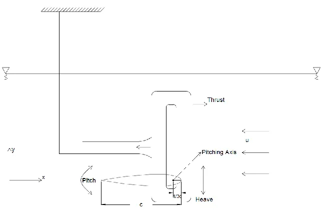
Figure 7: Description of motion of the flapping fin during CFD experiment [46]

In this section, it is indicated that the classical mechanisms which describes the motion of

flapping fins without consideration of the causes of motion applied by NTUA (National

Technical University of Athens) team (Dr. Kostas A. Belibassakis and PHD student Vasileios

Tsarsitalidis). As can be seen in Fig.7, the reference coordinate system is considered for flapping

fins. Therefore, the motion of body with flapping fins can be described in accordance to this

coordinate system such as translational (surge, heave and sway motions) and oscillatory (roll,

pitch and yaw motions). As shown in Fig.7 under constant parallel velocity, the flapping fin

coordinate system is experiencing a combination of both heave motion and pitch motion due to

the waves. In this case, two different basic frequencies have been considered for the motion of

flapping fin, one of them is relative frequency [47];

1 1 2f

 

And the other frequency is flapping fin pitching frequency;

2 2 2f

(26)

In the simple harmonic thrust producing case, relative frequency and flapping fin pitching

frequency is equal to each other [47].

 

1  2  And f1  f2  f

The surge motion of the flapping fin is shown as below

Ut t

x( )

And t indicates time here. The vertical motion becomes;

) 2 sin( )

(t h₀ ft

h  

Where; h0 is amplitude of vertical oscillation of the flapping fin. Simultaneously, the fin

undergoes a pitch oscillatory motion at a possibly different frequency yet as it is mentioned

before in the simple harmonic thrust producing case motions of the frequencies are equal.

Therefore, pitch oscillatory motion becomes [47];

) 2

sin( )

(  0  

 t  m ft

Where θm is mean angle of attack, θ0 is amplitude of pitch oscillation of the flapping fin

and ψ is phase angle between the two movements.

2.5 Dynamics of biomimetic fin thrusters

The phase difference ψ between the two oscillatory motions is very important as far as

the efficiency of the thrust development by the flapping system is concerned. As it is discussed

before in the simple harmonic thrust producing case where: 1 2 , it usually takes value

ψ = 900

. With the pivot point for the angular motion of the fin located around the 1/3 chord

length from the leading edge, a minimization of the required torque for pitching is achieved as

(27)

Figure 8: Flapping fins simulation model in CFD environment

For flapping systems steadily advancing in unbounded liquid the main flow parameter

controlling the unsteady lift production mechanism is the Strouhal number [46];

U fh St2 0 / ,

Note that theReynolds number has a secondary role affecting viscous drag corrections.

As a result of the simultaneous heaving and pitching motions of the biomimetic fin the

instantaneous angle of attack is given by [47]:

) ( ) / (

tan ) ( ) ( )

(t H t  t 1 U 1dh dt  t

      

For relatively low amplitudes of purely harmonic motion and optimum phase difference

(28)

) cos( ) (

)

(t U 1h₀ ₀ t

   

which is equivalently achieved by setting the pitch angle θ(t) proportional to θH(t)

) / (

tan )

(t w 1 U1dh dt



and thus

U wh0 /

0 

 

Where; w is termed the ‘pitch control parameter’ after [47], usually taking values in

0<w<1, which is amenable to optimization. Decreasing the value of w, the maximum angle of

attack is reduced and the fin operates at lighter loads. On the contrary, by increasing the above

parameter the fin loading becomes higher and so is the chance of leading edge separation that

would lead to significant dynamic stall effects. Following [48], we exploit the above relation, as

an active pitch control rule of the flapping-fin thruster in the general polychromatic case, based

on the time history of vertical motion. In this case, the instantaneous angle of attack is [48]

) / ( tan ) 1 ( )

(t  w 1 U1dh dt



2.6 Free Surface Effects

In the case of the biomimetic system under the calm or wavy free surface, additional

parameters enriches the above set, as the Froude number;

(29)

where L denotes the characteristic (ship) length and g is gravitational acceleration, as

well as various frequency parameter(s) associated with the incoming wave, like μ = ω2L/g and τ

= ωU/g, τ has distinguish subcritical (τ <1 / 4) from supercritical (τ >1 / 4) condition [49].

2.7 The outline of CFD code by NTUA

The hydrodynamic analysis of ship and flapping fins are employed by NTUA team (Dr.

Kostas A. Belibassakis and PHD student Vasileios Tsarsitalidis). First, the hydrodynamic

analysis of ship is computed by developing algorithm in computational fluid dynamics

environment. The flapping fin is considered as appendage of a specific ship and by following the

hydrodynamic analysis of the ship, the hydrodynamic analysis of the flapping fin is employed as

well. The combined translational and pitch motion of the flapping fin is induced by the ship (49).

Both vertical and horizontal of arrangement of flapping fin is analyzed in this study (46,48,49) as

shown in Fig.9. The pitching motion of the fin about its pivot axis is selected properly in order to

produce thrust, with significant reduction of reduction of responses and generation of anti-rolling

(30)

Figure 9: (a) Ship hull equipped with a horizontal flapping wing located below the keel, forward the mid-ship section. (b) Same hull with a vertical flapping wing located below the keel, at mid-ship [49]

Ship hydrodynamic analysis has been applied by using linear theory using a Rankine

source-sink formulation and ship motions are calculated considering the additional forces and

moments because of unsteady propulsion systems.

Standard linearized sea-keeping analysis is used to achieve the motions and responses of

ship and flapping fin. The motion equations of ship (the coupled equation of heave and pitch

motion of the ship) can be calculated regarding the mass of ship, added mass and damping

(31)

A simplified lifting line model is applied for hydrodynamic analysis of flapping fin to

obtain expressions of the flapping fin forces (49). The generated flapping forces are considered

as two parts. One part is depending on the oscillatory ship amplitudes and the other part is

dependent on the incoming wave potential. The first part produces modifications of the

hydrodynamic coefficients of the system the other part adds on Froude-Krylov and diffraction

forces in the right hand side (49).

The horizontal arrangement of the flapping fin thruster and vertical flapping fin in

quartering and beam waves can be seen in detail (49). To sum up, the analysis of flapping fins

(32)

2.8 Harvesting power and energy by flapping fins

Besides energy harvesting from application of propellers, flapping fins have a capability

of generating energy as well. We are getting energy from flapping fins induced by vortices,

free-surface waves and uniform currents. In the first case, at least two different methods are

considered to generate energy from the flapping fins; the constructive mode and the destructive

mode. In the constructive mode, the vortices created by the fin and the incoming vortex are in the

same phase and reinforce each other [50]. The destructive mode, on the other hand, is

characterized by a phase difference of approximately 1800 between the fin-generated vortices

and the incoming ones [50].

Related to these studies, generating flapping fin energy from free-surface waves has also

been experienced. According to some studies, submerged fins have the ability to propel itself

forward in sea conditions once it is right under a free surface.

According to some investigations, the coupling of different motion modes and external activation

is required in order to generate energy from flapping fins. For instance, one of modes of flapping

fin is acted as a periodic motion. Hydro-dynamically, this produces periodic variations in the

lifting and drag forces as well as pitching- rolling moments in an incoming flow. These

time-varying forces/moments in their turn can trigger other modes from which power extraction is

(33)

Figure 10: Schematics of a flow energy harvesting system based upon a flapping fin [50]

Two-dimensional fin is integrated with a damper c in incoming flow U as shown in

Fig.10. ρ is the fluid density. Here, chord length is 1m. The fin has a combined motion which is

heave and pitch as described before. Both motions are defined as harmonic motion. Heave

motion has already been described as

) 2 sin( )

(t h₀ ft

h  

And also pitch motion has been defined as below;

) 2 cos( )

(t ₀ ft

 

Inertia of the fin is ignored. The external moment is needed to trigger the pitching mode

as Me = -M. M is defined here as hydrodynamic pitching moment. The power input into the

system becomes;



 _M

M P_i  _e 

The power input is obtained by the damper c and it can be expressed as;

2

(34)

The mean power input becomes;





 _t _T

t i i dt P T P 0 0 1

And the mean power output becomes;





 _t _T

t Podt

T P 0 0 1 0

Where, T is defined period of the system. Finally, net power of the system becomes;

i

o P

P

P 

In addition, the efficiency of system is analyzed with respect to net power of the system.

The power harvesting efficiency becomes

P Y U P 2 ) 2 / 1 (   

Where; YP is calculated as difference between the highest vertical position reached by the

(35)

CHAPTER 3

Methodology

Flapping fins motion was previously describing the combination of heave and pitch

motion in chapter 2. All outputs which are forces and moments have been analyzed in CFD code

based on the input which is the motion of flapping fins. Therefore, we have discussed how to

describe physics behind flapping fin motion. In addition, in order to define system identification,

the correlation between input (motion of fin) and output (heave and surge force) needs to be

implemented. To do this, surge force (fx) and heave force (fy) depending on time needs to be

transformed in frequency domain. Hence, Fourier Transform, as well as the method used to

transform both forces in frequency domain will be discussed in this section. Furthermore, an

optimization method will be developed in MATLAB in order to establish approximating transfer

function model for heave force. Nonlinear model is implemented in order to find data points of

(36)

3.1 Data Analysis for Heave Force

In this section, a brief presentation of Fourier analysis is given. What kind of data do we

get out of this model and why do we choose to work these data series. In addition to this, how do

we validate our Fourier methodology based on our data series?

In general, Fourier series can transform any periodic signal or function into harmonic

signals or sinusoidal functions. Therefore, all periodic functions can be analyzed easier by using

Fourier Transform. There are many reasons to utilize Fast Fourier Transform (FFT). However,

the fundamental idea is using FFT in many science fields to transform time-domain signals into

frequency-domain signals. This approach is very useful to define parameters of vibrating systems

[51].

The use of digital technology is on the rise in various applications because digital signal

processing has many advantages in comparison to analog signal processing. In this study, heave

and surge force data series are based upon discrete time signals. Therefore, FFT (Fast Fourier

Transform) has been applied to all heave force signals to transform into frequency domain by

using MATLAB. Unlike analog type of signals which are essentially continuous time signals,

digital technology encodes information using discrete-time signals as shown Fig.11 and Fig.12

[51].

(37)

Figure 12: Discrete – time signal - low sampling rate [51]

If the variable to be represented requires fast transitions, it must be described by using a

higher sampling rate as shown in Fig.13 [51].

Figure 13: Discrete-time signal - high sampling rate [51]

In this study, the output which is heave and surge force data series is assumed to consist

of periodic functions. Therefore, any initial transient stage is ignored. For period –T≤ t ≤ T surge

force can be described as below.

) 2

sin( )

(t c₀c₂ ft y

Where; y(t) is the function (signal) in time domain and c0 and c2 are coefficients of series.

(38)

With using Euler’s formula and Fourier integral, the transform of output function into

frequency domain becomes;





 



 y t e dt Y() ( ) i2ft

Where ω is angular frequency and Y(ω) is a function of amplitude and phase spectrum of

output. This equation is called Fourier Transform of y(t). This analog Fourier Transform will be

needed to find data points of the system as well in the next section. However, due to the fact that

our data series of heave and surges force are composed of discrete signals (564 data), Fast

Fourier Transform methodology needs to be explained briefly. Based on the FFT algorithm, the

expression of frequency domain of heave and surge forces have been obtained in MATLAB for

each data series. First of all, the methodology of FFT will be explained and then how FFT

algorithm is implemented to surge force will be clarified.

The Fast Fourier Transform (FFT) is a very useful algorithm for Discrete Fourier

Transform (DFT). By using DFT computation time is decreased from N2 to Nlog2N where N is

number of samples of each surge force data series. Discretization of the time signal needed for

(39)

Figure 14: Discretization of the time signal [51]

FFT algorithm is based on the fact that every discrete Fourier transform with N samples

can be divided into two Fourier transforms, each with N/2 samples (first with even samples and

(40)

Figure 15: Dividing of the signal into the two new signals [51]

Fourier Transform becomes sum of two new smaller Fourier transforms:

 



   1 0 2 N r N fr i r

f Ye

Y 



         1 2 0 ) 1 2 ( 2 ) 1 2 ( 1 2 0 ) 2 ( 2 2 N r N r f i r N r N r f i

re Y e

Y  







       1 2 0 1 2 0 2 / 2 ) 1 2 ( 2 2 / 2 2 N r N r N fr i r N f i N fr i

re e Y e

Y

 



Where r is sample number. We have two new Fourier transforms in equations above so

that they can be defined by real variables [51]



   1 2 0 2 / 2 2 N r N fr i r

f Y e

A 



    1 2 0 2 / 2 ) 1 2 ( N r N fr i r

f Y e

B



(41)

N i

e W



2





Because equations can be combined between each other, FFT equation which is used for

most of digital signal processing can be obtained as below [51];

f f f

f A W B

Y  

It is better to explain output data series structure before explaining how Fourier

Transform applied to surge force and heave force data series. For each selection of geometry,

amplitude of vertical oscillation of the flapping fin to chord ratio h/c, phase angle between heave

motions and pitch oscillation ψ, the mean angle of attack θm are created and all files

corresponding to this set are gathered. This typical set has simulations for five Strouhal numbers

ranging from 0.1 to 0.7 and the amplitude of pitch oscillation from 5 degreeto maximum 75

degree. For each run, the mean angle of attack θm is 0 degree and phase angle ψ is 900[46].

As shown in Appendix B, 564 output data series are obtained from CFD. Each column

includes iterations, time, surge force, heave force, sway force, roll moment, yaw moment and

pitch moment respectively [46]. Strouhal number ‘Str’ and pitch motion amplitude θ0 define each

run, ‘its’ stands for the time steps used and time for the simulated duration. All forces and

moments are the mean values divided by water density ρ, pow stands for power (also divided by

ρ), tra stands for translational and rot stands for rotational., numbers 1,2,3 stands for the axes

x,y,z and min, max, dev stand for minimum, maximum and standard deviation values

Regarding geometrical parameter during CFD experiment, NACA 0012 standard fin is

used for all data series. As far as an individual flapping fin is concerned, the selection of

platform area, in conjunction with horizontal/vertical sweep and twist angles, and generating

(42)

the set of the most important geometrical parameters. Other important parameters are the fin

aspect ratio, span-wise distribution of chord, thickness and possibly camber of fin sections, as

well as the specific fin-sectional forms. Here, some of fin geometries regarding rectangular and

fish type used for experiment are presented in Fig.16, Fig.17 and Fig.18;

(43)

Figure 17: Fish-like fin outline for s/c=4 and s = 150, 300, 450 respectively [46]

Figure 18: Cross section area for NACA 0012 [52]

As it was mentioned before two types of fins were used in data structure which is fish

like and rectangular fins. The geometric parameters are aspect ratio (AR) and skewback angle

(such fish15). For each selection of geometry, heave to chord ratio, phase angle, mean angle of

attack and position of pitching axis is created.

As known, 6 degrees of freedom 3 forces and 3 moments induced from the oscillating

fins. In this study, surge force and heave force are chosen to be analyzed. From the aspect of

hydrodynamics and control point of engineering, surge force is playing fundamental role to

(44)

First of all, FFT (Fast Fourier Transform) needs to be calculated and illustrated in some

kind of framework in order to make data analysis for heave force data series. In MATLAB, an

algorithm is developed to transform heave force data into the Fourier domain. Due to the fact

that heave force time signals are discrete type of signal, Fast Fourier Transform, FFT is applied

for all heave force signal in order to compute dominant frequency. The excitation frequency is

needed to be computed in order to decide the system is whether linear or nonlinear and what kind

of transfer function model can be used to make data fitting for all heave force data series. To do

this the formula as below can be used to calculate the excitation frequency which is for heave

and pitch motion.

0

2h StU fm otion 

Where; fmotion becomes excitation frequency for each data, St is Strouhal number, U is

flow velocity and h0 is heave motion amplitude that can be calculated as below;

c h h₀ 

h/c is heave to chord ratio which is defined for each data and c is chord length that is 1m

for all type of fins . Now, for all data FFT analysis results can be seen in Appendix D. The way

(45)

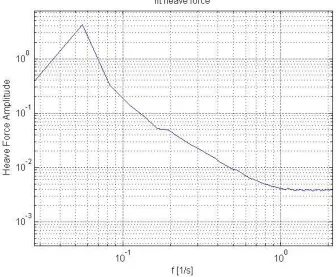
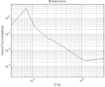
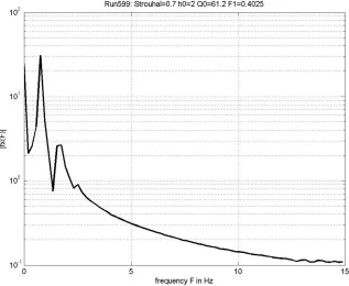
However, some of them that were identified as representative of important cases can be seen in log-log plots for heave force data series in Fig.20, Fig.21, Fig.22, Fig.23, Fig.24 and Fig.25;

(46)

Figure 20: Heave force spectrum - frequency domain pattern for one type of data

(47)

(48)

(49)

All plots generated in MATLAB have been observed to achieve data analysis and define

heave force system after Fast Fourier Transform for all data series. The first order frequency has

been become dominant frequency of all data spectrum which means the peak frequency is equal

to the excitation frequency which is the frequency of motions for almost each data series.

Therefore, heave force system is acting such as linear system. We can collect data points by

calculating the value of spectrum with respect to excitation frequency on the spectrum plots. All

data points have been calculated by developing codes in MATLAB. Now, the heave force system

is ready to develop describing function to build transfer function between inputs and outputs.

3.2 Describing Function for Heave Force

The data fitting concept achieved for heave force data series is explained in this section.

Transfer function will be generated between inputs and outputs for each amplitude to create

mathematical model for this system as shown in Fig.26.

Figure 26: Describing function heave force system

Since CFD data points have been gotten, second order transfer function is used for data

fitting with respect to different fish type geometries and different operational conditions

depending on heave and pitch motion amplitude. For suitable data fitting process, the sample

second order transfer function as below is used to compare to CFD data series for heave force

(50)

) 200 )( 100 ( ) ( ) ( ^     s s z s k s H

The purpose is to find the gain k and zero z along with suitable method for each specific

case depending on the geometry of fin and operational circumstances. Here, the poles in the

transfer function have been chosen arbitrarily because poles affect gain in this formula. If

different poles are defined, the gain will become different.

The optimization algorithm is developed in order to calculate gains and zeros effectively

in MATLAB. An optimization algorithm to make minimum error between approximation

transfer function and CFD data points has been developed in MATLAB. Thus, gains and zeros

creating small errors have been calculated by using suitable optimization method.

The objective function is defined as below which is calculating errors between transfer

function model and CFD data;



         _  n i i i dp H ObjFunc 1 2 10 ^

10(| |) log (| |)

log 20

Here gains and zeros are optimization parameters. In MATLAB, the optimization code is

created to calculate effectively these parameters for some specific fin geometry and operational

points. Unconstrained optimization minimization method is used to minimize the objective

function. In result section, the optimization result, gains and zeros can be seen for two

geometries and operational cases. Here the transfer function is compared with fish-like fin with

skewback angle 15 (fish15) with aspect ratio 4 (AR4) and skewback angle 15 (fish15) with

aspect ratio 6 (AR6). The operational points 5 degrees, between 12-13.7 degrees, between

14.4-16.6 degrees, between 20-23.7 degrees pitch amplitudes and 1 m, 1.5 m and 2 m heave

(51)

All pass filter signal processing can be used to fix the phase of transfer function model.

The aim of all pass filter is to add phase shift (delay) to the response. An all pass filter is

allowing through all frequencies without changing the magnitude of transfer function model. Its

magnitude does not differentiate any frequency with all pass filter but it fixes our transfer

function phase with appropriate all pass filter design. The general transfer function of an all-pass

filter can be seen as below;

n n s n c c s s n c n c s H _           ) ( ... ) 1 ( 1 ... ) 1 ( ) ( ) ( 1 ^ ^

Where; c are the coefficients here. They depend on the order of the all pass filter. c must

contain one, two, three, or four real elements.

For instance, in our case c with two elements generates a second order all pass filter.

Now, the fixed transfer function can be calculated by using an all-pass filter.

The all pass filter magnitude becomes;

1 | ) ( | ^ ^   i H The all pass filter phase becomes;

) ( ^ ^  i H 

Now, the fixed transfer function model can be calculated based on the information. The

magnitude of transfer function model that found by using optimization algorithm does not alter

but the fixed phase of transfer function model becomes as below;

) ( ) ( ) ( ^ ^ ^  

 H i H i

i

H  

(52)

3.3 Data Analysis for Surge Force

In MATLAB, code is developed in order to transform surge forces (fx) into the frequency

domain by implementing the FFT algorithm mentioned before. Due to the fact that surge force

time series of discrete type, Fast Fourier Transform is applied to all surge force signals in order

to determine the dominant frequency. Here, all data series is examined in order to define which

the dominant frequency that surge force signals is. Each data series has the same flow velocity

which is 2.3 m/s and the chord length of the fins is 1 m. In addition, Strouhal number, heave

oscillating amplitude and pitch oscillating amplitude are varying. First of all, the frequency of

heave and pitch motions f has been calculated by using the Strouhal formula as below;

0

2h StU fm otion 

After calculation of the frequency of motion, the FFT algorithm has been applied to all

surge force data series in order to obtain transform in frequency domain and semi-logarithmic

scale. Now, observations can be done for all surge forces. For instance, for some of the FFTs of

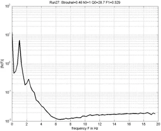
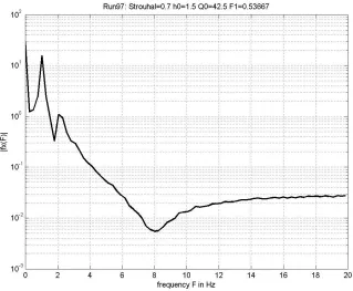
surge force data analysis, a pattern can be identified as shown in Fig.27, Fig.28, Fig.29, Fig.30,

(53)

Figure 27: Surge force spectrum - frequency domain pattern for one type of data

(54)

(55)

(56)

During the data analysis process, each surge force FFT set is observed in order to see

whether there is zero, second order harmonics. However, as can be seen in the analysis above,

zero and second harmonics are the dominant in comparison to other harmonics. Per the

observation of all output surge data series, motion frequency (combined heave and pitch

oscillation) is half of the dominant second order harmonic frequency of the FFT spectrum

analysis for surge forces. Also, the spectrum value which is a complex number can be calculated

with respect to zero order and second order frequency for all data series. Surge force system

seems to be a nonlinear system based on this information. Thus, the response’s Associated

Transform will be used to make data analysis for surge force.

In addition, in order to validate the FFT algorithm developed in MATLAB, comparison

was made between the period of some of surge data in time domain and the frequency of surge

force analyzed by FFT code in MATLAB.

T f  1

(57)

Figure 33: One of surge force in time domain for first data

(58)

The dominant frequency in Fig.34 is 0.22 [1/s] which corresponds to a 4.54 [s] period and

the surge motion period in Fig.33 is close to 4.5 [s]. Using such comparisons, the FFT code can

be validated to work.

In summary, by using the FFT algorithm in MATLAB, surge force data series was

transformed from time domain to frequency domain. Thus, surge force can then be observed

easily and it is possible to observe whether surge force data series is linear or nonlinear system.

As mentioned earlier, most of surge force data outputs have double significant content of

frequency in comparison to the frequency of motion. Therefore, surge force will be analyzed as a

nonlinear system. Next step will be the explanation of the response’s Associated Transform and

how to implement for our surge force data series to obtain data points.

The inputs and the outputs of the flapping fin system have been defined before. It will

now be presented how to implement the response’s Associated Transform for input signals and

output signals. First of all, the nonlinear data analysis method will be explained with Associated

Transform. In addition to this, how the Associated Transform is used to compute data points of

the surge force system.

Here the surge force generation system can be considered as a black box along with

unknown nonlinear properties of flapping fin system. This black box is time invariant which

means that the properties of black box do not depend on time [53]. Signal y(t) is called the

system’s response and A(t) is called the virtual input signal that combines heave and pitch

(59)

Figure 35: Nonlinear surge force system

The Associated Transform is used in order to calculate the data points of the system. The

Fourier Transform values of inputs and outputs have been used for computing transfer functions

of the system.

Before explaining how to obtain each data, it is better to provide some fundamental

information about response computation and the Associated Transform.

Associated Transform is needed in order to calculate data points. The Fourier Transform

of output signal Y(f) will be derived from Yn(f1,…,f2) by reducing all but one variables. Then a

single variable inverse Fourier Transform is necessary to compute y(t). However, in our process,

Fourier Transform is initially implemented for input and output signals. Then, the data points of

the system can be calculated given each point of Fourier Transform coming from CFD analysis.

The process is to calculate Y(f) is called the associated transform [54].

The notation below is used to denote association of variables;

)] ,..., ( [ )

(f A Y f1 f2

Y  n n

In this study, n=2 since second order nonlinear system is considered. Now, the extension

to the general case can be made easily. For the Fourier Transform Ys(f1,f2), the associated

(60)

)] , ( [ )

(f A₂ Y₂ f₁_, f₂

Y 

Inverse Fourier Transform can be then expressed as below;

2 1 2 2 2 1 2 2 2 1 2 2 2 1 1 ) , ( ) 2 ( 1 ) ,

( Y f f e e dfdf

i t

t

y i ft i ft







 



And along with setting t1=t2=t, the equation can be written as it is;

2 2 1 2 2 1

2( , ) 1 ] 2

2 1 [ 2 1 )

( Y f f e df e df

i i t

y i ft i ft

 



     

Now the variable of integration needs to be changed by writing

2 1 f

f f  

2 2 ) ( 2 2 2 2 2 2 _] ) , ( 2 1 [ 2 1 )

( Y f f f e df e df

i i

t

y i  f f t i ft

 



        

All in all, once the order of integration is changed, the equation below is obtained;

df e df f f f Y i i t

y i ft

  2 2 2 2

2( , ) ]

2 1 [ 2 1 ) (



       

It can be seen from the equation above, that term in the bracket should be equal to

)] ( [ )

(f F y t

Y 

(61)

If the integral is rewritten, another formula for the association operation is obtained



     2( 1, 1) 1

2 1 )

( Y f f f df

i f

Y



After providing basic information about the Associated Transform, the theory is

implemented for the CFD data series in MATLAB. First of all, the Fourier Transform is applied

to virtual input signals. This function is defined as “virtual fictitious” signal due to the fact that it

consists of heave motion and pitch motion. This combined input signal is created in order to

calculate the points of transfer functions of the system effectively.

A(t) virtual input signal is defined as below;

) 2 sin( )

(t A Ft

A  

Where; A is defined as virtual amplitude and defined as below;

2 0 2 0 

 h A

Where; h0 is defined as the heave motion amplitude and θ0 as pitch motion amplitude.

After defining the virtual fictitious input signal, the Fourier Transform of the virtual input will be

applied for transform.



 

 A t e dt f

A( ) ( ) i2ft







 Asin(2Ft)e i2ftdt

(62)

2 ) cos( it it e e t  

 &

i e e t it it 2 ) sin(    dt e i e e A f

A i ft

Ft i Ft i    2 2 2 ) 2 ( ) (     



  ] [ 2 2 2 2 2



       _

 e e dt e e dt

i

A i Ft i ft i Ft i ft

By using Dirac’s delta function property, the virtual input signal in Fourier domain can

be obtained as below;



  _ _ ) ( 2 F f dt e i Ft 

)] ( ) ( [ 2 )

( f F f F

i A f

A     

This equation will be used for computing Fourier Transform of the output function with

Associated Transform.

Surge force data points can be calculated based on Associated Transform.

Surge force signals can be expressed before as below;

) ( ) ( ) , ( ) ,

( ₁ ₂ ₁ ₂ ₁ ₂

2 f f H f f A f A f

Y 

Data points can be expressed as below;

(63)

Along with the transfer function points relationship above, surge force can be expressed

as below;



 

 ₂( ₂, ₂) ₂ 2

1 )

( Y f f f df

i f

Y



Data points relationship can be substituted into surge force signal and the new expression

between input and output can be achieved along with Associated Transform.

2 1 f

f f  

2 2 2 2

2, ) ( ) ( )

( 2

1 )

( H f f f A f f A f df

i f

Y





  

 

This equation above shows the relationship between the combined motion of the flapping

fin and the surge force obtained by CFD code.

The input signal which is the motion of flapping fins can be found in Fourier domain to

be; )] ( ) ( [ 2 )

( f F f F

i A f

A     

The input signal can be expressed as below;

)] ( ) ( [ 2 )

( ₁ f₁ F f₁ F i

A f

A     

Along with Associated Transform, the equation can be expressed as below

2 1 f