Variable Neighborhood Search Methods for the Dynamic Minimum Cost Hybrid Berth Allocation Problem

(1)

471

Information Technology and Control 2018/3/47

Variable Neighborhood

Search Methods for

the Dynamic Minimum

Cost Hybrid Berth

Allocation Problem

ITC 3/47

Journal of Information Technology and Control

Vol. 47 / No. 3 / 2018 pp. 471-488

DOI 10.5755/j01.itc.47.3.20420 © Kaunas University of Technology

Variable Neighborhood Search Methods for the Dynamic Minimum Cost Hybrid Berth Allocation Problem

Received 2018/03/24 Accepted after revision 2018/08/16

http://dx.doi.org/10.5755/j01.itc.47.3.20420

Corresponding author: knatasa@ac.me

Nataša Kovač

Faculty of Applied Sciences, University of Donja Gorica, Donja Gorica, 81000 Podgorica, Montenegro, knatasa@ac.me

Tatjana Davidović

Mathematical Institute of the Serbian Academy of Science and Arts, Kneza Mihaila 36, 11000 Belgrade, Serbia tanjad@turing.mi.sanu.ac.rs

Zorica Stanimirović

Faculty of Mathematics, University of Belgrade, Studentski trg. 16/IV, 11 000 Belgrade, Serbia, zoricast@matf.bg.ac.rs

This study considers the Dynamic Minimum Cost Hybrid Berth Allocation Problem (DMCHBAP) with fixed handling times of vessels. The objective function to be minimized consists of three components: the costs of positioning, waiting, and tardiness of completion for all vessels. Having in mind that the speed of finding high-quality solutions is of crucial importance for designing an efficient and reliable decision support system in container terminal, metaheuristic methods represent the natural choice to deal with DMCHBAP. Four vari-ants of Variable Neighborhood Search (VNS) metaheuristic are designed for DMCHBAP. All four proposed VNS methods are evaluated on four classes of randomly generated instances with respect to solution quality and running times. The conducted computational analysis indicates that all four VNS-based methods repre-sent promising solution approaches to DMCHBAP and similar problems in maritime transportation.

(2)

1. Introduction

Berth Allocation Problem (BAP) is one of the most studied topics in the optimization of maritime trans-portation. BAP assumes that a set of vessels needs to be allocated to the berths within some planning hori-zon in such a way that some objective function is opti-mized. BAP is proved to be NP-hard in [32]. The most detailed classification scheme for BAPs is proposed in [2] and extended in [3]. The classification is based on four attributes: spatial, temporal, handling time and performance measure.

Spatial attribute classifies BAPs as discrete, continu-ous, hybrid, or draft. In the discrete case (DBAP), each vessel may be allocated only to one berth at a time, while in the continuous case, a vessel can be allocated to any position on quay. Hybrid layout (HBAP) is ob-tained if vessels can share one berth or one vessel can occupy more than one berth. The fourth BAP layout describes vessel’s berthing position based on its draft. The most common BAP models with respect to the temporal attribute are static and dynamic. In the stat-ic model, arrival times impose soft constraints on the berthing times, meaning that a vessel can be speeded up or slowed down. The dynamic model assumes fixed arrival times of the vessels, meaning that they cannot berth before the expected arrival time. According to the handling time attribute, BAP can assume fixed or variable handling times. Handling times may vary de-pending on the berthing position, on the assignment of Quay Cranes (QCs), or on a QC operation schedule. The performance measure attribute describes the ob-jective function of a considered BAP. Detailed surveys of BAP variants can be found in [3] and [44].

This paper considers a variant of dynamic BAP, de-noted by Dynamic Minimum Cost Hybrid Berth Al-location Problem (DMCHBAP) and classified as

1 2 3

| | | ( ),

hybr dyn fix

∑

w pos w wait w tard+ + according to the notation from [2]. Hybrid layout studied in this paper, corresponds to the case shown in Fig. 3d from [2]. The objective function is based on the one proposed in [40] and it is adapted to the dynamic BAP. The objec-tive function is a weighted sum of three components: berthing of a vessel apart from its preferred berthing position, waiting of a vessel with respect to the expect-ed arrival time, and tardiness of a vessel against its due date. This form of objective function reflects the real requirements in majority of ports [16, 39, 40, 48].

Terminal manager needs a fast and efficient decision support system, in order to meet all requirements of the port as a highly dynamic system. The necessity of quickly providing high-quality solution for BAP was a motivation for many authors to apply metaheuristic methods, such as: simulated annealing, tabu search, ant colony optimization, particle swarm optimiza-tion, etc. [25]. On the other hand, experimental results from [7] related to static MCHBAP, showed that even small BAP instances are too complex for exact and MIP-based heuristics solvers. These results, as well as the fact that dynamic BAP is harder to solve than its static variant [11], motivated us to use metaheuris-tic methods as solution approaches to DMCHBAP. To the best of our knowledge, the only paper dealing with hybrid variant of dynamic BAP is [47]. The au-thors considered hybrid BAP in bulk ports with an aim to minimize the total service times of vessels and applied Squeaky Wheel Optimization (SWO). Hav-ing in mind that the objective function of our DM-CHBAP is different from the one considered in [47], SWO from that paper cannot be directly applied to DMCHBAP. We have developed several variants of SWO adapted to the considered BAP. However, even the best SWO variant provided results that are far from satisfactory ones, with respect to both solution quality and running times (see Section 5). Therefore, SWO is excluded from our consideration as a solution method to DMCHBAP.

(3)

ob-473

served as 2-D packing problems, with the goal to pack smaller rectangles into a bigger one of predetermined size. The main characteristic of this kind of problems is that, in order to improve a given (locally minimal) solution, it is required to significantly degrade its quality by some specific transformations. Although VNS, as an improvement forcing method, may not seem as adequate solution approach, the studies [6] and [26] showed that the use of sophisticated data structures and definitions of neighborhoods in VNS-based methods ensure their good performance when solving static MCHBAP. Therefore, starting from VND [6] and GVNS [26], we have designed VND and GVNS approaches for DMCHBAP. In addition, we develop a Multi-Start VND (MS-VND) and Skewed Variable Neighborhood Search (SVNS) as new VNS-based methods for DMCHBAP. The proposed VNS approaches use adequate solution representation, neighborhood structures, and search strategies, which are adapted to the considered DMCHBAP. All four metaheuristic approaches are evaluated on four classes of randomly generated DMCHBAP test in-stances.

The rest of this paper is organized as follows. A brief review of recent papers addressing metaheuristic ap-proaches to dynamic variants of BAP is given in Sec-tion 2. SecSec-tion 3 introduces the considered DMCH-BAP. In Section 4, we provide a detailed description of four VNS-based metaheuristic for DMCHBAP: VND, MS-VND, GVNS, and SVNS. Experimental results and analysis are presented in Section 5. Concluding remarks and some directions for future work are giv-en in Section 6.

2. Related Work

In recent literature dealing with dynamic BAP, dy-namic vessel arrivals are considered and addressed by several variants of metaheuristic methods, such as randomized Local Search (LS), Tabu Search (TS), Genetic Algorithm (GA), Simulated Annealing (SA), Particle Swarm Optimization (PSO), etc. Nishimu-ra et al. [36] presented GA for the discrete space and dynamic vessels’ arrival times for berth scheduling problem. Imai et al. [21] presented a formulation of the dynamic discrete BAP at a terminal with indented berths, and proposed GA as a solution method. Han et

al. [17] combined GA with SA in the case of dynamic discrete BAP in order to minimize the total service time of all the vessels. Theofanis et al. [45] present-ed an optimization-baspresent-ed GA for the dynamic dis-crete BAP with an aim to minimize the total weighted service time of vessels that may have various service priorities. Dynamic berth allocation and Quay Crane Assignments Problem (QCAP) was considered in [4]. A hybrid method, obtained by combining parallel GA and a constructive heuristic algorithm for generat-ing promisgenerat-ing solutions, is applied to solve QCAP. Discrete space and dynamic vessel arrival BAP with stochastic vessel handling times and known probabil-ity distributions was studied in [22]. Two objectives were considered, risk and total service time, which were minimized by Evolutionary Algorithm (EA). Golias and Haralambides in [14] concurrently min-imized vessels’ tardiness and waiting time and max-imized the premium from vessels’ early departure in the case of dynamic discrete BAP. As a solution meth-od, the authors used GA previously proposed in [15]. Hierarchical optimization approach for dynamic dis-crete BAP was studied in [42], involving two conflict-ing objective functions that correspond to two levels of hierarchy. To solve this problem, the authors de-signed GA based on the k-th best algorithm. The stud-ies [49] and [50] considered dynamic discrete BAP that minimizes total waiting time of calling vessels, where arrival times and handling times of vessels were considered as stochastic parameters following the normal distribution. In both papers, a reduced search space GA, based on the characteristics of the optimal solution, was used. In [41], dynamic contin-uous BAP and QCAP were studied and addressed by GA approach. Two conflicted objectives were consid-ered: minimizing the total service time and maximiz-ing the robustness or buffer times.

(4)

weighted sum of service times. In [23], the cost of the non-optimal berthing location and costs of tardiness were minimized in the case of continuous BAP. In [46], PSO was applied for the first time as solu-tion approach to dynamic discrete BAP. Golias et al. [13] used lambda-optimal based heuristic for dy-namic discrete BAP to guarantee local optimality at a predefined neighborhood. In [28] and [29], Partial Optimization Metaheuristic Under Special Intensi-fication Conditions (POPMUSIC) was used for dy-namic discrete BAP with the aim to minimize the to-tal (weighted) service time of the incoming container vessels. The authors developed two variants of the algorithm by hybridization of the metaheuristic ap-proach with mathematical programming. More pre-cisely, CPLEX solver is used to exactly solve defined sub-problems. Based on promising experimental results, the authors concluded that POPMUSIC has clear advantage over the best approximate approach-es known to date, and that it can be succapproach-essfully ap-plied to this kind of problems as stand-alone solution technique. Hybridization of POPMUSIC and the branch-and-cut algorithm incorporated in CPLEX solver is also used in [30] in the case of BAP under time-dependent limitations where berthing depends on tidal and water depth constraint. A new model for the dynamic BAP was proposed by Simrin and Diabat in [43]. The authors used GA to minimize the total time that vessels spend at a terminal. Alsoufi et al. [1] proposed a mathematical model for robust berth allo-cation and implemented hybrid meta-heuristic based on GA and Branch-and-Cut algorithm in order to minimize the total tardiness of vessel departure time and to reduce the cost of berthing.

Gargari and Niasar in [10] applied VNS method to minimize vessels waiting time and berth idle time in the case of the discrete dynamic BAP. The authors used two types of neighborhoods (insert and swap), which were explored only in the case when a new allocation produced a feasible solution. Discrete dy-namic BAP under tidal and water depth constraints is solved in [27] by applying Adaptive VNS. This variant of VNS involves multi-start strategy that exploits an adaptive mechanism with the goal to minimize the service time of each vessel. In [8], VNS approach was used to solve tactical BAP that incorporates uncer-tainty in vessel arrival times. VNS for tactical BAP is based on two neighborhood structures: reinsertion

movement, which is used in shaking phase and in VND part of local search, and interchange movement, which is explored only in VND part. An overview of solution approaches to different variants of BAP can be found in [25].

3. Dynamic Minimum Cost Hybrid

Berth Allocation Problem

DMCHBAP, considered in this paper, deals with as-signing a berthing position and a berthing time to each incoming vessel to be served within a given planning horizon, with an aim to minimize the total berthing cost. This cost consists of three components: the costs of positioning, waiting, and tardiness of completion for all vessels. The vessels are defined by the following set of data: expected arrival time, processing time, length, due date, preferred berth position, and penalties. As illustrated in Fig. 3, a solution to DMCHBAP can be presented in a space-time-diagram. It is assumed that both coordinates are discrete, i.e., the space is modelled by the berth indices, whereas the time hori-zon is divided into segments, such that berthing time of each vessel is represented by an integer. Each ves-sel is represented by a rectangle with the height equal to the length of a vessel (expressed by the number of berths), while the width corresponds to the required handling time. The berthing position and berthing time of a vessel are given in the lower-left vertex of a rectangle, denoted by the reference point of a vessel (marked by the index of vessel in Fig. 3). A berthing plan is feasible if a) the rectangles do not overlap and

)

b all rectangles can fit in the given space-time-dia-gram (see Fig. 3).

In order to define DMCHBAP, we start from the defi-nition of static MCHBAP given in [24] and adapt it to the dynamic version of BAP. DMCHBAP is charac-terized by the input data, objective function, and a set of constraints defining feasible solutions. The input data of DMCHBAP are listed below:

l : Total number of vessels;

m : Total number of berthing positions;

T : Total number of time units in the planning hori-zon (corresponding to T-1 time segments); vessels: Sequence of data describing all l vessels,

(5)

475

vesselsk : 8-tuple with the following structure

vesselk = (ETA a b d s c c ck, , , , , , , ).k k k k ₁k ₂k ₃k

The elements of a 8-tuple vessel_k represent the follow-ing data for each vessel:

ETAk: The expected time of arrival of vesselk;

ak : Processing time of vesselk, if single crane is

used;

bk: Length of vesselk expressed by the number of

berths;

dk : Required departure time of vesselk;

sk: Least-cost berthing location of the reference point of vessel_k;

c1k : Penalty cost, if vesselk cannot dock at its

pre-ferred berth;

c2k : Penalty cost per unit time, if vesselk cannot

berth at ETA_k;

c3k: Penalty cost per unit time, if vesselk is delayed

beyond the required departure time d_k. A feasible solution of DMCHBAP consists of pairs ( ,B Atk k), k= 1,2, , l where Bk∈{1,2, , } m denotes

the lowest berth index allocated to the vessel_k and {1,2, , 1}

k

At ∈  T- represents the minimum time in-dex of a vessel_k. Pair _{( ,}B At_k _k₎ actually corresponds to

the reference point of vesselk,k= 1,2, , l. A feasible solution of DMCHBAP is subject to the following sets of constraints:

Constraints 1. Each berth can be assigned to only one vessel at time segment t, t= 1, , T-1;

Constraints 2. A berth can be allocated to a vessel only between its arrival and departure times.

The goal of DMCHBAP is to minimize the total pen-alty cost including: the penpen-alty incurred as a result of missing the preferred berthing location of the refer-ence point, the penalty resulted by the actual berthing later than the expected arrival time, and the penalty cost arising from the delay of the departure after the required due time. The last two terms influence the ob-jective function only in case they are positive. Similarly to [40], the objective function can be expressed as:

(

1 2 3

)

=1

( ) ( ) ,

l

k k k k k k k k

k

c σ ₊c At ETA_- +₊c Dt d_- +

∑

(1)

where

(2)

Figure 1

Illustration of BAP solution

occupies more than one berth (each equipped by a crane), the processing time will be reduced.

According to the definition of the objective function given in [40], k is expressed by the given double

sum (2). It can be explained as follows: as the vesselk can occupy several berths and only one is

preferred (which usually means that it contains the required equipment for serving the vessel), all other allocated berths have to be penalized. The lack of a proper equipment on these berths requires the engagement of additional equipment and/or labor. For these reasons, the cost of handling a vessel may increase. Finally, (a b_ )_{denotes that this term has impact on the objective function value only if its} value is positive.

Figure 1 Illustration of BAP solution

Note that DMCHBAP is strongly NP-hard, because it can be observed as a machine scheduling problem [9, 38]. Actually, we prove that even the simpler variant of DMHCBAP is strongly NP-hard.

Theorem 1. DMCHBAP is strongly NP-hard even in the restricted case, in which the preferred berth restrictions are ignored and the objective function represents only total weighted tardiness.

Proof. In order to prove this theorem, we show that the well-known identical machine scheduling problem with release dates and minimization of total weighted tardiness can be polynomially reduced to DMCHBAP. In the standard three field scheduling notation [9], the problem can be classified as

| |

m j j j

P r



w T . In order to follow previously given notations, we rename index j to k. We further assume that vessels represent jobs and berths correspond to the machines. Consequently, vessel’s processing time defined by a bk/ k can be observed as job processing time pk, while expected arrival

time ETAk corresponds to the job release time rk. In addition, job’s due date is actually vessel’s due

date dk and the tardiness is calculated in the standard way, assuming that wk =c3k. To ignore preferred

berthing location and waiting time of vessel, the corresponding penalties c1k and c2k are set to zero.

(6)

, > , ( ) =

0, ,

a b if a b a b

otherwise + 

-- _

 (3)

and Dtk=Atk+ a bk/ k, Dtk∈{1,2, , }T , representing the departure time of the vessel_k. Namely, if only one

crane is used to serve the vessel_k, the required

process-ing time is ak. However, if the vesselk occupies more than one berth (each equipped by a crane), the pro-cessing time will be reduced.

According to the definition of the objective function given in [40], σk is expressed by the given double sum (2). It can be explained as follows: as the vesselk can oc-cupy several berths and only one is preferred (which usually means that it contains the required equip-ment for serving the vessel), all other allocated berths have to be penalized. The lack of a proper equipment on these berths requires the engagement of addition-al equipment and/or labor. For these reasons, the cost of handling a vessel may increase. Finally, (a b_- )+ de-notes that this term has impact on the objective func-tion value only if its value is positive.

Note that DMCHBAP is strongly NP-hard, because it can be observed as a machine scheduling problem [9, 38]. Actually, we prove that even the simpler variant of DMHCBAP is strongly NP-hard.

Theorem 1. DMCHBAP is strongly NP-hard even in the restricted case, in which the preferred berth restric-tions are ignored and the objective function represents only total weighted tardiness.

Proof. In order to prove this theorem, we show that the well-known identical machine scheduling problem with release dates and minimization of total weighted tardiness can be polynomially reduced to DMCHBAP. In the standard three field scheduling notation [9], the problem can be classified as P rm| |j

∑

w Tj j. In order to follow previously given notations, we rename index j to k. We further assume that vessels represent jobs and berths correspond to the machines. Consequent-ly, vessel’s processing time defined by a bk/ k can be observed as job processing time p_k, while expected ar-rival time ETA_k corresponds to the job release time r_k. In addition, job’s due date is actually vessel’s due date

k

d and the tardiness is calculated in the standard way, assuming that wk =c₃k. To ignore preferred berthing

location and waiting time of vessel, the correspond-ing penalties c_1k and c_2k are set to zero. The obtained machine scheduling problem is known to be strongly NP-hard, even for m= 1 (see [38]).

4. VNS-Based Metaheuristics for

DMCHBAP

(7)

477

4.1. Basic Definitions and Solution Representation

All four VNS methods proposed in this study are based on the combinatorial formulation for DMCH-BAP and use the same data structures and initializa-tion (preprocessing) phase as in [6] and [26]. As a part of the initialization, for all vessels and for all possible vessel positions in two dimensional plane, the list of 3-tuples elements (berth, time, penalty cost) is creat-ed. This list is denoted by Ψ and it consists of l indi-vidual ξ lists, each corresponding to one vessel. The ξ lists are sorted in non-decreasing order according to the penalty cost values for each vessel individual-ly. The role of ξ lists is to ensure efficient search of the solution space by its significant reduction in each step. More precisely, any change in the allocation of vessels produces changes in the corresponding ξ lists in such a way that, for each vessel, only feasible posi-tions remain as the elements in its ξ list. The fact that the ξ lists remain sorted at each step of the search, makes it easy to detect positions with smaller pen-alty costs for each allocated vessel (if any exists). In addition, Ψ list structure enables easy identification of unfeasible solution: if at any moment there exists a vessel with empty ξ list, the corresponding solution could be discarded as unfeasible.

During the execution of VNS-based methods for DM-CHBAP, two main decisions are to be made: the se-lection of a vessel to be allocated and the sese-lection of its position in berth-time plane. In the initialization phase of algorithms, these decisions are made sto-chastically, based on the priorities of vessels.

All four VNS approaches proposed for DMCHBAP use the same solution representation based on se-quence pair, which was introduced in [35]. It involves two types of permutations, denoted by H and V that describe the positions of vessels in the port. These permutations are formed based on the following rules:

a if vessel j precedes vessel i in the permutation H, then vessel j “cannot see” vessel i on “left-up” view,

b if vessel j precedes vessel i in the permutation V, then j “cannot see” i on “left-down” view.

For each of the implemented VNS-based methods for DMCHBAP, global variables are: current solu-tion (Solution), local improvement of the shaken current solution (LocalBest), the best found solution

(GlobalBest) and the CPU time of the first occurrence of the best found solution (minT).

4.2. VND for DMCHBAP

Each vessel allocation may be uniquely represented as a pair of permutations ( , )H V . On the other hand, each pair ( , )H V corresponds to a class of allocations. Therefore, the study [6] introduces a procedure that efficiently finds a feasible allocation that minimiz-es total cost while prminimiz-eserving ( , )H V ordering in the case of static MCHBAP.

selection of a vessel to be allocated and the selection of its position in berth-time plane. In the initialization phase of algorithms, these decisions are made stochastically, based on the priorities of vessels.

All four VNS approaches proposed for DMCHBAP use the same solution representation based on sequence pair, which was introduced in [35]. It involves two types of permutations, denoted by H and V that describe the positions of vessels in the port. These permutations are formed based on the following rules:

(a) if vessel j precedes vessel i in the permutation H, then vessel j "cannot see" vessel i on "left-up" view,

(b) if vessel j precedes vessel i in the permutation V, then j "cannot see" i on "left-down" view.

For each of the implemented VNS-based methods for DMCHBAP, global variables are: current solution (Solution), local improvement of the shaken current solution (LocalBest), the best found solution (GlobalBest) and the CPU time of the first occurrence of the best found solution (minT).

4.2 VND for DMCHBAP

Each vessel allocation may be uniquely represented as a pair of permutations ( , )H V . On the other hand, each pair ( , )H V corresponds to a class of allocations. Therefore, the study [6] introduces a procedure that efficiently finds a feasible allocation that minimizes total cost while preserving ( , )H V ordering in the case of static MCHBAP.

The pseudo-code of the VND for DMCHBAP is presented in Alg. 4.2. The procedure used for generating initial solution for VND and GVNS from [6] and [26], respectively, cannot be applied to DMCHBAP, as this procedure often creates infeasible solution. For this reason, we propose two new methods for generating initial solution for DMCHBAP, which are incorporated in the procedure INITIALSOLUTION. Both methods start with creating the subsets of conflicting vessels, based on their most preferred berths and ETA parameter values. In the first method, groups are sorted in non-increasing order of their cardinality. One by one, groups are allocated such that total cost of each group is minimized. If no feasible solution is obtained, the second method is applied. The groups of conflicting vessels are now sorted in

(8)

pro-cedure PermutatIonS. The group of vessels ωS that are not placed on their most preferred positions is identi-fied. The vessels belonging to ωS are sorted in non-in-creasing order of their costs with respect to the current best solution. During the algorithm’s run, the content of set ωS may change, however, its elements are al-ways sorted according to the corresponding costs. As in [6], VND uses three types of neighborhoods, which are applied only to the vessels from ωS. The algorithm always starts from the vessel in ωS hav-ing the largest cost and continues with vessels havhav-ing smaller costs. For a given size k, k= 1,2,3,...kmax, the

neighborhoods are explored in the following order:

1 ChangePoSItIonh: selected vessel is first moved k positions to the left in permutation H, and if there is no improvement, the same vessel is moved k po-sitions to the right in H, while permutation V re-mains unchanged;

2 ChangePoSItIonV: selected vessel is first moved k

positions to the left in permutation V, and if there is no improvement, the same vessel is moved k po-sitions to the right in V, while permutation H re-mains unchanged;

3 ChangePoSItIonhV: represents a combination of

ChangePoSItIonh and ChangePoSItIonV, where all possible changes of H and V are considered. 4.3. MS-VND for DMCHBAP

At the beginning of each iteration of MS-VND, the initial solution is constructed by procedure InItIal-Ize. This procedure starts with an empty solution and constructs a complete initial solution. In order to gen-erate it, the procedure must make two decisions: to choose a vessel and to choose allowable position from

ξ

list for the selected vessel.

corresponding rectangle associated to the vessel in two dimensional plane, and the calculated average cost of all possible ξ list elements for the observed vessel. Coefficients of these three parameters are denoted by λ₁, λ₂, and λ₃, respectively. The linear combination of parameters with the corresponding coefficients represents the priority of a vessel used for its selection by the roulette wheel. The values of coefficients λ_i are determined experimentally in such a way that λ λ λ₁+ ₂+ ₃ = 1 holds.

For a selected vessel, all potential positions are con-sidered with respect to the penalty cost value. The se-lection of vessels’ positions in the initialization phase of MS-VND is performed stochastically, based on the position costs. The positions with smaller costs have higher chances to be selected by the roulette wheel. Procedure InItIalIze calculates probabilities for all feasible positions from ξ list and selects a position by using randomly generated number and the roulette wheel. The considered vessel is fixed on that position and ξ lists are reduced for all unused vessels. The above described process is repeated l times.

From the constructed initial solution, algorithm forms permutation pair ( , )H V and the group of ves-sels ωS. These parameters are further passed as in-put data to algorithm VND1, which is similar to VND described in Subsection 4.2. The only difference is that procedures PermutatIonS and notPreferred -PoSItIon are called outside it and additional input parameters (( , ),H V ωS) are passed to VND1. These steps are repeated until stopping criterion is satisfied (predefined amount of running time RunTime). The best found solution through multiple VND runs is re-turned as the output of MS-VND. The pseudo-code of MS-VND for DMCHBAP is presented in Alg. 4.3. 4.4. GVNS for DMCHBAP

The initial solution and pair ( , )H V are generated in the same way as in VND. GVNS employs Shake pro-cedure based on stochastic transformations of the current best solution. During the shaking step, two transformations are applied in order to form a new solution:

1 First, k random groups of vessels are chosen in

ac-cordance with the priority proportional to the total cost of the group. The chosen groups are placed at the beginning of the list containing all the groups.

non-decreasing order based on average number of feasible positions for vessels belonging to the same group. The allocation of each group is followed by updating the feasible positions in  lists of the remaining vessels and resorting the non-allocated groups.

Based on Solution obtained by procedure INITIALSOLUTION, the corresponding pair ( , )H V is formed by procedure PERMUTATIONS. The group of vessels S that are not placed on their most preferred

positions is identified. The vessels belonging to S are sorted in non-increasing order of their costs with respect to the current best solution. During the algorithm’s run, the content of set S may change, however, its elements are always sorted according to the corresponding costs.

As in [6], VND uses three types of neighborhoods, which are applied only to the vessels from S. The algorithm always starts from the vessel in S having the largest cost and continues with vessels having smaller costs. For a given size k, = 1,2,3,...k kmax, the neighborhoods are explored in the following

order:

(i) CHANGEPOSITIONH: selected vessel is first moved k positions to the left in permutation H, and if there is no improvement, the same vessel is moved k positions to the right in H, while permutation V remains unchanged;

(ii) CHANGEPOSITIONV: selected vessel is first moved k positions to the left in permutation V, and if there is no improvement, the same vessel is moved k positions to the right in V, while permutation H remains unchanged;

(iii) CHANGEPOSITIONHV: represents a combination of CHANGEPOSITIONH and

CHANGEPOSITIONV, where all possible changes of H and V are considered.

4.3 MS-VND for DMCHBAP

At the beginning of each iteration of MS-VND, the initial solution is constructed by procedure

INITIALIZE. This procedure starts with an empty solution and constructs a complete initial solution. In

order to generate it, the procedure must make two decisions: to choose a vessel and to choose allowable position from  list for the selected vessel.

The criterion for vessel selection in MS-VND is a linear combination of ETA parameter, the size of the corresponding rectangle associated to the vessel in two dimensional plane, and the calculated average cost of all possible  list elements for the observed vessel. Coefficients of these three parameters are denoted by 1, 2, and 3, respectively. The linear combination of parameters with the corresponding coefficients represents the priority of a vessel used for its selection by the roulette wheel. The values of

(9)

479

2 Next, k random pairs of vessels are selected based

on the calculated priority, where the priority is proportional to the vessel’s cost in the current best solution. The locations of the selected pairs of ves-sels are swapped. For this transformation, vesves-sels do not need to be in the same group.

Let ( , )H V₁ ₁ be a neighbor solution obtained from Shake phase. Instead of simple local search, GVNS employs VND to find improvements of the solution

1 1

( , )H V , by systematic exploration of its six neigh-borhoods. These neighborhoods are changing H or V permutation, or both permutations simultaneously, with an aim to find the optimal sequence pair. The six procedures for exploring neighborhoods are applied in the following order:

(i) SINGLESWAPH selects two vessels and exchanges their positions in permutation ,H leaving permutation V unmodified;

(ii) SINGLESWAPV selects two vessels and swaps their positions in permutation V, while permutation H is unchanged;

(iii) SINGLEMOVEH selects two vessels vi and vj and moves vessel vj immediately after vessel vi in permutation H, no matter if the vessel vi is in front of or behind vessel

j

v in the current permutation;

(iv) SINGLEMOVEV performs moving of selected vessel v_j immediately after vessel vi in

permutation V, regardless of mutual order of vessels vi and vj;

(v) DOUBLESWAPHV consists of all neighbors obtained by one SINGLESWAPH and one SINGLESWAPV that are not necessarily performed on the same pair of vessels;

(vi) DOUBLEMOVEHV is performed by one SINGLEMOVEH and one SINGLEMOVEV that are not necessarily applied on the same pair of vessels.

GVNS incorporates the first improvement principle. More precisely, when an improvement of the current solution is found in one of the six neighborhoods, the remaining neighborhoods are skipped and this is controlled by noImpr variable. As soon as noImpr gets value false, global variables Solution and GlobalBest are updated inside the corresponding local search procedure. Each procedure of local search starts by examining the value of noImpr variable. The false value will prevent the execution of the corresponding local search procedure. If GlobalBest is improved, the neighborhood counter k is reset to 1. The value of parameter kmax represents the maximal neighborhood size for shaking. GVNS

algorithm finishes when the stopping criterion (predefined amount of running time) is satisfied. The 1 SingleSwapH selects two vessels and exchanges

their positions in permutation H, leaving permu-tation V unmodified;

2 SIngleSwaPV selects two vessels and swaps their

positions in permutation V, while permutation H is unchanged;

3 SInglemoVeh selects two vessels v_i and _v_j and moves vessel v_j immediately after vessel v_i in per-mutation H, no matter if the vessel v_i is in front of or behind vessel v_j in the current permutation;

4 SInglemoVeV performs moving of selected vessel

j

v immediately after vessel v_i in permutation V, regardless of mutual order of vessels v_i and v_j;

5 doubleSwaPhV consists of all neighbors obtained

by one SIngleSwaPh and one SIngleSwaPV that are not necessarily performed on the same pair of ves-sels;

6 doublemoVehV is performed by one SInglemoVeh

and one SInglemoVeV that are not necessarily ap-plied on the same pair of vessels.

GVNS incorporates the first improvement principle. More precisely, when an improvement of the current solution is found in one of the six neighborhoods, the remaining neighborhoods are skipped and this is con-trolled by noImpr variable. As soon as noImpr gets value false, global variables Solution and GlobalBest

are updated inside the corresponding local search procedure. Each procedure of local search starts by examining the value of noImpr variable. The false value will prevent the execution of the corresponding local search procedure. If GlobalBest is improved, the neighborhood counter k is reset to 1. The value of parameter k_max represents the maximal neighbor-hood size for shaking. GVNS algorithm finishes when the stopping criterion (predefined amount of running time) is satisfied. The described steps of GVNS for DMCHBAP are presented in Alg. 4.4.

4.5. SVNS for DMCHBAP

In cases when a high-quality local optimum has been found, VNS will most likely lead the search at random to far-away neighborhoods. As the size of neighbor-hoods to be explored increases, VNS has a tendency to degenerate into a multi-start heuristic. In order to address the problem of getting out of very large neigh-borhoods, Hansen and Mladenović [18] proposed a variant of VNS, denoted by Skewed Variable Neigh-borhood Search (SVNS). The main idea behind SVNS is to accept a local optimum even if it is slightly worse than the incumbent solution. The strategy applied in SVNS helps in solving problem instances having sev-eral separated and possibly distant neighborhoods containing near-optimal solutions [18, 20].

(10)

structure of GVNS described in Section 4.4. As SVNS allows the acceptance of worse solutions compared to the current best one, it was necessary to activate the global variable LocalBest. The initially generat-ed solution is placgenerat-ed in the variable Solution, which is further subject to Shake procedure. Local Search phase tries to improve the newly produced solution by exploring each of the six neighborhoods in the or-der indicated in Alg. 4.5. At the end of Local Search phase, the obtained solution is saved in the LocalBest variable. The difference between GVNS and SVNS is in the acceptance criterion of the local optimum LocalBest produced by VND phase. SVNS is more tolerant in accepting local optimum LocalBest that does not improve the current Solution regard-ing the objective function value. The level of toler-ance is controlled by parameter α> 0.Whenever

( ) | ( ) ( ) |

Cost LocalBest -α Cost LocalBest Cost Solution -is less than Cost Solution( ), the search resumes from

LocalBest by setting k= 1. Obviously, it is necessary to

keep the information about the global best solution GlobalBest and to update it whenever an improve-ment is achieved. As we already explained, this is done within the corresponding local search procedure.

In cases when a high-quality local optimum has been found, VNS will most likely lead the search at random to far-away neighborhoods. As the size of neighborhoods to be explored increases, VNS has a tendency to degenerate into a multi-start heuristic. In order to address the problem of getting out of very large neighborhoods, Hansen and Mladenović [18] proposed a variant of VNS, denoted by Skewed Variable Neighborhood Search (SVNS). The main idea behind SVNS is to accept a local optimum even if it is slightly worse than the incumbent solution. The strategy applied in SVNS helps in solving problem instances having several separated and possibly distant neighborhoods containing near-optimal solutions [18, 20].

This was our motivation to develop SVNS as an additional VNS approach to DMCHBAP. The pseudocode of our SVNS algorithm is presented in Alg. 4.5. The structure of SVNS for DMCHBAP is similar to the structure of GVNS described in Section 4.4. As SVNS allows the acceptance of worse solutions compared to the current best one, it was necessary to activate the global variable LocalBest. The initially generated solution is placed in the variable Solution, which is further subject to SHAKE

procedure. Local Search phase tries to improve the newly produced solution by exploring each of the six neighborhoods in the order indicated in Alg. 4.5. At the end of Local Search phase, the obtained solution

5 Experimental Results

In general, there is a lack of benchmark instances for BAPs in literature. Therefore, we generated test examples randomly, but systematically, following the idea from [12]. Metaheuristics VND, MS-VND, GVNS, and SVNS developed for DMCHBAP are eval-uated on four generated data sets and the obtained results are analyzed. Data sets used in our experimen-tal study are available online at http://www.mi.sanu. ac.rs/tanjad/DMCHBAP.htm. Each of them contains randomly generated instances characterized by the following parameters:

_ the first data set: l= 10,15 vessels, m= 8 berths, the time horizon of T = 15 units, l= 20 vessels,

= 8

m berths, the time horizon of T= 20 units, and = 25

l vessels, m= 8 berths, the time horizon of = 25

T units;

_ the second data set: l= 35,40,45 vessels, m= 8 berths, and the time horizon of T = 112 units;

_ the third data set: contains randomly generated

instances involving l= 50,55,60 vessels in the case of m= 13 berths and T = 112 time units;

_ he fourth data set: l= 70,80,90,100 vessels, m= 13 berths, and the time horizon of T = 112 units. The data used to specify various types of vessels are presented in Table 1 taken from [33]. The set of test instances involves three types of vessels: feeder, me-dium, and mega. For each type, the corresponding percentage of test instances, handling time range, penalty amounts (in units of US$ 1000) and number of berths occupied by specific type of vessels are listed in Table 1. The distribution of the least-cost berthing location for vessels is homogeneous.

Table 1

Vessel specifications for generated test instances

is saved in the LocalBest variable. The difference between GVNS and SVNS is in the acceptance criterion of the local optimum LocalBest produced by VND phase. SVNS is more tolerant in accepting local optimum LocalBest that does not improve the current Solution regarding the objective function value. The level of tolerance is controlled by parameter > 0. Whenever

( ) | ( ) ( ) |

Cost LocalBest  Cost LocalBest Cost Solution is less than Cost Solution( ), the search

resumes from LocalBest by setting k=1. Obviously, it is necessary to keep the information about the global best solution GlobalBest and to update it whenever an improvement is achieved. As we already explained, this is done within the corresponding local search procedure.

5 Experimental Results

In general, there is a lack of benchmark instances for BAPs in literature. Therefore, we generated test examples randomly, but systematically, following the idea from [12]. Metaheuristics VND, MS-VND, GVNS, and SVNS developed for DMCHBAP are evaluated on four generated data sets and the obtained results are analyzed. Data sets used in our experimental study are available online at http://www.mi.sanu.ac.rs/tanjad/DMCHBAP.htm. Each of them contains randomly generated instances characterized by the following parameters:

• the first data set: l= 10,15 vessels, m= 8 berths, the time horizon of T=15 units, = 20

l vessels, m= 8 berths, the time horizon of T= 20 units, and l= 25 vessels, = 8

m berths, the time horizon of T= 25 units;

• the second data set: l= 35,40,45 vessels, m= 8 berths, and the time horizon of T= 112

units;

• the third data set: contains randomly generated instances involving l= 50,55,60 vessels in the case of m=13 berths and T= 112 time units;

• the fourth data set: l= 70,80,90,100 vessels, m=13 berths, and the time horizon of

= 112

T units.

The data used to specify various types of vessels are presented in Table 1 taken from [33]. The set of test instances involves three types of vessels: feeder, medium, and mega. For each type, the corresponding percentage of test instances, handling time range, penalty amounts (in units of US$ 1000) and number of berths occupied by specific type of vessels are listed in Table 1. The distribution of the least-cost berthing location for vessels is homogeneous.

Table 1 Vessel specifications for generated test instances

In order to obtain optimal solutions for small size problem instances we adapted MILP model, proposed in [7] for MCHBAP (the static variant of Minimum Cost Hybrid BAP), to the considered DMCHBAP. We have executed the obtained MILP model within the framework of commercial CPLEX solver, version 12.3, which was run on the same configuration as the one used for metaheuristic methods.

(11)

481

Cost Hybrid BAP), to the considered DMCHBAP. We have executed the obtained MILP model within the framework of commercial CPLEX solver, version 12.3, which was run on the same configuration as the one used for metaheuristic methods.

All four VNS metaheuristic approaches are coded in the Wolfram Mathematica v8.0 programming lan-guage. It is important to note that, unlike classical programming languages, Mathematica interprets in-structions and therefore, the running times of algo-rithms may increase. However, our comparison is fair, having in mind that all VNS-based algorithms are ex-ecuted under the same conditions. All computation-al experiments with CPLEX, VND, MS-VND, GVNS, and SVNS were conducted on the same platform, i.e., on a computer with an Intel Pentium 4 3.00 GHz CPU and 512 MB of RAM, running the Microsoft Windows XP Professional Version 2002 Service Pack 2 operat-ing system. Note that executable version of CPLEX 12.3 is optimized for this platform, meaning that it is favored with respect to other algorithms.

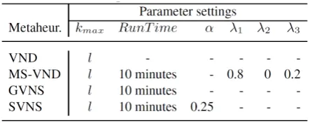
Having in mind that metaheuristics are stochastic methods, their stability is examined by performing repeated runs on each instance. In our computation-al experiments, MS-VND, GVNS, and SVNS methods where executed 10 times with time limit of 10 min-utes for all test examples, i.e., variable RunTime is set to 10 minutes. VND is deterministic in nature, and, therefore, it was run only once on each tested instance. Preliminary computational experiments are per-formed on the subset of test instances in order to de-termine appropriate parameter values for each of the considered VNS-based approaches. Table 2 shows the list of parameter values for each metaheuristic that led to its best performance.

We have also developed several variants of SWO adapted to the DMCHBAP, following the ideas

pre-Table 2

Parameter specifications

All four VNS metaheuristic approaches are coded in the Wolfram Mathematica v8.0 programming language. It is important to note that, unlike classical programming languages, Mathematica interprets instructions and therefore, the running times of algorithms may increase. However, our comparison is fair, having in mind that all VNS-based algorithms are executed under the same conditions. All computational experiments with CPLEX, VND, MS-VND, GVNS, and SVNS were conducted on the same platform, i.e., on a computer with an Intel Pentium 4 3.00-GHz CPU and 512 MB of RAM running the Microsoft Windows XP Professional Version 2002 Service Pack 2 operating system. Note that executable version of CPLEX 12.3 is optimized for this platform, meaning that it is favored with respect to other algorithms.

Having in mind that metaheuristics are stochastic methods, their stability is examined by performing repeated runs on each instance. In our computational experiments, MS-VND, GVNS, and SVNS methods where executed 10 times with time limit of 10 minutes for all test examples, i.e., variable RunTime is set to 10 minutes. VND is deterministic in nature, and, therefore, it was run only once on each tested instance.

Preliminary computational experiments are performed on the subset of test instances in order to determine appropriate parameter values for each of the considered VNS-based approaches. Table 2 shows the list of parameter values for each metaheuristic that led to its best performance.

Table 2 Parameter specifications

We have also developed several variants of SWO adapted to the DMCHBAP, following the ideas presented in [47]. Each of the implemented SWO variants starts from a feasible initial solution and dynamically changes it based on vessels’ priorities. Vessels with larger allocation cost in current solution have higher priority to be chosen for the next allocation. Once feasible solution is produced, all vessels are sorted according to their cost in decreasing order and new allocation starts. One by one, vessels are allocated in port on randomly chosen feasible position by roulette wheel. If allocation leads to an unfeasible solution, a new random solution is generated. In the case that all vessels are allocated in port, i.e., solution is complete and feasible, new vessels’ priorities are calculated and SWO algorithm performs the next iteration. The imposed stopping criterion for each SWO variant is 10 minutes of running time. Implemented SWO approaches for DMCHBAP are also coded in the Wolfram Mathematica v8.0 and executed on the same platform as VNS-based methods. On each instance, SWO was run 10 times. In the rest of this section, we present only the results of the best performing SWO variant.

Tables 3 and 4 contain the comparison of results obtained by CPLEX solver and considered metaheuristic methods on the first data set that includes small size problem instances. The first column of Table 3, denoted by Class contains instance’s specification, given in the form m T l  , where m represents the number of berths, T indicates the number of time units in the planning horizon, and l stands for the number of vessels. The second column contains the identification number (index) of each instance in the corresponding class. The next two columns are related to the results of CPLEX solver, containing objective function value of the optimal solution OPT and the corresponding running time, denoted by

sented in [47]. Each of the implemented SWO vari-ants starts from a feasible initial solution and dynam-ically changes it based on vessels’ priorities. Vessels with larger allocation cost in current solution have higher priority to be chosen for the next allocation. Once feasible solution is produced, all vessels are sorted according to their cost in decreasing order and new allocation starts. One by one, vessels are al-located in port on randomly chosen feasible position by roulette wheel. If allocation leads to an unfeasible solution, a new random solution is generated. In the case that all vessels are allocated in port, i.e., solution is complete and feasible, new vessels’ priorities are calculated and SWO algorithm performs the next iter-ation. The imposed stopping criterion for each SWO variant is 10 minutes of running time. Implemented SWO approaches for DMCHBAP are also coded in the Wolfram Mathematica v8.0 and executed on the same platform as VNS-based methods. On each instance, SWO was run 10 times. In the rest of this section, we present only the results of the best performing SWO variant.

Tables 3 and 4 contain the comparison of results ob-tained by CPLEX solver and considered metaheuris-tic methods on the first data set that includes small size problem instances. The first column of Table 3, denoted by Class contains instance’s specification, given in the form m T l× - , where m represents the number of berths, T indicates the number of time units in the planning horizon, and l stands for the number of vessels. The second column contains the identification number (index) of each instance in the corresponding class. The next two columns are relat-ed to the results of CPLEX solver, containing objec-tive function value of the optimal solution OPT and the corresponding running time, denoted by Time and given in seconds. In the next four columns, results related to the best performing SWO variant are pre-sented. In the column named Best, the best found to-tal cost (obtained after 10 SWO executions) is given, while the average total cost AvgC and average mini-mum CPU time AvgT (out of 10 runs) are presented in the next two columns. In order to measure the quality of the obtained SWO results, in column G%, we pres-ent the average gap calculated as 100 AvgC OPT

OPT

-⋅ .

(12)

running time (in seconds) required by VND to obtain its best solution. The gap G% for VND is calculated as

100 Best OPT OPT

-⋅ . The results of MS-VND, GVNS, and SVNS in Table 3 are given in the same way as in the case of SWO. In order to highlight the best performing method with respect to the solution quality, the best-known (optimal) solutions for each instance are bold-ed in Table 3. Similarly, for the best performing meth-od with respect to CPU time, the shortest (average) CPU times for each instance are bolded in Table 3. From the results presented in Table 3, it can be seen that all four VNS-based methods reach optimal solutions provided by CPLEX solver on each of small size prob-lem instances. SVNS shows the best stability, as its av-erage percentage gap is 0%, meaning that SVNS reached optimal solution in all 10 runs for each instance. The values presented in column G% indicate that MS-VND, and GVNS methods also showed to be stable, as the corresponding average percentage gaps are 0.03%, and 0.09%, respectively. SWO method evinced poor perfor-mance on the set of small size instances, as it provided solutions that are quite far from the optimal ones for each considered instance. The best performing SWO Table 3

Computational results of CPLEX, SWO, and VNS-based metaheuristics on instances from the first data set (m = 8, T= 15, 20,

l = 10, 15, 20)

Table 4

Computational results of CPLEX and VNS-based metaheuristics on instances from the first data set (m = 8, T= 25, l = 25)

Time and given in seconds. In the next four columns, results related to the best performing SWO variant

are presented. In the column named Best, the best found total cost (obtained after 10 SWO executions)

is given, while the average total cost AvgC and average minimum CPU time AvgT (out of 10 runs) are

presented in the next two columns. In order to measure the quality of the obtained SWO results, in column

G%, we present the average gap calculated as 100 AvgC OPT

OPT



 . The next three columns contain results

related to the VND metaheuristic. The column named Best contains the best found total cost. Column

Time indicates the running time (in seconds) required by VND to obtain its best solution. The gap G%

for VND is calculated as 100 Best OPT

OPT



 . The results of MS-VND, GVNS, and SVNS in Table 3 are

given in the same way as in the case of SWO. In order to highlight the best performing method with respect to the solution quality, the best-known (optimal) solutions for each instance are bolded in Table 3. Similarly, for the best performing method with respect to CPU time, the shortest (average) CPU times for each instance are bolded in Table 3.

From the results presented in Table 3, it can be seen that all four VNS-based methods reach optimal solutions provided by CPLEX solver on each of small size problem instances. SVNS shows the best stability, as its average percentage gap is 0%, meaning that SVNS reached optimal solution in all 10 runs

for each instance. The values presented in column G% indicate that MS-VND, and GVNS methods also

showed to be stable, as the corresponding average percentage gaps are 0.03%, and 0.09%, respectively. SWO method evinced poor performance on the set of small size instances, as it provided solutions that are quite far from the optimal ones for each considered instance. The best performing SWO variant produces solutions with average percentage gap of 79.68% from the optimal ones.

Table 3 Computational results of CPLEX, SWO, and VNS-based metaheuristics on instances from the

first data set (m= 8, = 15,20T , = 10,15,20l )

Table 4 Computational results of CPLEX and VNS-based metaheuristics on instances from the first data

set (m= 8, T = 25, l= 25)

Time

and given in seconds. In the next four columns, results related to the best performing SWO variant are presented. In the column named Best, the best found total cost (obtained after 10 SWO executions) is given, while the average total cost AvgC and average minimum CPU time AvgT (out of 10 runs) are presented in the next two columns. In order to measure the quality of the obtained SWO results, in column

G%, we present the average gap calculated as 100 AvgC OPT

OPT 

 . The next three columns contain results

related to the VND metaheuristic. The column named Best contains the best found total cost. Column

Time

indicates the running time (in seconds) required by VND to obtain its best solution. The gap G%

for VND is calculated as 100 Best OPT

OPT 

 . The results of MS-VND, GVNS, and SVNS in Table 3 are

given in the same way as in the case of SWO. In order to highlight the best performing method with respect to the solution quality, the best-known (optimal) solutions for each instance are bolded in Table 3. Similarly, for the best performing method with respect to CPU time, the shortest (average) CPU times for each instance are bolded in Table 3.

From the results presented in Table 3, it can be seen that all four VNS-based methods reach optimal solutions provided by CPLEX solver on each of small size problem instances. SVNS shows the best stability, as its average percentage gap is 0%, meaning that SVNS reached optimal solution in all 10 runs for each instance. The values presented in column G% indicate that MS-VND, and GVNS methods also showed to be stable, as the corresponding average percentage gaps are 0.03%, and 0.09%, respectively. SWO method evinced poor performance on the set of small size instances, as it provided solutions that are quite far from the optimal ones for each considered instance. The best performing SWO variant produces solutions with average percentage gap of 79.68% from the optimal ones.

Table 3 Computational results of CPLEX, SWO, and VNS-based metaheuristics on instances from the

first data set (

m

= 8

, = 15,20T , = 10,15,20l )

Table 4 Computational results of CPLEX and VNS-based metaheuristics on instances from the first data

set (

m

= 8

,

T

= 25

,

l

= 25

)

variant produces solutions with average percentage gap of 79.68% from the optimal ones.

Regarding average running times, GVNS was the fastest in returning its best solutions, followed by VND, SVNS, and MS-VND, while SWO was the slowest method. However, all five methods were significantly faster compared to CPLEX solver, which needed 2436.81 sec-onds (on average) to produce optimal solutions for all instances in the set. The average running times of the proposed VNS-based methods were: 15.74 s for GVNS, 19.58 s for VND, 25.44 s for SVNS, and 77.34 s for MS-VND, while SWO required 241.40 s (on average) to re-turn its best solutions. This implies that the proposed GVNS was more than 154 times faster compared to CPLEX, and 1.24, 1.62, 4.91, and 15.34 times faster than VND, SVNS, MS-VND, and SWO, respectively.

As it can be seen from Table 3, even the best variant of SWO did not produce satisfactory results regarding solution quality and running times. Therefore, SWO is excluded from detailed computational experiments on the other data sets.

(13)

483

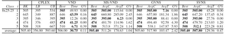
first data set, with m= 8, T= 25, l= 25. For these instances we impose the time limit on CPLEX exe-cution of 1 hour (having in mind that the decisions in the port are to be made very quick, on a minute basis). The first column of Table 4 contains instance’s spec-ification, while the second column, denoted as BK, presents the best-known objective function values, provided either by CPLEX or by the proposed VNS-based metaheuristics. The next two columns are re-lated to the results of CPLEX solver, containing lower and upper bounds on the objective function value of the optimal solution. The rest of Table 4 is related to the results of the four proposed VNS methods, which are given in the same way as in Table 3.

The results presented in Table 4 show that all four VNS-based methods improved upper bounds pro-vided by CPLEX, with the exception of one instance

for which the best solutions of all four VNS methods coincide with the upper bound that CPLEX returned. Again, VND and SVNS showed the best stability, as their average percentage gap is 0.11% and 0.47%, re-spectively. In the case of MS-VND, and GVNS, the val-ues of average percentage gaps were 1.04% and 2.42%, respectively, indicating that these two VNS-based methods also have good stability. On average, VND was the fastest method, followed by GVNS, SVNS, and MS-VND. The average running times of the pro-posed VNS-based methods were: 30.75 s for VND, 103.47 s for GVNS, 129.36 s for SVNS, and 178.63 s for MS-VND, implying that the proposed VND was 3.36, 4.21, and 5.81 times faster than GVNS, SVNS, and MS-VND, respectively.

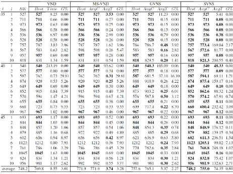
Tables 5 and 6 show the results obtained by the pro-posed VNS-based approaches to DMCHBAP on the

Table 5

(14)

second and third data set, respectively. These data sets contain randomly generated test instances of larger dimensions, unsolved to optimality by CPLEX solver. Therefore, Tables 5 and 6 present the compar-ison of results obtained by VND, MS-VND, GVNS, and SVNS. The first column of Table 5 contains the number of vessels l. The next column (with heading i) indicates the index of the considered instance, while the third column (named BK) refers to the best-known cost value. The results of VND, MS-VND, GVNS, and SVNS are presented in the same way as in Table 3. As optimal solution is not known, the gap G% for VND is calculated as 100⋅Best BK_BK- . In the case of MS-VND, GVNS, and SVNS, the average gap G% is calculated as 100 AvgC BK

BK

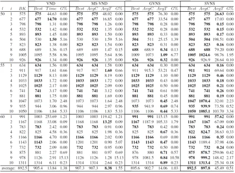
-⋅ . In Table 5, the best-known solutions and the shortest (average) CPU times for the best per-Table 6

Computational results of VNS-based metaheuristics on instances from the third data set (m = 13, T= 112, l = 50, 55, 60)

(15)

485

The results presented in Table 6 on larger size test instances, show that SVNS remains superior to oth-er three methods regarding solution quality. For each test instance from the third data set, SVNS method produced best-known solution at least once with-in 10 runs. On the same data set, SVNS reached the best-known solution in each of 10 runs in the case of 28 out of 30 examples. In the case of instance

= 50

l and i= 10 from the third data set, remaining three algorithms performed better on average with

= 926

AvgC , while for SVNS AvgC= 926.9. For in-stance l= 60 and i= 6 from the same data set, VND and GVNS showed slightly better performance with

=1143

AvgC compared to SVNS with AvgC=1189.4 and MS-VND with AvgC=1201. VND, MS-VND and GVNS have similar performance: GVNS reached best-known solution on 18 out of 30 instances, while VND and MS-VND generated 17 and 16 best-known solutions, respectively. All four methods have small average gaps from the best-known solution: 0.51% for SVNS, 1.03% for GVNS, 1.38% for VND, and 1.55% for MS-VND. MS-VND showed the best performance in respect to CPU time (8.38 s) followed by VND (13.84 s), GVNS (14.06 s) and SVNS (45.49 s). Therefore, MS-VND is 1.65 times faster than VND, 1.68 times faster than GVNS and 5.43 times faster than SVNS. From the presented computational results, it can be seen that the average gap values and required CPU times are quite small for all four VNS based methods, and therefore, all of them can be considered suitable for DMCHBAP. However, SVNS outperforms oth-er methods on both data sets regarding the solution quality, while MS-VND is able to provide high quality solutions in short execution times.

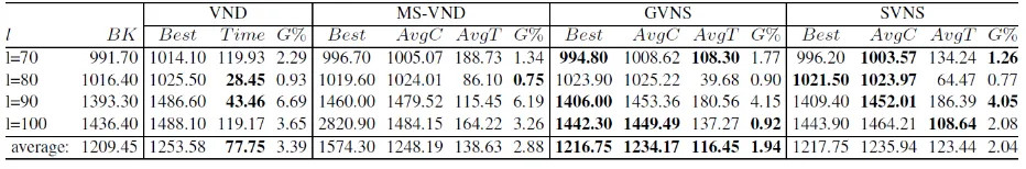
Table 7 shows summarized computational results of the proposed VNS methods on the fourth data set with m= 13, T =112 and l= 70,80,90,100. These test instances are the hardest ones, because of the

Table 7

Computational results of VNS-based metaheuristics on instances from the fourth data set (m = 13, T = 112, l = 70, 80, 90, 100)

large number of vessels and high density of their al-location. Table 7 has the same structure as Tables 5 and 6, the only difference is that each column of Table 7 contains average values obtained on the subset of 10 generated instances (i∈{1,..10}) from the fourth set with fixed value of l. As in the case of the first three data sets, each VNS method is run 10 times on each instance from the fourth data set. On each subclass with fixed value of l, the best result regarding average best cost, average cost, average CPU time and average gap is bolded. The summarized results presented in Table 7 show that all four VNS-based methods have stable performance. On average, the fastest method is VND (77.75 s), however, its average gap is the highest one (3.39%). Other three VNS methods have small computational times with no significant difference among them (between 116.45 s and 138.63 s). On av-erage, VND is 1.50 times faster than GVNS, 1.59 times faster than MS-VND, and 1.78 times faster than SVNS on the fourth data set. GVNS shows the best perfor-mance regarding stability, as its average gap is 1.94%. However, the average gaps of MS-VND and SVNS are also quite small (under 3%). Detailed computational results on these instances can be found at http://www. mi.sanu.ac.rs/tanjad/DMCHBAP.htm.

Computational results presented in Table 7 show that all four presented methods stay stable and efficient even in the case of very hard test instances with large number of allocated vessels. These results verify that VNS based methods can be considered suitable for DMCHBAP and that expected running times on large test instances remain desirable small.

6 Conclusion

In order to meet all requirements of a port as a high-ly dynamic system, terminal manager needs an

As it can be seen from Table 5, SVNS was able to obtain the best-known solutions for all test instances, with average gap of 0.80%. VND, MS-VND and GVNS found best-known solution on 15, 14, and 18 (out of 30) test instances, respectively. However, the resulting average gaps remain very small, 3.01% for VND, 3.28% for MS-VND, and 2.27% for GVNS. Regarding the (average) minimum CPU time, the superior method is MS-VND, followed by GVNS, VND, and SVNS. The corresponding (average) minimum CPU times are 3.74, 5.37, 8.55, and 74.35 seconds, respectively. This means that MS-VND is 1.44 times faster than GVNS, 2.29 times faster than VND, and 19.88 times faster than SVNS.

The results presented in Table 6 on larger size test instances, show that SVNS remains superior to other three methods regarding solution quality. For each test instance from the third data set, SVNS method produced known solution at least once within 10 runs. On the same data set, SVNS reached the best-known solution in each of 10 runs in the case of 28 out of 30 examples. In the case of instance = 50l and = 10i from the third data set, remaining three algorithms performed better on average with

= 926

AvgC

, while for SVNS

AvgC

= 926.9

. For instance = 60l and = 6i from the same data set, VND and GVNS showed slightly better performance with

AvgC

=1143

compared to SVNS with

=1189.4

AvgC

and MS-VND with

AvgC

=1201.

VND, MS-VND and GVNS have similar performance: GVNS reached best-known solution on 18 out of 30 instances, while VND and MS-VND generated 17 and 16 best-known solutions, respectively. All four methods have small average gaps from the best-known solution: 0.51% for SVNS, 1.03% for GVNS, 1.38% for VND, and 1.55% for MS-VND. MS-VND showed the best performance in respect to CPU time (8.38 s) followed by VND (13.84 s), GVNS (14.06 s) and SVNS (45.49 s). Therefore, MS-VND is 1.65 times faster than VND, 1.68 times faster than GVNS and 5.43 times faster than SVNS.

From the presented computational results, it can be seen that the average gap values and required CPU times are quite small for all four VNS based methods, and therefore, all of them can be considered suitable for DMCHBAP. However, SVNS outperforms other methods on both data sets regarding the solution quality, while MS-VND is able to provide high quality solutions in short execution times.

Table 7 Computational results of VNS-based metaheuristics on instances from the fourth data set

( = 13m ,

T

=112

,

l

= 70,80,90,100

)