The use of digital technology to optimize oil pipeline transportation

The use of digital technology to

optimize oil pipeline transportation

by Dr I.K.Beysembetov

1

_{*, T.T.Bekibaev}

1

_{, Dr U.K.Zhapbasbaev}

1

_,

Dr E.S.Makhmotov

2

_{, and Dr B.K.Sayakhov}

2

1 Kazakh British Technical University, Almaty, Kazakhstan

2 JSC KazTransOil, Astana, Kazakhstan

T

HE ARTICLE PRESENTS the results of developing digital technology to optimize ‘hot’ oil pumping. Digital technology is used to model and optimize oil pumping practices in a pipeline section by integrating the SmartTran software and the SCADA system. The problem of selecting optimum pumping practices without heating the oil was solved by D.T.Jefferson who determined the optimum pumping practices in a pipeline section for a fixed oil flow rate, providing that the cost of electricity used by all pumps per unit time was minimal.

The problem of optimizing ‘hot’ pumping has been studied by V.S. Yablonsky. The optimality criterion has been formulated for a fixed oil flow rate. It is not fulfilled when the pipeline throughput and the temperature in a section with several pump stations and heating points is changed.

The algorithm for solving this problem has been constructed with a new approach using the dynamic programming method. The search task is divided into several overlapping subtasks in order to find the optimal substructure. The object of each subtask is the cost function of pumps and preheaters at the stations of the pipeline section. The combination of working pumps and preheaters which gives the minimum cost for energy consumed is being searched for a solution.

The discussion presents the results of ‘hot’ pumping calculations for the Kasymov-Bolshoy Chagan section of the Uzen-Atyrau-Samara trunk oil pipeline. The calculation algorithm was implemented in the SmartTran software for modelling and optimizing ‘hot’ pumping. The initial calculation parameters were loaded from the SCADA system. The SmartTran software calculation results (oil pressure and temperature, pumps power, pumping and heating costs and other parameters) for ‘hot’ pumping are in accordance with the experimental data of the SCADA system.

Energy savings when operating pumps and preheaters can be found provided that the oil temperature in the pipeline section does not fall below the pumping safety conditions. The optimal practice calculation results demonstrate the economic efficiency of ‘hot’ pumping. Thus, the integration of SmartTran software with the SCADA system creates the digital technology for optimizing the technological practices of ‘hot’ oil pumping.

Key words: digital technology, pipeline transportation, optimality criterion, ‘hot’ pumping.

*Corresponding author’s contact details: email: [email protected]

D

IGITAL TECHNOLOGY

processes SCADA system data using software and manages the technological oil pumping process in the pipeline. This technology monitors the operation of pumping units, preheaters, crude oil accepting and of floating tanks,

shut-off valves, etc. All this increases the reliability of the pipeline operation.

to as SmartTran) and the SCADA system of JSC KazTransOil (hereafter SCADA system).

The problem of selecting optimum pumping practices through an oil pipeline without oil heating was first set up and solved by D.T. Jefferson [1, 2]. Jefferson examined an oil pipeline equipped with pumps that have different pressure boosting characteristics. Pressure is regulated at each pumping station. Technological limitations are imposed on the pressure value after the control valve and before the station. These limitations are expressed in the form of the following in equation:

p k p Mi P p p M k n

i k

k k i

i k

min − + ≤ ≤ max − + , = , ,...,

= =

−

∑

∑

0 1

0 1 1

1 2 (1)

where n is the number of pipeline pump stations; p₀ is the net suction head at the source pump station; M_i the pressure loss at the pipeline section between i and i+1 stations;

p_{min k} is the minimum permissible pressure before k+1 station; p_{max k} is the maximum

permissible pressure after k station; P_k is the differential pressure gained by i station.

In this case, the differential pressure P_k at each station can take any value from 0 to the maximum value P_max.

The problem of identifying optimum practices is formulated as follows: at a fixed level of productivity, to find the distribution of differential pressures P_i between the pipeline stations, where the cost of electricity consumed per unit time by all pumping units will be minimal. The technological limitations should be taken into account (1):

F N zi i

n i

= →

=

∑

1

min (2)

where N_i is the power consumed by pumps at i station; z_i is the i station electricity cost.

To solve the optimization problem, Jefferson [2] uses the idea of dynamic programming. For each station with fixed capacity and a given differential pressure, one of the possible combinations to start the pumps must be chosen. In these conditions, the built-up pressure pumps a set output and consumes the least power. This optimization problem has been considered by V.I.Golosovker [3, 4].

In research by L.G.Shchepetkov et al. [5 – 7], a solution is given to the optimization problem for oil pipeline systems using the linear programming method. The algorithms obtained are inferior to the dynamic programming algorithm when solving the problem for a pipeline section with a large number of stations [8].

S.Roberts [9] and J.Hedley [10] have shown the expediency of dynamic programming for solving optimization problems for complex multi-stage processes.

A solution to the problem of optimizing heated oil pumping was first obtained by V.S.Yablonsky et al. [11, 12]. According to V.S.Yablonsky et al. [12], the heating temperature will be optimal when the total cost of pumping and heating per unit length at the beginning of the section is equal to the total cost of pumping and heating per unit length at the end of the pipeline section.

The optimal condition for the fixed oil producing capacity in a pipeline section, as found by V.S.Yablonsky et al. [12], is written as:

ρ

η π ηθθ ρ η π

⋅ ⋅ ⋅Q g iH zH +k ⋅ ⋅D ⋅

(

T −T

)

z = ⋅ ⋅ ⋅Q g i z + ⋅ ⋅k D T⋅ −

H

H H k H

H

k k

1 0 1 ( TT

z

0) θ

θ

where r is the oil density; Q is the volume flow rate; g is the acceleration of gravity; i_H, i_k are the hydraulic slopes in the initial and final pipeline sections; k_H, k_k are the heat-transfer coefficients in the initial and final pipeline sections; z_H, z_θ are the costs of a unit of mechanical and thermal energy; h_H, h_θ are the integral efficiency coefficients of pump stations and station preheaters; T_H, T_k is the initial and final oil temperature in the section; T₀ is the temperature of the surrounding soil; and D₁ is the internal diameter of the pipeline.

In studies [13] on heated oil pumping, the minimum total operating costs for pumping and heating are taken as the optimality criterion, and the target function is written as:

S Q g HzH Q c T T z

H

p H k

= ⋅ ⋅ ⋅ρ + ⋅ ⋅ ⋅

(

−

)

⇒

η ρ ηθθ

min (4)

where S is the total cost for oil pumping and heating in the section; H is the pump pressure, and c_p is the oil’s heat capacity.

Target functions and pumping optimization problems are also considered in studies [14 - 25]. V.S.Yablonsky et al.’s [12] optimal condition is formulated for a fixed oil producing capacity in the pipeline section, and is not fulfilled when the volume pumped is changed, and the oil temperature is regulated in a section with several pump stations and heating points.

The ‘hot’ pumping optimization problem

As is known, 80% of the energy consumed during ‘hot’ pumping is spent on the operation of pumps and preheaters [26]. Therefore, unlike in other studies, the optimization of ‘hot’ pumping is investigated by determining the optimal operating conditions for pumps and preheaters.

The optimality criterion for ‘hot’ oil pumping in a pipeline section with several stations

is determined by the minimum value of the total energy cost used by pumps and preheaters per unit time:

i n

i e j m

ij pmp

ij PU

ij i fuel

j m

ij heat

z i c N z g

pmp

i heat

= = =

∑ ∑

( )

+

∑

1 1 1

l _{k QQ min}

ij fuel

 

 _ → (5)

where m_ipmp _/m

iheat is the number of pumps/preheaters at i station; zeli/zfueli is the electricity cost (tenge/(kWh))/fuel cost (tenge/kg) at i station; cpmp

ij/gfuelij is the integer variable, which has a value of 1 if the pump/preheater is in operation, and 0 otherwise;

NPU

ij is the power consumption of j pumping unit of i station (kWh); kij is the ratio of

rotor rotation frequency to the nominal frequency of the given pump; Qfuel

ij is the rate fuel is supplied to j preheater at i station (kg/h).

The criterion (5) is considered together with pumping safety conditions:

• limitation on pressure at the entrance/exit of the station; • condition for safe preheater operation;

• not allowing oil temperature in the pipeline to drop below the critical temperature (no-flow point).

The preheater’s safety conditions require the following limitations:

Qfuel

The differential in pressure for pumping through a group of pumps is determined by the formula:

∆P Q

c gH Q c c gr op op op , , , , k k ( )=    _      = > 0 0 0

ρ ₍₇₎

where c_op is the number of operating pumps in a group; r is the density of oil being

pumped; H(Q/c_op, k) is the dependence of the pressure on the flow rate of any pump

in the group; k is the ratio of rotor rotations to the nominal frequency of an operating

pump.

Given fixed oil flow, the function of pressure and power consumption generated by a pump or a group of pumps, in addition to the parameter k, will have an independent

variable in the temperature at the pump entrance (denoted by Tpmp

i).

Coefficients of pressure and efficiency characteristics for pumps depend on the toughness of the pumped oil, and the toughness in turn depends on the temperature. Therefore, for the pressure differential and the power consumed, the following dependencies are valid:

∆

P

ijgr

=

∆

P

ijgr

(

k

ij

,�

T

ipmp

)

,�

N

ijPU

=

N

ijPU

(

k

ij

,

T

ipmp

)

The pressure differential satisfies the equation of the balance of pressures [27]:

Pin P T P P P

i n j m ij gr i pmp i n i OHS i PR i sec igr +

( )

=

(

+ + = = =

∑∑

∑

1 1 1

∆ ∆ ∆ ∆

))

+∆Ppb+P

tank (8)

where P_in is the initial pressure; m_igr _{is the number of pump groups at the station; DP}gr ijis the pressure boost generated by the j group of pumps at the i station; DPPR

i is the pressure loss after the pressure regulator; DPsec

i is the loss of pressure in the pipeline, taking into

account the drop in hydrostatic pressure between the i and (i + 1) station where the oil flow is Q; DPpb _{the backpressure value at the final station entrance; P}

tank is the pressure

required to pump oil to the final tank; DPOHS

i are the pressure losses at oil heating

stations.

In the case of ‘hot’ pumping, the pressure losses vary depending on the oil temperature at the station exit. The specified pressure parameters are functions of temperature:

∆Pisec =∆Pisec

(

Ti+∆TiOHS

)

,max_∆Pisec =max_∆Pisec

(

Ti+∆TiOHS

)

where T_i is the oil temperature at the entrance to the i station, DTOHS

i is the heating

value at the oil heating station. The temperature at the exit to the station is equal to (Ti Ti )

OHS

+ ∆ . The temperature at the entrance to the next station can be calculated at a known flow rate, using the value of (Ti Ti )

OHS

+ ∆ _{.This value is equal to the oil}

temperature at the exit of the initial station’s tanks.

The pressure limitations for safe pumping at the entrance and exit before the pressure regulator for the k station satisfy the conditions:`

P_kin P P P P P

in i k j m ij gr i k i OHS i PR i sec i gr = + − + + = − = = −

∑∑

∑

1 1 1 1 1

∆

((

∆ ∆ ∆

)

≥P_kin min ₍₉₎

P_kout P P P P

k in j m kj gr k OHS k out max k gr 1 1 1 = + − ≤ =

When the preheater is located before the pumping station T_k(inpum) =Tk+ ∆TkOHS, the

condition for cavitation-free operation for each l group of pumps at the k station is as follows:

Pklin gr Pkin PkOHS P P

j l

kjgr klminin gr

= − + ≥

= −

∑

∆ ∆

1 1

(11)

For the heated oil flow through each i preheater there is a relationship of the type:

Qi Q P

heat i

heat OHS

=

(

∆ ,gheat

)

(12)

where DPOHS _{is the value of the pressure differential in the bypass pipe;}

gheat ₌

(

_gheat _gheat _{… g}

)

m heat

1 , 2 , , is the vector denoting the operation of each preheater. The

relationship can be determined taking into account the construction of the preheaters at the station.

For each preheater, there is also the relationship of its heating value to the rate of oil flow through the preheater and the rate fuel is supplied to this preheater:

∆Theat ₌C Q Qheat heat fuel ₍₁₃₎

where the constant C_heat depends on the construction of the preheater, its condition, the fuel composition, and the time of year. This value is proportional to the preheater’s efficiency.

There is a specific temperature limit for the oil being pumped. It can be safely heated to this temperature in a preheater so that it does not decompose into separate fractions or evaporate. This value can be denoted as T_oilmax _{In order to take this into account in the} problem model, the following limitation is imposed for each j preheater at the i station:

Ti Tij T C Q Q T

heat

i ij heat

ij heat

ij fuel

oil max

+∆ = + ≤ (14)

Since the heated oil flows with rates Q_iheat_{from each preheater are then mixed with} the unheated bypass flow at flow rate Q Qi

heat

− ∑

(

)

the total heating at the exit of the station at flow rate Q is determined by the formula for mixing flows with different weight coefficients:

∆T g Q ∆

Q T

OHS i m

i heat iheat

i heat

heat

=

=

∑

1

(15)

Using Eqns 12, 13, 15 the relationship of the heating value at the station to the values

DPOHS_,

∅POHS g andQ

i heat

i

fuel_{can be expressed thus:}

∆T ∆

Q g C Q Q P

OHS i m

i heat

i heat

ifuel iheat OHS

heat

=

(

(

)

)

=

∑

1

1

2

,gheat

Each type of oil pumped in the section has a lower limit for cooling temperatureT_oilmin_. Usually its value is linked to the temperature at which oil flow is lost. For this reason it is necessary to impose the limitation:

T x

( )

>Toilmin (16)

where T(x) is the value of oil temperature in a section.

select optimum pumping practices for heated oil, as well as the temperature limitations (6), (14), (16). The main parameters of the problem are the following variables:

cijpmp - the optimum combination of pumps;

gijheat - the optimum combination of preheaters;

Qijfuel - the necessary fuel supply to the preheater;

DPOHS

i - loss of pressure in the heating station.

Solution algorithm

The search task is performed using an approach based on dynamic programming and can be subdivided into a set of overlapping subtasks in order to find the optimal substructure. Using the solution to the problem for n pumps, it is possible to find solutions effectively for n + 1 pumps. A graph of pump operating conditions has been drawn up. Each graph unit contains data on the number of pumps used and their parameters, and the pressure drop in the pressure controller. The units of the graph are connected, based on pump pressure capacity characteristics and rotor rotation frequencies. The transition from the subtask solution to the solution of the general problem has been found and the correctness of this approach has been proved.

The object of each subtask is the function of the relationship of energy consumption cost to the pressure differential generated at the pump.

Naturally, P ≥ 0. The optimum pressure is related to the pumping temperature. In the search for a solution, instead of continuous function S (P,T), its discrete version was used. The pressure value can be represented discretely with a fairly fine pitch

ε_p = 0.01 bar, the temperature value is ε_T = 0.05°C.

The solution of the problem is stored in a discrete array Info (P,T) which for each value P contains a list of the necessary pumps at several previous stations.

The cost function S (P,T) and the solution array Info (P,T) for the pump can be written as:

S P T P P zN Q T P P Info P T P P

pump n

pmp PU

pmp pmp

, ,

, ,

, ,

( )= + ∞ ≠_{( )} = 

 

( )= ∅ ≠

uumber P P, = pmp

  

(17)

where z is the cost of electricity at the station (tenge /(kWh)), N_PU is the pump power (kW), Q is the flow rate passing through the pump.

The pressure differential generated by the pump is found to be:

Ppmp =ρgH Q T

(

,

)



where the operator [ ] denotes rounding up to the nearest rational number in increments of ε_p. The initial cost function is defined as follows:

S P T P P and T T otherwise

in

st. _, , in in ,

1_{( )=}0 =

 

=

+∞ ₍₁₈₎

The ‘combination’ of two functions can be used to denote the function S(P), which for each P has value:

Similarly, the “combination” of two arrays denotes an array Info (P,T) that for each P has the value:

Info P T Info P TA Info P TB Info P T S P T S P T

A A B

, , , , , , � ,

(

)

=

₍

₎

∪

₍

₎

=

(

)

(

)

≤

(

))

(

)

(

)

>

₍

₎

  

Info P T S P TB , � , A , � S P TB ,

The superposition of function SB _{on function S}A_{, denotes function S(P,T), which for}

each P has the value:

S P T

(

_,

)

₌S P TA

(

_,

)

_←

( )

SB ₌min S P T S P P T

(

A

(

_,

)

_, A

(

₋ *_,

)

₊S P TB

(

*_,

)

)

where the value of variable P* for a particular value P is defined as:

P S P P T S P T

P P A B * , * * * , , =

(

(

−

)

+

(

)

)

∈[ ] argmin 0

Likewise, the superposition of array InfoB _{on array Info}A _{is used to denote array Info (P,T)}

which for each P has the value:

Info P T InfoA P T Info P TB Info P T S P T S P P

A A A

, , , , , , ,

*

(

)

=

(

)

←

(

)

=

(

)

(

)

≤ − TT S P T

Info P P T Info P T otherwise

B A B

(

)

+

( )

−

(

)

+

( )

    * * * , , ,

The cost function _S ,

v

heat i _{and the solution array Info} v

heat i,� _{for each i preheater are taken} into account for modes using heating. The independent variables of these are as follows: the first independent variable P indicates the pressure differential at the station; the second independent variable T is the oil temperature at the entrance to the preheater; and the additional third independent variable DT is the increase in the total flow temperature using this preheater.

The preheater cost function has an additional index - the sample size of operating preheaters ν at the station from the set mheat_.

Naturally, ν ≤ 2m heat_{- 1.}

The cost function for operating preheaters and its solution array are calculated as follows:

Sv P T T z Q Q P T Q Q

heat i heat i fuel i v fuel min i fuel ma , , , , ,∆ , ,∆ ,

(

)

=

(

)

∈ xx i

fuel heat

oil max

i v fuel

T T T

Q P T

otherwise , , , , ,   +     ≤ + ∞ ∆ ∆

((

)

=

(

)

( )

(

)

(

)

= ∆ ∆ ∆ ∆

T P T

C Q P v T P T

Q Q heat i heat i heat heat i h ,

,gheat , , eeat

v

heat i ifue

P v T

Info P T T Q

,

, ,

,

gheat

( )

(

)

(

)

=

(

)

+

∆

∆ heater number ll Qi vfuel P T Qmin ifuel Qmax ifuel

heater not worki

, "

, ,

,

(

∆

)

∈  , , 

nng otherwise",

   

(19)

where Q_{i v}fuel

, is the required fuel rate for the i preheater when sampling, DTheat is the heating temperature for the flow through a given preheater.

Vector gheat

( )

v indicates the working combination of preheaters when sampling

ν. Since the superposition operation occurs for values Q_{i v}fuel

, and DTheat when solving

Sv P T T

After calculating all S_vheat i,� _{and Info} v

heat i,� _{, it is necessary to define the cost function S} v OHS and the solution array Info_vOHS _{for the total operation of the preheaters at the station for} each sample ν. Values S_vOHS_{and Info}

v OHS

are defined by the superposition of functions for all operating preheaters:

S P T T S S S

Info P

v OHS

v heat

v heat

v heat g v v

OHS

op

, , ,

, , ,

∆

(

)

= 1← 2 ← … ← ( )

T

T T Infov Info Info

heat

v heat

v heat gopv

,_∆ , , ,

(

)

= 1← 2 ← … ← ( ) ₍₂₀₎

where g_op

( )

ν is the number of operating preheaters when sampling.

The superposition operation for the preheater cost function will take the following form (similar for the solution array):

Sheat A P T T Sheat B min S P T T S P

T

heat A heat B

, _{, ,} , , _{, ,} ,

*

∆ ∆

∆

(

)

←

(

)

=

(

)

+

>0 ,, ,

*

T T∆ −∆T

(

)

(

)

(21)

For any group of three values

(

P T T, ,∆

)

, optimal station operation means the optimal sample of operating preheaters out of mheat _{preheaters. Therefore, the optimal cost}

function for the station is the combination of all possible cost functions from the samples (2m heat_{-1) (similar for the solution array):}

S

OHS

P T T

S

P T T

v v OHS

mheat

, ,

∆

, ,

∆

(

)

=

(

)

= −

1 2 1



(22)

When none of the preheaters at the station operate, the calculated cost function and the solution array should be adjusted:

SOHS

(

_{0, ,}T ₀

)

_=0,InfoOHS

(

_{0, ,}T ₀

)

_="heaters not working_"

Since, unlike the group of pumps, when the oil passes through the station the flow temperature increases and the pressure decreases, the superposition of the heating cost function SOHS _{onto the cost functions of the entire station takes the following form} (similar for the solution array):

S P T

S P T

S

S P P T

T

S

P T

st OHS

P T

st OHS

,

,

,

,

*_, *

* * *

(

)

=

(

)

←

( )

=

(

+

−

)

+

≥

min

∆ 0

(

∆

(

−−

∆

T

∆

T

)

)

*

_,

*

If the preheaters are located after the pumps, then the cost function at the station entrance and its solution array must first be superimposed with the cost functionSOHS and only then with the cost functions of the pump group. Otherwise, the opposite should be done. If there are no preheaters at a station, there is no need to calculate function SOHS _{for it or to superimpose it on the cost function of the station.}

The pressure differential and temperature drop at the section depend on the initial temperature. To properly trim the cost functions and solution arrays at the exit of the station and define the cost functions and solution array at the entrance of the next station, the discrete functions ∆Pisec

( )

T ,∆Tisec

( )

T and max _∆Pisec

( )

T , max _∆Tisec

( )

T should be calculated for each i section in increments of ε_T.

Moreover, the function max _∆Tisec

( )

T determines the maximum value of the

k=1

It is thus possible to define functions P_outmin i T P T

out max i

,

( )

_, ,

( )

_{for the minimum and} maximum allowable pressure at the exit of the station:

P P max P P P

P P

i out

out min i

k in

k sec

i sec i

out o

2

1

2

≥ =

(

+

)

≤

+

, min _{∆ ,max_∆}

uut max i

k out max

k pipe max

min P P

, ₌

(

2 _,

)

In this case, the condition (16) for minimum required temperature at the exit of the station will take the following form:

T_outmin i T Tmin T T

i

,

( )

_{= + _}

( )

oil

sec

max ∆

Cost function trimming at the exit of the station is found from P_outmin T P T T T

out max

out min

( )

,

( )

,

( )

and is denoted as a function which for each P and T has value:

S P T CUT S P T P P T

P P

st

outmin outmax outmin

cut.st _{, , , ,}

, [

,

(

)

=

(

(

)

)

=

+∞ ∉ _ooutmin out

max outmin st

T P T

T T T

S P T

( ), ( )]

,

, ,

+∞ <

( )

(

)

 

otherwise

  

The solution array is trimmed in the same way.

The pressure differential in the preheater will be added to the cost function and the solution array at the station exit. The changed pressure conditions (9) and (10) are automatically taken into account when it is trimmed.

The cost function at the entrance to the subsequent station is determined by the “shift” operation using the cost function at the station exit through ∆Psec

( )

T _{and ∆T}sec

( )

_{T .} This function for each P and T has a value:

S P T SHIFT S P T P T

S

in next st

outst sec sec

T out

st

. _{, , , ,}

min_*

(

)

=

(

(

)

)

=

∆ ∆

PP+ Psec

( )

T T+ Tsec

( )

T

(

)

(

∆ * _, ∆ *

)

The shift operation is performed in the same way for the solution array.

All operations for finding the optimum practices of the ‘hot’ pumping method are thus defined above.

These operations are carried out for all stations except the last one in order of their location in the pipeline section:

1. For i₌₁to mgr k, _calculateS

igr k,

2. If

m

heat,k

>

0

, then it is necessary to calculate SkOHS (19) – (22)

3. _Soutst k _{P T S P T S S S}

inst k kOHS gr k _mgr kk

,

(

_,

)

₌ ,

(

_,

)

_←

( )

_←

( )

, _{← … ←}

( )

, 1

or

Soutst k,

(

P T,

)

=Sinst k,

(

P T,

)

←

( )

S1gr k, ← … ←

( )

S_mgr k,k ←

( )

SOHSk

4. Calculation of functions∆P_ksec

( )

T ,∆T_ksec

( )

T ,max_∆P_ksec

( )

T ,max_∆T_ksec

( )

T

5. _Soutst k _{P T CUT S P T P P T}

outst k outmin k outmax k outmin

,

(

_,

)

₌

(

,

(

_,

)

_, , _, , _, ,,k

)

6. S_inst k,+1

( )

P =SHIFT S

(

_outst k,

(

P T,

)

,_∆P_ksec,_∆T_ksec

)

7. k = k+1. Ifk n≠ +1, then go to step 1, otherwise exit the cycle

After the abocve cycle with initial condition (18) is carried out, the optimal final pressure and temperature are calculated as:

Popt Topt S P T

T T P P in

st n

tank

, ,

,

.

(

)

=

(

(

)

)

≥ ≥

+

argmin

final

1

The minimum cost per unit is the value of function S_inst n.+1

(

Popt,Topt

)

. The optimum combination of operating pumps and preheaters, as well as their operating practices and the required pressure differentials at the station, will be stored in the cell of the array.

Discussion of calculation results

Determining optimum oil pumping practices is important for reducing the power consumption of pumps and preheaters in the Uzen-Atyrau-Samara oil pipeline [25]. Taking into account the extent of electricity and heat consumption for ‘hot’ pumping, even a minor percentage reduction in costs can lead to significant energy savings [14], [23], [25].

Optimum ‘hot’ pumping practices are being sought at the Kasymov - Bolshoy Chagan section of this pipeline. Pumping occurs using the Kasymova and Inder station pumps, while oil heating takes place in the Sakharnii heating station as well as at these stations.

Based on criterion (5) and algorithm (23), SmartTran software was developed to model and optimize ‘hot’ pumping. SmartTran software was integrated with the SCADA fibre-optic system, i.e. parameters for ‘hot’ pumping practices were found by the SCADA system and represent the initial data for SmartTran calculations.

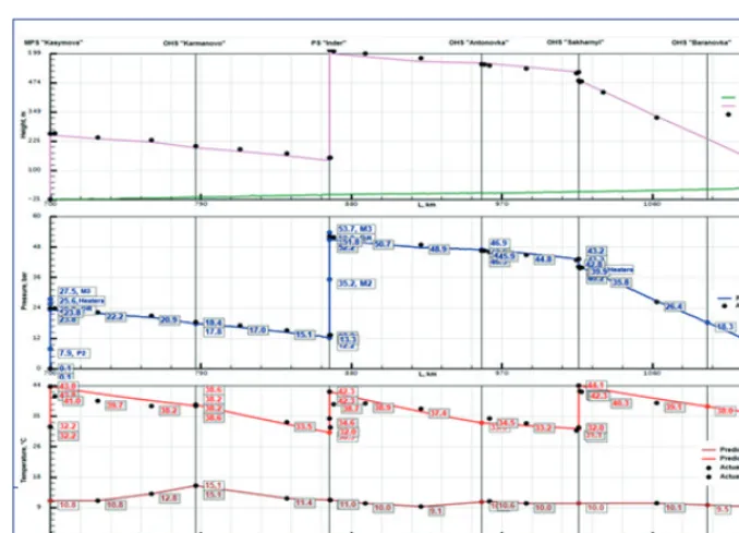
Figure 1 shows the distribution of pressure, the temperature of ‘hot’ pumping at the Kasymov-Bolshoy Chagan section, the operating pump parameters, and the oil heating temperature. The upper part of the figure shows the hydro-slope change. The middle part shows the distribution of pressure, while the lower part shows the distribution of oil and ground temperature. Operating pumps M2 and P2 at Kasymova station, and M2 and M3 at Inder station are marked in Fig.1. Oil is heated at Kasymova, Inder, and Sakharnii stations. The distributions of the hydro-slope, pressure and temperature of the oil blend in Fig.1 were obtained from SmartTran calculations. The points are the experimental data from the SCADA system. The concurrence of calculated data from SmartTran and the SCADA system should be noted.

The upper table (Fig.1) presents oil flow of 1782 t/h, power consumption of 5095 kW, specific electricity consumption of the pumps of 2.86 kWt/h, operating costs of the pumps of 87,000 tenge/h and of the preheater of 1,514,000 tenge/h, specific costs for pumping of 48.8 tenge/t and for heating of 85 tenge/t.

The lower table (Fig.1) shows the values calculated by SmartTran (oil pressure and temperature, pump power), which correspond to experimental data from the SCADA system with accuracy of 1 to 2%.

diameter. Moreover, the average oil flow rate increases 2.04 times.

Figure 2 shows the results of SmartTran calculations and the experimental data of the SCADA system when the drag-reducing agent is added at Sakharnii with a concentration of 3 ppm.

The increase in oil flow to 1918.2 t/h leads to an increase in power consumption to 5,297 kW, in the cost of operating pumps to 905, 000 tenge/h and the preheater to 2,192,000 tenge/h. However, the specific electricity consumption and pumping costs are reduced to 2.76 kWh/t and 47.2 tenge/t, respectively.

This can be explained by the influence of the drag reducing agent, which reduces the hydraulic resistance of the turbulent oil flow.

The specific costs of the preheater increase because a greater quantity of oil is heated. The correspondence between the calculated values for pump power, oil flow parameters and the experimental data from the SCADA system can also be noted here (Fig.2).

When ‘hot’ pumping, the main costs relate to heating oil. Optimization calculations were therefore carried out to determine

an effective heating temperature for oil.

Figures 3 and 4 show the calculated data obtained for the same oil flow rate of 1779.2 t/h and ground temperature value.

The results of calculated data in Fig.3 were obtained from the experimental data of SCADA heating temperature at the Kasymova, Inder, and Sakharnii sections.

The results of calculated data in Fig.4 were obtained when the oil heating temperatures at Kasymova, Inder, and Sakharnii were found for optimal operating conditions for the pumps and the preheater. The optimal conditions were determined on the basis of criterion (5), satisfying the conditions for pressure (9) - (11), and oil preheating temperature (6), (14), (16).

In this case, the preheating temperature is adapted at Kasymova, Inder, and Sakharnii, so that the oil temperature at the Kasymov-Bolshoy Chagan section does not drop below 28o_{C. As can be seen}

from Fig.4, the heating temperatures are equal to 42.2°C at Kasymova, 37.7 °C at Inder, and 38.0 °C at Sakharnii.

By contrast, according to SCADA experimental data the heating temperatures equalled 46.3°C at

Fig.1. Calculated data for ‘hot’ pumping

at the flow rate of

Kasymova, 42.1°C at Inder, and 44.1°C at Sakharnii (Fig.3).

It can be noted that given optimum practices, the heating temperatures decrease by 4.1°C at Kasymova, by 5.4 °C at Inder, and by 6.1°C at Sakharnii.

The total capacity of the pumps is 5091 kW (Fig.3) and 5088 kW (Fig.4).

Given optimum practices, the total costs for oil pumping and heating reduce from 2,201,000 tenge/h to 1,621,000 tenge/h, and unit costs from 123.7 tenge/t to 91.1 tenge/t.

Thus, the developed digital technology, by integrating SmartTran software with the SCADA system, makes it possible to determine the energy efficiency of ‘hot’ oil pumping.

Conclusions

Based on the results of these studies, the following conclusions can be drawn:

1. Optimizing ‘hot’ pumping practices includes identifying operating conditions for pumps and oil preheaters where the total

Fig.2. Calculated data for ‘hot’ pumping at a

flow rate of 1918.2 t/h

according to SCADA system data at the Kasymov-Bolshoy Chagan section.

Fig.3. Calculated data for ‘hot’ pumping at a

flow rate of 1779.2 t/h

energy cost value for pumps and fuel per unit time is minimal, and conditions for safe pumping are fulfilled. The expediency of minimizing the total cost, rather than the amount of energy consumed by pumps and preheaters, is explained by the fact that electricity and thermal energy have completely different costs. Therefore, it is reasonable to compare only expenditures from operating pumps and preheaters.

2. The solution algorithm is performed using the new approach of dynamic programming. The search problem is divided into a set of overlapping subtasks in order to find the optimal substructure. The object of each subtask is the cost function of pumps and preheaters at the stations of the pipeline section.

The combination of working pumps and preheaters which provides the minimum total expenditure is being searched for a solution.

Calculated results from SmartTran software (oil pressure and temperature, pump power), for ‘hot’ oil pumping at the Kasymov - Bolshoy Chagan section

correspond to the experimental data of the SCADA system.

The optimal conditions were obtained on the basis of criterion (5), satisfying the conditions for pressure (9) - (11) and oil preheating temperature (6), (14), (16). Energy efficiency of pumps and preheaters was found provided that the oil temperature at the Kasymov-Bolshoy Chagan section did not drop below 28°C. It has been shown that the specific costs for pumping and heating were reduced from 123.7 tenge/t to 91.1 tenge/t. This constitutes a saving of 26.3%.

References

1. J.T.Jefferson, 1960. Dynamic mathematical programming for power cost optimization. IBM Liquid Pipe Lines Computer Workshop, Chicago, November 29. 2. J.T. Jefferson, 1961. Oil and Gas Journal 8

pp 102-107.

3. V.I. Golosevker, 1967. Determination of the trunk oil pipeline operating practices at the given capacity. Transportation Storage of Oil and Oil Products 10 pp 7-9. 4. V.I. Golosevker, 1969. Determination

of economic efficiency of pipeline production gain measures. Transportation Storage of Oil and Oil Products 11 pp 24-26.

5. M. V. Meerov, V.G. Fridman, and L.G. Shchepetkov, 1971. Optimum oil pipeline

Fig.4. Calculated data for ‘hot’ pumping energy-saving practices

at a flow of 1779.2

management problem. M. GRSU OG (Gubkin Russian State University of Oil and Gas) 37 pp.

6. L.G. Shchepetkov, 1971. Multi-line oil pumping pipeline plan optimization. Transportation Storage of Oil and Oil Products 3 pp 15-18.

7. E.V. Vyazunov, L.G. Shchepetkov, and V.I. Golosevker, 1974. Optimum oil pipeline management and assessment of its efficiency Oil Industry 5 pp 17-19. 8. A.P. Tumansky, 2008. Optimization of

hydrocarbon fluid transportation practices through pipelines with relay pumping stations equipped with VFD (variable frequency drive): PhD Dissertation in Technical Science: 25.00.19/ Tumansky Alexandr Petrovich 137 pp.

9. S. Roberts, 1065. Dynamic Programming in the chemical engineering processes and the methods of management. – M. Mir. 480 pp.

10. J. Hedley, 1967. Non-linear and dynamic programming. M. Mir, 506 pp.

11. V. S. Yablonsky and V.D. Belousov, 1959. Oil and gas pipeline engineering design. M: Gostoptekhizdat, 292 pp.

12. S. Yablonsky et al., 1965. Engineering design, operation and repair of oil product pipelines V– M.: Nedra, 410 pp.

13. V. M. Agapkin, B. L. Krivoshein, and V. A. Yufin, 1981. Thermal and hydraulic calculations of pipelines for oil and oil products. M.: Nedra 256 pp.

14. L. S. Abramzon, 1981. Optimum parameters for operation of hot oil pipeline. Oil Industry. M.: Nedra, 256 pp. 15. A. N. Philatova, 2004. Hot Pumping

optimization based on two unrelated characteristics: Materials of Second International Scientific and Technical Conference Novoselovsky / A.N. Filatova, N.A. Harris, Ufa, Issue 2 pp. 184-188. 16. A. F. Yukin, 2004. Thermal practices

transportation management of viscous and congealing oils and oil products: PhD Dissertation in Technical Science: 25.00.19 / Yukin Arkady Fedorovich Ufa 324 pp.

17. R.Kalab, 1960. Some mathematical aspects of optimization problems in engineering. Proc. Symp. Optimization Tech in Chem. Eng. AIChE, Operations Research Soc, NY, May 18 pp 1-26.

18. A. P. Tumansky, 2005. Optimization of hydrocarbon fluid transportation practices through pipelines with relay pumping stations equipped with VFD

(variable frequency drive). Transportation and Storage of Oil and Oil Products 8 pp 11-14.

19. R. R. Gafarov, O.E. Danilin, 2008. Two-level system for optimizing the operation of oil pumping stations in the trunk oil pipeline section. Oil and Gas Engineering 2 pp 105-112.

20. V. A. Shabanov, O. V. Bondarenko, 2012. Target functions and criteria for oil pumping optimization through oil pipelines under VFD (variable frequency drive) of main line pumps. Oil and Gas Engineering 4 pp 10-17.

21. V. V. Pshenin, V. I. Klimko, 2013. Determination of the optimal heating temperature for ‘hot’ pumping of oil and oil products // Mining Informational and Analytical Bulletin (scientific and technical journal) GIAB (Gorny Informatsionno-Analiticheskiy Byulleten (nauchno-teknicheskii zhurnal)) 8 pp 338-342.

22. N. A. Harris, A. N. Filatova, 2000. Determining optimum operating practices for underutilized non-isothermal pipelines. Problems Efficient Use of Resources in the National Economy: Edited Volume. Issue. 1: The Bashkir Encyclopedia.pp. 156-158.

23. R. N. Bakhtizin, A. A. Shutov, K. Y. Shtukaturov, 2003. Optimum choice of technologies for the operation of non-isothermal pipeline. Bashkirsky Chemical Journal. 1 (10) pp 18-20.

24. E. S. Makhmotov, S. A. Rziev, I. K. Beysembetov, U. K. Zhapbasbaev, T. T. Bekibaev, G. I. Ramasanova, 2015. Optimization of practices for restarting the main oil pipeline sections after a short-term stop. Oil Industry 7 pp132-135. 25. U.K. Zhapbasbaev, E. S. Makhmotov, G. I.

Ramasanova, T. T. Bekibaev, S. A. Rziev, 2015. Optimum pumping temperature calculation for oil transportation. Science and Technologies: Oil and Oil Products Pipeline Transportation 4 (20) pp 61-66. 26. V. I. Klimko, 2002. Rationale for the

thermal regime of pipeline transportation of high-viscosity and high pour point oil: PhD Dissertation in Technical Science: 25.00.19 / Klimko Vasily Ivanovich St Petersburg 137 pp.